High dimensional gaussian classification

arXiv: math.ST/ 0806.072 9 High dimension al gaussian classificatio n Robin Girard ?? LJK, Gr eno ble, F r anc e Abstract: High dimensional data analysis is kno wn to b e as a challenging problem (see [ 10 ]). In this ar ticle, we give a theoretical analysis of high dimensional classification of Gau ssian data which relies on a geometrical analysis of the error measure. It links a problem of classification with a problem of nonparametric regression. W e give an algorithm designed for high dimensional data whic h app ears straightforw ard in the light of o ur the- oretical w ork, toge ther with the thresholding estimation theory . W e finally attempt to give a general treatmen t of the problem that can b e extended to frameworks other than gaussian. AMS 2000 sub ject cla ssifications: Primary 62C20. Keywords and phra ses: Classification, High dimension, Gaussian mea- sure, thresholding estimator, dimension reduction, Linear Discriminant Anal- ysis, Quadratic Discr i minant Analysis. Con te nts 1 Int ro duction . . . . . . . . . . . . . . . . . . . . . . . . . . . . . . . . . 1 2 Affine per turbation of affine rules . . . . . . . . . . . . . . . . . . . . . 5 3 Quadratic p erturbatio n of quadra tic rule . . . . . . . . . . . . . . . . . 14 4 Classification pro cedur e in high dimension: a wa y to solve Problem 2 . 19 5 Application to medical data and the TIMIT database . . . . . . . . . 24 6 A more geometric alternative measure of erro r: the lear ning erro r . . . 27 7 A geometrical Analysis of LDA to solve Pro blem 1 . . . . . . . . . . . 3 3 8 A general scheme to solve Problem 1 . . . . . . . . . . . . . . . . . . . 44 Ac knowledgemen ts . . . . . . . . . . . . . . . . . . . . . . . . . . . . . . . 54 References . . . . . . . . . . . . . . . . . . . . . . . . . . . . . . . . . . . . 54 1. Introduction Let X b e a vector spa ce, typically X = R p but X can also b e an infinite di- mensional p olish s pa ce (i.e: s e parable complete metric space). In Section 8 X is a separable Bana ch space. In the binary classifica tion pro blem, the aim is to recov er the unknown cla s s y ∈ { 0 , 1 } as so ciated with a n observ atio n x ∈ X . In other words, we seek a classific a tion rule (also ca lled clas sifier), i.e a mea surable g : X → { 0 , 1 } . This rule giv es an incor rect cla ssification for the observ ation x if g ( x ) 6 = y . The underlying pr obabilistic mo del, that makes a perfo rmance measure of g p os s ible, is set by distributions P k ( k = 0 , 1) on X . F or k = 0 , 1 , the distr ibution P k is the distribution of the data having la be l equal to k . In this 1 imsart-g eneric ver. 2007/12/10 file: article-fina l1.tex date: Octobe r 24, 2018 R. Gir ar d/High dimensional gaussian classific ation 2 framework, the weight ed sum of the pr obabilities of miscla ssification is de fined by C ( π, g ) = π P 1 ( g ( X ) 6 = 1 ) + (1 − π ) P 0 ( g ( X ) 6 = 0 ) . (1) In a bay esian framework, the weigh t π reflects the margina l distribution of the lab el Y . In our approa ch, we do no t wan t this ma r ginal distribution to set the imp ortance of the differen t erro r s. In the man y applications we hav e in mind, such as tumour detection from a n MRI signal, the class that app ear s mos t fr e- quently is not nec e s sarily the one fo r which a class ification er ror has the most impo rtant medical conse q uences. This is the reaso n why we search a pro cedur e g that minimise C ( π , g ) a nd not its bay esia n counterpart : P ( g ( X ) = Y ). Here, we do not wan t to study the influence of the weigh t π in the problem. The main r eason is that our results, to b e g iven later, are simpler to formulate and to understand whe n π = 1 / 2, a nd that the problem we are in terested in is the pr o blem tha t rise from the hig h dimensio n o f the spac e X , and not the prob- lem related to the use of π . T he r efore, in the rest o f the pr esent pa p er we will make the ass umption that π = 1 / 2 . In the sequel, we will set C ( g ) = C (1 / 2 , g ). This is a us ual a ssumption (se e for example Bick el and Levina [ 6 ]) In the case where π = 1 / 2 it is known that, if P 0 and P 1 are equiv alent, then the rule that minimises C ( g ) is given by g ∗ ( x ) = 1 V , V = { x ∈ X : L 10 ( x ) ≥ 0 } where L 10 = log  dP 1 dP 0  (2) is the loga rithm of the likekihoo d ra tio b et ween P 1 and P 0 (i.e the Rado n- Nikodym der iv ative). In rea l life problems, L 10 is unknown, a nd the only thing we hav e is a sub- stitute b L 10 of it. Also, it is natural to plug it in ( 2 ) and to use the class ifie r g ( x ) = 1 ˆ V ( x ) and ˆ V = n x ∈ X : b L 10 ≥ 0 o . The natur al q uestion tha t we will investigate in this article is the following: Problem 1. Is ther e a simple way to r elate the exc ess risk C ( g ) − C ( g ∗ ) to a me asur e of the lo g-likeliho o d ”p erturb ation”: b L 10 − L 10 . In other words we seek an upper b ound and a lower bo und o f C ( g ) − C ( g ∗ ) by a simple-to - study re a l v alue d function o f b L 10 − L 10 . In this ar ticle we fo cus on the gaussian case, and unless the contrary is explicitly s tated, P 1 and P 0 will be ga us sian equiv alent pro babilities on X . W e inv estiga te Pro blem 1 and the answer we o btain in the g eneral ca se leads to the b ound C ( g ) − C ( g ∗ ) ≤ c ( r ) k b L 10 − L 10 k 1 / 6 L 2 ( γ ) while k L 10 k L 2 ( γ ) ≥ r > 0 for a gaussia n measure γ , where c ( r ) is a co nstant o nly depe nding on r . In so me pa rticular cases (when b L 10 − L 10 and L 10 are affine) imsart-g eneric ver. 2007/12/10 file: article-fina l1.tex date: Octobe r 24, 2018 R. Gir ar d/High dimensional gaussian classific ation 3 we are able to give a n explicit constant c ( L 10 ) and a n exp onent higher than 1 / 6 (exp o nent 1 ). If we supp ose that P 0 and P 1 hav e equal cov aria nce, then it is known that L 10 is a ffine and it is natura l to take an affine b L 10 . The co rresp onding pro cedure is usually calle d Linear Discriminant Analysis (LDA) (even if the underlying pro- cedure is a ffine). If we s uppo se that P 0 and P 1 hav e different cov ariance, then L 10 is quadratic and it is natural to take a quadra tic b L 10 . The co rresp onding classification pro cedure will be calle d Quadr atic Discriminant Analys is (QDA). The corresp o nding pro ce dures are also k nown as plug-in pro cedures: b L 10 is plugged into ( 2 ) in order to o btain g . Plug- in pro cedur e hav e b een studied in a differ e n t context (see for exa mple [ 3 ] and the r eferences therein), but our ap- proach differs fr o m those . The interest o f Pro ble m 1 in the g aussian setting, is understo o d by a ddressing the problem of finding a go o d substitute b L 10 for L 10 . F or example, in man y applications, we are given a learning set consis ting of n rando m v ariables drawn independently fr om P 1 and n ′ drawn from P 0 . The problem of finding a g o od substitute b L 10 of L 10 then b eco mes an estimation pro blem whose er ror measure is given in the answer to Problem 1 . Also, our a nswer to P r oblem 1 given b elow gives rise to a natural w ay to es timate L 10 in high dimension, whic h is the answer to wha t we ca ll Pr oblem 2 : Problem 2. Given a le arning set, c onstru ct b L 10 in or der to get a s atisfac- tory classific ation pr o c e dur e in high dimension: a pr o c e dur e that c an b e just ifie d the or etic al ly and with numeric al exp eriment. Classical methods of c la ssification break down when the dimensionality is extremely large. F or example. Bick el and Levina [ 6 ] have studied the p o or p er- formances of Fisher discriminant a na lysis. Althoug h, the n um ber o f parameter s to learn in order to build a cla ssification rule s e ems to be resp onsible for the p o or per formance. In the sequel we shall give theoretical non- a symptotic r esults that emphasise this po or p erfor mances. T o o vercome the p o or p erforma nce Bick el and Levina [ 6 ] prop ose to use a r ule which r elies on feature indepe ndence , F an and F an [ 12 ] prop os e to select the interesting fea tur es with a m ultiple testing pro cedure. B ickel and Levina give a theo retical study of a particular LDA pro- cedure (i.e a L DA pr o cedure bas ed on a pa rticular es timator b L 10 ), they do not study the Q DA pr o cedure. The selection of interesting features constitutes a reduction o f the dimens io n of the space on which the classificatio n r ule acts. F eature selec tio n is widely used in high dimensio nal classifica tion, the pro cedures used for sele c tion of interest- ing features are often motiv ated b y theoretical results (see [ 12 ]). Unfortunately , these theor etical results a re ba sed on the following tw o p ostulates . On the o ne hand, features c a n be a priori divided in to tw o parts, an interesting one a nd a non interesting one. On the other hand, selecting the in ter esting features is necessary and sufficient to get a go o d classifica tio n rule. If we acce pt that thes e po stulates reflect no thing but a r elatively clear intuition, we would like to give imsart-g eneric ver. 2007/12/10 file: article-fina l1.tex date: Octobe r 24, 2018 R. Gir ar d/High dimensional gaussian classific ation 4 an ana ly sis of the clas sification risk in or der to justify a feature selec tio n metho d based on multiple hypo thesis testing. Thresholding techniques ar e widely used in the non-parametric regression framework (see [ 9 ] for an introductio n to the thresholding techniques), and as we sha ll see, the techniques can b e used to g ive a n answer to Pr o blem 2 . Also we b elieve that our ans wer to Pr o blem 1 will shed light on the simple link that exists betw een the nonpara metr ic regress io n and the classificatio n problem. F unctional data a na lysis is the study of data that lives in an infinite dimen- sional functional space. Hence curve classificatio n is o ne of the problems it de a ls with. Since [ 17 ], functional data a nalysis has underg one further developments and esp ecia lly in the context of cla ssification (see for example [ 5 ] and the ref- erences therein). In the ga ussian s e tting, it is r ather na tural to exp ect re s ults that are dimensio nless and tha t can b e a pplied to a ny abstract polis h space. Hence, our a nswer to pro blem 1 will be given in terms of L 2 ( γ ) norms , with γ a ga ussian measur e, a nd since the constant involv ed in our theor etical result do es not dep end on the dimension, the extension from X = R p to more abstract spaces is straightforward. Let us introduce so me no tation. In the whole article, γ C,µ is a gauss ian mea- sure on X with mea n µ and cov ariance C , γ C is the zero mean gaussian measure with cov ar iance C and γ p is the gaussia n measur e on R p with mean zero and cov aria nce I d R p ; Φ( x ) is the cumulativ e distribution function of a real g aussian random v a riable with mean zero and v a riance one. If γ is a pro ba bilit y measur e on R p , k Π ⊥ x e k L 2 ( γ ) will b e the norm of the o rthogona l pro jection in L 2 ( γ ) of the vector e ∈ L 2 ( γ ) on the hyper -plan orthogona l to x ∈ L 2 ( γ ); if F ∈ R p k F k L 2 ( γ ) will b e the norm of the linear application x ∈ R p → h F, x i R p . W e shall use b oth the fact that if F ∈ R p and γ is a g aussian measure with mean zero and cov ar iance C , then k F k L 2 ( γ ) = k C 1 / 2 F k R p ; and that k F k L 2 ( γ ) is a natura l measure that can be extended in an infinite dimensio na l framework. The s ym- metric difference betw een tw o subsets of X A and B is denoted by A ∆ B , it is the set of all elemen ts that are in A \ B or in B \ A . If A is a ma trix of R p k A k H S will b e the Hilb ert-Schmidt norm o f the matrix A , trace ( A ) the trace of A , and q A ( x ) will b e given by h Ax, x i R p for all x ∈ R p . This article is org anized as follows. W e give the main theoretical results - leading to a solution to Problem 1 - for the LDA pro cedur e in Section 2 , a nd for the QDA pro cedure in Section 3 . In sectio n 4 w e give our algorithm fo r high dimensional data cla ssification and the theoretical result related to it. This leads to our contribution to Pr oblem 2 in the lig ht of our solution to Pr oblem 1 . In Section 5 we apply this algor ithm to curve classificatio n. In Section 6 we int ro duce a geometric measur e o f error and derive its link with the excess risk . Section 7 is devoted to the pro of of results given in Section 2 and Section 8 , to the pro of of r esults g iven in Section 3 and p os sible g eneralisa tio ns. imsart-g eneric ver. 2007/12/10 file: article-fina l1.tex date: Octobe r 24, 2018 R. Gir ar d/High dimensional gaussian classific ation 5 2. Affin e p erturbation of affine rules 2.1. An solution to Pr oblem 1 2.1.1. Main r esu lt In this sectio n, X = R p , C is a sy mmetric definite p ositive matrix and P 1 = γ µ 1 ,C P 0 = γ µ 0 ,C . Under these hypotheses L 10 ( x ) = L A 10 ( x ) is affine on R p : L A 10 ( x ) = h F 10 , x − s 10 i R p where s 10 = µ 1 + µ 0 2 , F 10 = C − 1 m 10 (3) and m 10 = µ 1 − µ 0 . In this se ction, we res trict ourse lves to an affine substitute b L A 10 ( x ), we note ˆ F 10 and ˆ s 10 the c o rresp onding substitutes of F 10 and s 10 . W e then decide that X comes from P 1 if it is in ˆ V = n x ∈ R p st b L A 10 ( x ) ≥ 0 o . (4) One can define the angle α in L 2 ( γ C ) betw een F 10 and ˆ F 10 by α = arctan k Π F ⊥ 10 ˆ F 10 k L 2 ( γ C ) k F 10 k L 2 ( γ C ) h ˆ F 10 , F 10 i L 2 ( γ C ) ! . (5) This angle will play a very imp ortant ro le in the sequel. W e obtained the fol- lowing s olution to Problem 1 . Theorem 2.1. L et ˆ F 10 and ˆ s 10 b e two R p ve ctors and b L A 10 ( x ) define d by sub- stituting ˆ F 10 and ˆ s 10 for F 10 and s 10 in ( 3 ). L et P 1 and P 0 b e two gaussian me asur es on X = R p with the same c ovarianc e C with me ans r esp e ctively µ 1 and µ 0 . If ˆ V is the R p subset define d by ( 4 ), we have: C ( 1 ˆ V ) − C (1 V ) ≤ E k F 10 k L 2 ( γ C ) wher e E = 4 k F 10 k L 2 ( γ C ) √ π k ˆ F 10 k L 2 ( γ C ) |h ˆ F 10 , ˆ s 10 − s 10 i R p | + k F 10 − ˆ F 10 k L 2 ( γ C ) ! . (6) If |h ˆ F 10 , ˆ s 10 − s 10 i R p | ≤ 1 4 |h ˆ F 10 , F 10 i L 2 ( γ C ) | and α ≤ π / 4 ( α is define d by ( 5 )), then C ( 1 ˆ V ) − C (1 V ) ≤ e − k F 10 k 2 L 2 ( γ C ) 32 E k F 10 k L 2 ( γ C ) . (7) The pro of of this theor em is given in Section 7 at Sub-section 7.4 . It is a consequence of Theorem 7.1 obtained by simple geometric metho ds emphasizing imsart-g eneric ver. 2007/12/10 file: article-fina l1.tex date: Octobe r 24, 2018 R. Gir ar d/High dimensional gaussian classific ation 6 the fact that P 0 ( X ∈ V \ ˆ V ) is the meas ure of an are a betw een tw o hyper plans obtained b y a rotation of angle α . The pro of also uses the inequality C ( 1 ˆ V ) − C (1 V ) ≤ 1 2  P 1 ( X ∈ V \ ˆ V ) + P 0 ( X ∈ ˆ V \ V )  = R ( 1 ˆ V ) , (8) which defines R ( 1 ˆ V ). W e ca ll R (1 ˆ V ) the learning error , it is the pr obability of making a a wr o ng cla ssification with g ( x ) = 1 ˆ V ( x ) and a go od classifica tion with the o ptimal rule g ∗ = 1 V . W e will use and motiv ate more deeply this measure of er ror in Section 6 . Let us now give comments on T heo rem 2.1 . 2.1.2. Gener al c omments If we no te δ = ˆ F 10 − F 10 and d 0 = h ˆ F 10 , s 10 − ˆ s 10 i R p , (9) we hav e ˆ L 10 ( x ) = L 10 ( x ) + h δ, x − s 10 i R p + d 0 . Also, in the sequel we will talk about affine p er tur bation of the optimal r ule. The preceding theorem r esults fro m the study of affine p erturbations o f affine rules. The case w he r e d 0 = 0 will b e studied later but we can already no te that in this case, Theorem 2.1 yields C ( 1 ˆ V ) − C ( 1 V ) ≤ kL 10 − b L 10 k L 2 ( γ C,s 10 ) kL 10 k L 2 ( γ C,s 10 ) , which is a nice answer to Pr oblem 1 . In the sequel (see Section 7 Theo rem 7.1 ), we shall see that it is o ptimal whenever kL 10 k L 2 ( γ C,s 10 ) do es not b ecome to larg e. The quantit y r = k F 10 k L 2 ( γ C ) measures the theor etical s eparation of the data. Indeed it is the L 1 distance b etw een P 1 and P 0 , defined b y d 1 ( P 1 , P 0 ) = R | dP 1 − dP 0 | that measures this separ ation: it is known that d 1 ( P 1 , P 0 ) = (1 − 2 C ( 1 V )), which implies d 1 ( P 1 , P 0 ) = Φ  − 1 2 r  − Φ  1 2 r  . Also, d 1 ( P 1 , P 0 ) ∼ r when r → 0, and then the data cannot be distinguis hed by any rule. The data tends to b e per fectly separated when d 1 ( P 1 , P 0 ) → 1. In this case, r → ∞ a nd d 1 ( P 1 , P 0 ) ∼ 1 − 2 e − r 2 8 r √ 2 π . Also note that in the infinite dimensional setting tw o gaussian measure s P 0 and P 1 are either o rthogona l (there exis ts a Bo relian set A such that P 1 ( A ) = P 0 ( X \ A ) = 0 ) or equiv a le n t (i.e mutually absolutely contin uo us ) and the latter imsart-g eneric ver. 2007/12/10 file: article-fina l1.tex date: Octobe r 24, 2018 R. Gir ar d/High dimensional gaussian classific ation 7 case app ea rs if a nd only if r is finite. Although, if E measures the es timation error , 1 k F 10 k L 2 ( γ C ) and e − k F 10 k 2 L 2 ( γ C ) 32 (10) in the upp er b ounds ( 6 ) a nd ( 7 ), a re linked with the proximit y of the mea sures P 0 and P 1 . When k F 10 k 2 L 2 ( γ C ) is large, data ar e well sepa rated a nd the terms in ( 10 ) mea sure the impa ct of this separatio n on the excess risk. W e b elieve that when k F 10 k 2 L 2 ( γ C ) tends to 0, 1 k F 10 k L 2 ( γ C ) is linked to the e r ror measur e R ( 1 V ) used in the pro of (defined by ( 8 )). Indeed, it is not correct to think that the classification problem is harder (in the sense of the excess risk ) when da ta ar e not well separated: straightforward computation leads to ∀ ˜ V ⊂ R p C ( 1 ˜ V ) − C ( g ∗ ) ≤ 1 2 d 1 ( P 1 , P 0 ) . As we shall se e in the sequel (see Theo rem 6.1 ) R ( 1 V ) behaves almo st like the excess r isk if a nd only if d 1 ( P 0 , P 1 ) do es no t tend to 0 . The learning set has to b e used to elab or ate estimators ˆ F 10 and ˆ s 10 of F 10 and s 10 . T he preceding theorem allows us to quantify what intuition clear ly indicates: a go o d estimatio n of the parameters F 10 and s 10 (or more indirectly µ 1 , µ 0 and C ) lea ds to a go o d class ification rule. These estimators m ust lead to a s mall ex c ess risk and by the pre c eding theo rem E P ⊗ n [ C ( 1 ˆ V ) − C ( 1 V )] ≤ E P ⊗ n [ E ] k F 10 k L 2 ( γ C ) , (11) where P ⊗ n is the learning set distribution. It seems that little is known o n theo r etical behaviour of the LDA pro cedure (a plug-in pro cedure) with resp ect to the o ptimal r ule (the Bayes rule ). The result that is classica lly used (see for exa mple Anderso n and Bahadur [ 2 ]) to show the consistency of a LDA rule using e stimators ˆ F 10 = d C − 1 ˆ m 10 = d C − 1 ( ˆ µ 1 − ˆ µ 0 ) and ˆ s 10 = ( ˆ µ 1 + ˆ µ 0 ) / 2 is tha t the probability to obser ve X ❀ γ C,µ 0 (in that case X comes from class 0) fa lling into ˆ V (and a ffect it to cla ss 1) is P  h ˆ F 10 , C 1 / 2 ξ i R p ≥ h ˆ s 10 − µ 0 , ˆ F 10 i R p |A  = 1 − Φ h ˆ s 10 − µ 0 , ˆ F 10 i R p k ˆ F 10 k L 2 ( R p ,γ C ) ! , (12) where A is the σ -field gener ated by the learning set, and ξ is a cen tered g aussian random vector o f R p with cov ariance I d R p . Note that the pro o f of ( 12 ) fo llows from a straightforw ard calcula tion. W e b elieve that a direc t analysis of this err or term misses the g eometrical as pec t of the pro blem. In a ddition, this erro r has to be compa red with the lo west po ssible error C ( g ∗ ). Note that for the LD A pro cedure in a high dimensio na l framework, a n analysis o f the worst case excess imsart-g eneric ver. 2007/12/10 file: article-fina l1.tex date: Octobe r 24, 2018 R. Gir ar d/High dimensional gaussian classific ation 8 risk has b een done with ( 12 ) by Bick el and Lev ina [ 6 ] for a particula r choice of ˆ F 10 and ˆ s 10 . Our Theorem, bec a use it is in tr insic to the classification pro cedure, is singular ly different fr om the type of res ult tha t they obtain. In pa rticular, it will allow us to establish a revealing link b etw een dimensiona lity reduction and thresholding es timation. 2.1.3. The c onstant p art of the p erturb ation The err or due to the constant part of the p e rturbation ( d 0 in equation ( 9 )), is measured by 4 √ π      * ˆ F 10 k ˆ F 10 k L 2 ( γ ) , ˆ s 10 − s 10 + R p      . In order to g ive a first simple analysis of this term, we ar e g oing to supp ose tha t ˆ F 10 and ˆ s 10 are indep endent. This indep e ndence can b e o btained by keeping a part of the learning s et for the estimation of F 10 and a part for the estimation of s 10 . In thisat ca se, if n ′ observ ations of the lea rning set were us e d to cons truct ˆ s 10 , a nd if ˆ s 10 = ( ¯ µ 1 + ¯ µ 0 ) / 2 ( ¯ µ i is the empir ical mea n o f the obser v ations of group i ), then, straightforward calculatio n leads to E P ⊗ n " 4 √ π k ˆ F 10 k L 2 ( γ ) |h ˆ F 10 , ˆ s 10 − s 10 i R p | # ≤ 8 √ 2 n ′ π . Ultimately , the difficult y of the problem do es not come from the constant pa rt of the p ertur bation, but from the linear part. The c onditions under which the seco nd inequality ( 7 ) of the theorem is given shall easily b e sa tisfied. The seco nd c ondition is that α ≤ π 4 . It is no t difficult to satisfy if ˆ F 10 and F 10 are close enoug h to each o ther. The first one is verified if the second is a nd if w e have:      * ˆ F 10 k ˆ F 10 k L 2 ( γ C ) , s 10 − ˆ s 10 + R p      ≤ √ 2 8 k F 10 k L 2 ( γ C ) . If for example ˆ s 10 = ( ¯ µ 1 + ¯ µ 0 ) / 2 a nd the learning set is comp os ed of n ′ observ a- tions uniquely used fo r the estimation o f s 10 , then, g iven the rest of the lea rning set, h ˆ F 10 k ˆ F 10 k L 2 ( γ C ) , s 10 − ˆ s 10 i R p ❀ γ 1 n ′ and the preceding c ondition is satisfied with probability 1 2 Φ √ 2 8 k F 10 k L 2 ( γ C ) n ′ ! . 2.1.4. The line ar p art of the p erturb ation As we s hall explain in the pr o of of Theore m 2.1 , the angle α defined b y ( 5 ) measures quite well the er ror due to the linear par t of the p er turbation. Also, imsart-g eneric ver. 2007/12/10 file: article-fina l1.tex date: Octobe r 24, 2018 R. Gir ar d/High dimensional gaussian classific ation 9 the upp er bo und given in the preceding theorem is not sharp everywhere. Indeed, if β ∈ R , and ˆ F 10 = β F 10 , the err or R ( 1 V ) is null and the b ound ( 6 ) can b e arbitrar ily la rge. W e b elieve that the study o f methods designed to estimate direction (parameter on the sphere S p − 1 ) in a high dimensio nal setting are required. W e o nly wan t to give the link b etw e en the pro blem of estimating F 10 as a vector of R p and the problem of es timating F 10 in order to get small C ( 1 ˆ V ). In addition, this inv ar iance o f the e r ror under dila tation only exists in the direction F 10 which is unknown and is see ms to b e q uite tricky to make a direct us e of it. Let us give a simple example to illustrate the interest of the link betw een estimation and learning. Example 2.1. L et σ > 0 , supp ose X ❀ γ 1 n I p ,F 10 , C = I p and that s 10 is known. In the estimation pr oblem of F 10 for classific ation we wish to r e c over F 10 fr om the observation X and the err or is me asure d by R ( 1 ˆ V ) ≤ k F 10 − ˆ F 10 k L 2 ( γ C ) k F 10 k L 2 ( γ C ) = k ˆ F 10 − F 10 k R p k F 10 k R p . In Exa mple 2.1 the pr oblem is exa ctly the o ne we encoun ter in the r egress ion framework, while estimating F 10 from p noisy observ ations of ( F 10 [ i ]) i =1 ,...,p with an error meas ured with a l 2 norm. Supp ose now that w e wan t to let p grow to infinit y . If the co efficients o f F 10 decrease s ufficient ly fast, for exa mple if F 10 ∈ l q ( R ) with q < 2 , then (see for example [ 9 ]), it is p ossible to obtain a go o d statistical es timation of F 10 by setting to zero the co efficient that are ar e, in absolute v a lue , under a threshold. It is a thresholding estimation and w e sha ll use this type of pr o cedure in Sectio n 4 . In the ca se where we observe X from the distribution γ C /n,m 10 (or equiv alently X i , i = 0 , 1 , from the distribution γ 2 C /n,µ i ) and if C 6 = I p is known, the pr oblem can b e reduced to the preceding particular case thank s to the transfor mation x → C − 1 / 2 x . When C is unknown, the parallel with the es timation framework is mor e delicate beca use the er r or E depe nds on C . Remark 2. 1 . R eplacing c o efficients by zer o in t he r e gr ession fr amework of Ex- ample 2.1 is e quivalent t o r e ducing the dimension of the s p ac e on which t he chosen classific ation ru le acts. Sele cting the signific ant c o efficients of F 10 is e quivalent to fi nding the dir e ction e i ∈ R p for which |h C − 1 / 2 ( µ 1 − µ 0 ) , e i i R p | 2 is lar ge. This is almost e quivalent to fi nding the dir e ct ion in which a t he or etic al version of the r atio b etwe en inter-varianc e and intr a-varianc e is big. This typ e of heuristic with empiric al quantities has b e en us e d by Fisher [ 13 ], whose str ate gy is to maximize the R ayleigh quotient ( s e e for example [ 14 ]). The p oint is that the u se of empiric al quantities in high dimension c an b e c atast r ophic (se e next subse ction). 2.2. Pr o c e dur es to avoid in high dimension W e ar e going to give t wo results that will lead to the following precepts in the problem of es tima ting L 10 . While giving a solution to Pro blem 2 , imsart-g eneric ver. 2007/12/10 file: article-fina l1.tex date: Octobe r 24, 2018 R. Gir ar d/High dimensional gaussian classific ation 10 1. one should no t try to estima te the full cov a riance matrix C from the data, 2. one should re strict the p oss ible v alues of m 10 to a (sufficiently small) subset of R p . These precepts have be en known for some time, but we give precis e non-asy mptotic results emphasising them. The fir s t fact is a consequence of P rop osition 2.1 b e- low while the sec ond o ne results from Prop ositio n 2.2 . These tw o pro po sition arise from the use of a more geometr ic e r ror measure, the learning error R , whic h has already b een defined by ( 8 ) and whic h shall be s tudied in mo r e detail in Sectio n 6 . In fact it is a n e asy g eometric exer cise, for o ne who knows a little on gaussian measure, to o btain the following lower bo und R ( 1 ˆ V ) ≥ | α | 2 π e − k F 10 k 2 L 2 ( γ C ) 8 , (13) (whic h is the last p oint of Theorem 7.1 in Section 7 ) where α , the ang le in L 2 ( γ C ) b etw een F 10 and ˆ F 10 , is defined b y ( 5 ). On the o ther hand, Theo rem 6.1 from Sec tion 6 leads to C ( g ) − C ( g ∗ ) ≥ min ( √ 2 π 2 ∗ 16 2 k C − 1 / 2 m 10 k R p e k C − 1 / 2 m 10 k 2 R p 8 R ( g ) 2 , R ( g ) 8 ) , for a ll measur able g : X → { 0 , 1 } . Also, it s uffices to get a lower b ound on the Learning error R ( 1 ˆ V ) b y the use of ( 13 ) to get (a go o d) lo wer b ound on the excess Risk when d 1 ( P 0 , P 1 ) cannot b e as c lo sed as desired fro m zer o. This is what we shall do. F or the cas e where the distributions P 1 and P 0 are a lmost undistinguishable ( d 1 ( P 1 , P 0 ) → 0) we refer to the discussion in Section 6 . 2.2.1. One should not try to identify the c orr elation structu r e Let us recall that if A is a definite p ositive matrix, one ca n define its genera lised inv erse, also called Mo ore-Penrose pseudo -inv ers e : C − . This gener alised inv ers e C − arises fr o m the decomp osition R p = K er ( C ) ⊕ K e r ( C ) ⊥ . On K e r ( C ), C − is null, and o n K er ( C ) ⊥ , C − equals the inv ers e of ˜ C = C | K e r ( C ) ⊥ ( i.e ˜ C is the restriction of C to K er ( C ) ⊥ ). Prop ositio n 2.1. Supp ose we ar e given X 1 , . . . , X n dr awn indep endently fr om a gaussian Pr ob ability distribution P with me an zer o and c ovarianc e C on R p . L et ˆ C b e the empiric al c ovarianc e and ˆ C − its gener alise d inverse. If ˆ F 10 = ˆ C − m 10 and ˆ s 10 = s 10 , t he classific ation ru le 1 ˆ V define d by ( 4 ) le ads to E P ⊗ n [ R ( 1 ˆ V )] ≥ arccos  q n p  2 π e − k F 10 k 2 L 2 ( γ C ) 8 . Before we prov e this prop osition, let us comment it in few words. Comment . As a particula r applica tion of this prop osition, we see that the imsart-g eneric ver. 2007/12/10 file: article-fina l1.tex date: Octobe r 24, 2018 R. Gir ar d/High dimensional gaussian classific ation 11 Fisher r ule p er forms ba dly when p >> n , which was alrea dy given in [ 6 ], but in a different form (a symptotic and not in a direct c o mparison of the ris k with the Bay es risk). Many alter natives to the es timation of the correla tio n s tr ucture can b e us ed, ba sed for ex ample on appr oximation theor y of cov aria nce op er a- tors, together with mo del selection pr o cedure or more sophisticated agg regatio n pro cedure. Much work has a lready b een do ne in this dir ection, see for ex a mple [ 7 ] and the refer ences therein. The appr oximation pro cedure ha s to be link ed with a s tatistical hypothesis, as it is in the ca s e when s tationarity assumptions are made that lead to a T o eplitz cov a riance matrix C (i.e C ij = c ( i − j ) with c : Z → R a p -p erior ic se quence). These matrices are circular conv olution op er- ators a nd ar e dia gonal in the dis crete F ourier Basis ( g m ) 0 ≤ m

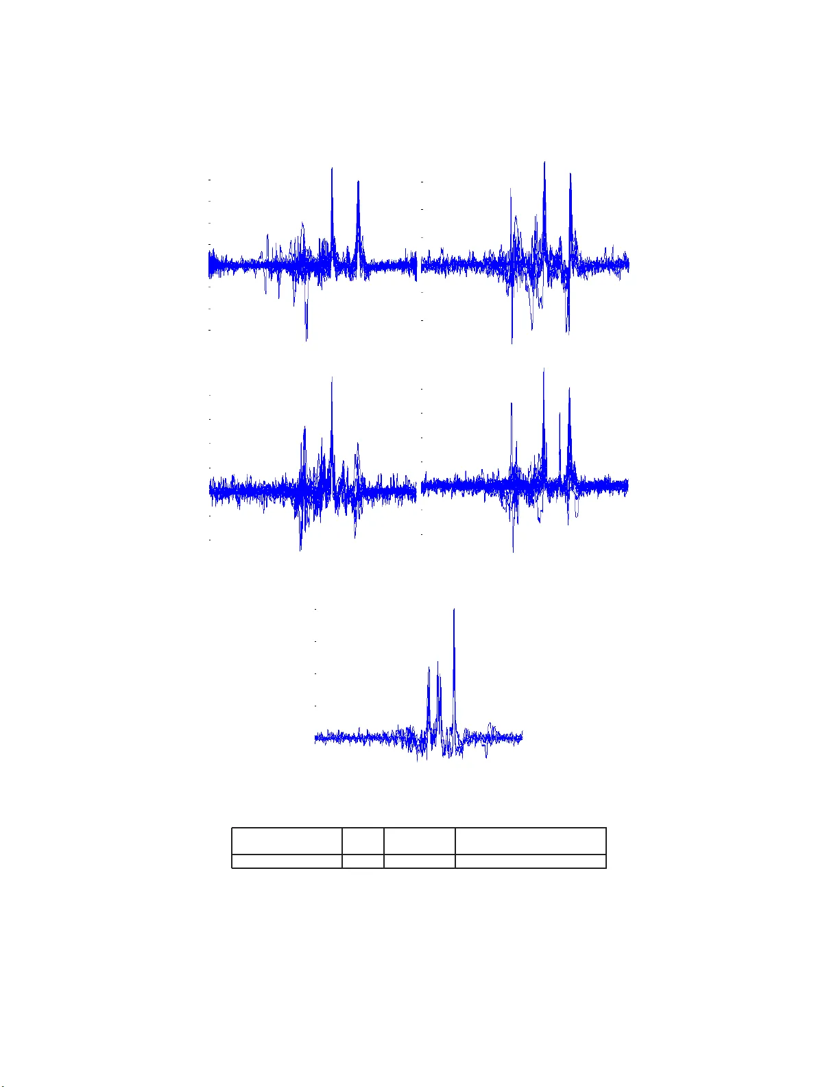
k F 10 k 2 L 2 ( γ C ) ≥ r . F rom the pr eceding prop o s ition, uniformly on a ll the p ossible v alues o f µ 1 and µ 0 , the lea rning err o r a nd the exces s risk can converge to zer o only if n p tends to 0. Recall that if no a priori as sumption is done o n m 10 , ¯ m 10 is the b est estimator (according to the mean square error) of m 10 . Also, as in the estimation of a high dimensional vector problem (such as those describ ed in ([ 9 ])), one should make a more restrictive hypothesis on m 10 . W e will supp ose, in Sectio n 5 , that if ( a k ) k ≥ 0 are the co efficients of C − 1 / 2 m 10 in a well chosen ba sis, then P k ≥ 0 a q k ≤ R q for 0 < q < 2. Pr o of. As in the preceding pro po sition, we will use inequality ( 13 ). Also it is sufficient to show the following E [ | α | ] ≥ ar c c os  1 √ p − 3 ( √ n k F 10 k L 2 ( γ C ) + 1)  where α is defined by ( 5 ). Because the function ar c cos is dec r easing and concav e on [0 , 1], it suffices to obtain E " |h F 10 , ˆ F 10 i L 2 ( γ C ) | k F 10 k L 2 ( γ C ) k ˆ F 10 k L 2 ( γ C ) # ≤ 1 √ p − 3 ( √ n k F 10 k L 2 ( γ C ) + 1) . (17) On the o ther ha nd, E " |h F 10 , ˆ F 10 i L 2 ( γ C ) | k F 10 k L 2 ( γ C ) k ˆ F 10 k L 2 ( γ C ) # ≤ E " k F 10 k L 2 ( γ C ) k ˆ F 10 k L 2 ( γ C ) # + E " |h F 10 , ˆ F 10 − F 10 i L 2 ( γ C ) | k F 10 k L 2 ( γ C ) k ˆ F 10 k L 2 ( γ C ) # ≤ E " k F 10 k 2 L 2 ( γ C ) k ˆ F 10 k 2 L 2 ( γ C ) # 1 / 2   1 + E " h F 10 , ˆ F 10 − F 10 i 2 L 2 ( γ C ) k F 10 k 2 L 2 ( γ C ) # 1 / 2   , where this last inequality results from Cauch y-Sch w artz. Recall that ˆ F 10 = F 10 + C − 1 / 2 √ n ξ , where ξ is a s tandardised gaussian random vector of R p . Also , we easily obtain, E " h F 10 , ˆ F 10 − F 10 i 2 L 2 ( γ C ) k F 10 k 2 L 2 ( γ C ) # 1 / 2 = 1 √ n , and k F 10 k 2 L 2 ( γ C ) k ˆ F 10 k 2 L 2 ( γ C ) = k √ nC 1 / 2 F 10 k 2 R p k √ nC 1 / 2 F 10 + ξ k 2 R p . The rest o f the pro o f follows fr om the following simple fact which is a con- sequence of the Co chran Theorem a nd a classical ca lculation on χ 2 random imsart-g eneric ver. 2007/12/10 file: article-fina l1.tex date: Octobe r 24, 2018 R. Gir ar d/High dimensional gaussian classific ation 14 v ariables: Let σ > 0, β ∈ R p , X a gaussia n r andom vector of R p with mean β and cov aria nce I p . Then E  1 k X k 2 R p  ≤ 1 p − 3 . 2.3. Case wher e k F 10 k L 2 ( γ C ) diver ges: wel l sep ar ate d data. W e s hall now rapidly consider the case when the data a r e well sepa rated: the case where k F 10 k L 2 ( γ C ) diverges. In the next theorem, we assume that p tends to infinity . Theorem 2. 2. Su pp ose that 0 < α < π / 2 ( α is define d by ( 5 )), and that cos( α ) k F 10 k L 2 ( γ C ) → ∞ when p tends to infinity. We then have R →    0 si lim inf p →∞ 2 | d 0 | |h F 10 , ˆ F 10 i L 2 ( γ C ) | < 1 b ≥ 1 8 si lim sup p →∞ 2 | d 0 | |h F 10 , ˆ F 10 i L 2 ( γ C ) | > 1 when p → ∞ . This theorem is prov ed in Sectio n 7 . In the case of w ell separated data it is obvious tha t the o ptima l rule will p er form p erfectly . Theo rem 2.2 s hows that for a g iven estimator ˆ F 10 one should c heck that the proba bilit y to have lim inf p →∞ 2 | d 0 | |h F 10 , ˆ F 10 i L 2 ( γ C ) | > 1 is small enough. 3. Q uadratic p erturba tion of quadratic rule 3.1. Main r esults and r emarks ab out the infini te dimensional setting In the cas e where C 1 6 = C 0 , L 10 ( x ) = L Q 10 ( x ) is a p olynomial function of degree t wo on R p : L Q 10 ( x ) = − 1 2 h A 10 ( x − s 10 ) , x − s 10 i R p + h G 10 , x − s 10 i R p − c, (18) where A 10 = C − 1 1 − C − 1 0 , G 10 = S m 10 , (19) S = C − 1 0 + C − 1 1 2 , c = 1 8 h Am 10 , m 10 i R p − 1 2 log | det( C − 1 0 C 1 ) | , m 10 and s 10 are defined by ( 3 ). Remark 3.1. The e qu ation ( 19 ) giving L Q 10 ( x ) c an b e mo difie d using the fact that A 10 = 1 2  C − 1 / 2 1 W 10 C − 1 / 2 1 − C − 1 / 2 0 W 01 C − 1 / 2 0  wher e W ij = I − C 1 / 2 i C − 1 j C 1 / 2 i . (20) imsart-g eneric ver. 2007/12/10 file: article-fina l1.tex date: Octobe r 24, 2018 R. Gir ar d/High dimensional gaussian classific ation 15 This mo dific ation has two advantages. It involves W ij which play an imp ortant r ole in the infin ite dimensional fr amework (se e r emark 3.2 ). On the other hand, it involves W 10 as much as W 01 which c an le ad in pr actic e (while estimating A 10 ) to a symmet ric pr o c e dur e that do es not give mor e imp ortanc e to any gr oup. In the clas sification pro blem, a p olynomia l of degree tw o b L Q 10 ( x ) is used as a substitute for L 10 . W e decide tha t X co mes fr o m cla ss o ne if it b elong s to ˆ V = n x ∈ R p tq b L Q 10 ( x ) ≥ 0 o , (21) The following theorem gives o ur solution to Problem 1 . Theorem 3.1. L et γ b e a gaussian me asur e on R p . Supp ose that L Q 10 is a p olynomial of de gr e e two on R p and that we have k L Q 10 k L 2 ( γ ) ≥ r for r > 0 . Then, for al l q ∈ ]0 , 1[ , ther e exists c 1 ( r , q ) > 0 su ch that R ( 1 ˆ V ) ≤ c 1 ( r , q ) kL Q 10 − b L Q 10 k q/ 3 L 2 ( γ ) , (22) wher e ˆ V is given by ( 21 ) and R by ( 8 ). W e emphasise the fact that c 1 ( r , q ) dep ends only r and q . In par ticular it do es not depend on the dimension p of the problem. The pr o of of this Theorem is giv en in Section 8 . It is implicitly infinite dimensional, and the prec e ding theorem co uld have b een stated in an infinite dimensional fr a mework. W e do not w a nt to introduce this complicated framework and we refer to [ 8 ] for an int ro duction to the sub ject. The infinite dimensio nal fra mework highlights a particular asp ect o f the problem that is c o ntained in the following remar k. Remark 3.2. [infinite dimensional fr amework] W hen X is a sep ar able Hilb ert sp ac e (it c an also b e a sep ar able Banach sp ac e in t he c ase of LDA) two gaussian me asur es γ C 1 ,µ 1 and γ C 0 ,µ 0 that ar e not e qu ivalent ar e ortho gonal. If t hese me asu r es ar e ortho gonal then t he observe d data fr om the t wo classes ar e p erfe ct ly sep ar ate d and C ( g ∗ ) = 0 . In this c ase one c an hop e to obtain C ( g ) = 0 for a r e asonable classific ation rule g (Even if it is not trivial, se e The or em 2.2 in the line ar c ase). A ne c essary and sufficient c ondition for these me asur es to b e e quivalent is that m 10 = µ 1 − µ 0 ∈ H ( γ C 1 ,µ 1 ) = H ( γ C 0 ,µ 0 ) , (23) and W 10 = I − C 1 / 2 1 C − 1 0 C 1 / 2 1 ∈ H S ( X ) , (24) wher e H ( γ ) is t he r epr o ducing Kernel Hilb ert S p ac e asso ciate d with a gaussian me asur e γ and H S ( X ) is the sp ac e of Hilb ert Shmidt op er ators with values in X (se e c or ol la ries p293 in [ 8 ]). In p articular, the eigenvalues of W 10 ar e in l 2 . In the c ase wher e t hey ar e e quivalent, one c an define L 10 as a limit (almost sur ely and L 2 ) of its finite dimensional c oun terp art. This c an also b e understand as me asur able and squar e d inte gr able (with r esp e ct to γ C 1 ,µ 1 ) p olynomials of de gr e e two in X (se e Chapter 5 . 1 0 in [ 8 ]). imsart-g eneric ver. 2007/12/10 file: article-fina l1.tex date: Octobe r 24, 2018 R. Gir ar d/High dimensional gaussian classific ation 16 3.2. Comment and Cor ol lary . Supp os e b L Q 10 ( x ) is defined substituting ˆ G 10 , ˆ s 10 ˆ A 10 and ˆ c to G 10 , s 10 A 10 and c in ( 18 ). If we note δ 0 = ˆ c − c + D ˆ G 10 + ( ˆ A ∗ 10 + ˆ A 10 )( ˆ s 10 − s 10 ) , ˆ s 10 − s 10 E R p , (25) ( A ∗ is the transp ose of a matrix A ) δ L = ˆ G 10 − G 10 + ( ˆ A ∗ 10 + ˆ A 10 )( ˆ s 10 − s 10 ) (26) and δ Q = ˆ A 10 − A 10 , (27) we then g et, by straightforward calculation: ∀ x ∈ R p b L Q 10 ( x ) = L Q 10 ( x ) + δ 0 + h δ L , x − s 10 i R p − 1 2 h δ Q ( x − s 10 ) , x − s 10 i R p . (2 8 ) Also, a re result are ab out q uadratic p erturbations of quadratic rules. The following coro llary of Theorem 3.1 is ea sier to use. Corollary 3.1. L et X = R p and C b e a s ymm et ric p ositive definite matrix on R p . S u pp ose t hat ther e exists r > 0 su ch that kL 10 k 2 L 2 ( γ C,s 10 ) > r . Then, for 1 ˆ V given by ( 21 ) and for al l 0 < q < 1 t her e exists c 1 ( r , q ) > 0 su ch that: R ( 1 ˆ V ) ≤ c 1 ( r , q )  1 2 k C ( A 10 − ˆ A 10 ) k 2 H S ( R p ) + k C 1 / 2 δ L k 2 R p +2 δ 2 0 + 1 2 trace 2 ( C ( A 10 − ˆ A 10 ))  q/ 3 , wher e δ L is given by ( 26 ) and δ 0 by ( 25 ) . Pr o of. Let us recall that δ Q is g iven b y ( 27 ). W e hav e kL 10 − b L 10 k 2 L 2 ( γ C,s 10 ) = k 1 2 ( δ Q ( x ) − E γ C [ q δ Q ( X )]) − h δ L , x i R p − ( δ 0 − 1 2 E γ C [ q δ Q ( X )]) k 2 L 2 ( γ C ) ≤ 1 4 V ar ( q C 1 / 2 δ Q C 1 / 2 ( ξ )) + V ar ( h C 1 / 2 δ L , ξ i R p ) + 2 δ 2 0 + 2 E 2 γ C [ q C 1 / 2 δ Q C 1 / 2 ( ξ )] ( ξ ❀ γ I p , 0 , no te that there is equa lity here) = 1 2 k C 1 / 2 δ Q C 1 / 2 k 2 H S ( R p ) + k C 1 / 2 δ L k 2 R p + 2 δ 2 0 + 1 2 trace 2 ( C 1 / 2 δ Q C 1 / 2 ) . imsart-g eneric ver. 2007/12/10 file: article-fina l1.tex date: Octobe r 24, 2018 R. Gir ar d/High dimensional gaussian classific ation 17 3.3. Comp ar ison of this r esult with those obtaine d for LDA. The prece ding theor em and its co r ollary ar e less powerful than those o btained for the LDA pr o cedure and some co njectures might b e made in a par allel with Theorem 2.1 . In this theorem and in Theore m 2.2 , bo th co ncerning linea r r ules, we explained and quantified how par ameter estimation errors are less impo rtant when k F 10 k L 2 ( γ C ) is large. This observ ation was based on the pres ence of a ter m exp onentially decreasing with k F 10 k L 2 ( γ C ) in the quantities which determine the upper b ound to the learning error (a nd as a conseq uence the excess risk). In Theorem 3.1 concer ning Q D A pro cedur e, we did no t obtain that type of term. Nevertheless, Remark 3.2 (more precis e ly the relation this leads to equiv alence of the mea s ures) allow us to co njecture that s uch a term e x ists. W e also hav e to clarify the hypothesis under which the nor m of L Q 10 is low er bo unded. Le t us recall tha t this hypothesis guar anties that the co ns tant c 1 in equation ( 22 ) is independent of the parameter s of the problem. In a pa rallel with the results obtained for the pro cedur e LD A the lower b ound tha t is required for the nor m of L Q 10 corres p o nds to the a ssumption that the tw o groups co nsidered can a lwa ys be distinguished. W e b elieve that even if this hypo thesis is natural, it is deeply linked with e rror measure that is used in our proo f: the lear ning error . Hence, it is obvious that the ex cess risk is s ma ll when the data cannot be disting uished (see Section 6 for a fuller discussion) but our res ult do es no t reflect this fact. W e do not discuss the estimation of G 10 which le a ds to the sa me analysis as that for F 10 in the cas e o f a linear rule . Let us now discuss the estimation of W 10 (and W 01 ). 3.4. Thr esholding estimation of an op er ator and l i ne arisation of a pr o c e dur e. Recall that W 10 is a symmetr ic matrix . Supp o se we k now an o rthonormal bas e in which it is dia gonal. Let λ 10 = ( λ 10 i ) i =1 ,...,p be the vector o f its eigenv alues. T o build the estimator ˆ W 10 of W 10 , we hav e to es tima te its eigenv alues. It remains to meas ure the lea rning erro r and hence the estimation error of the eigenv alues vector in l 2 norm. Supp ose that p tends to infinity . W e will recall later that if the measure o f class 0 and 1 tend to equiv alent gaussian measur e in a sepa rable Hilb ert spa ce, then W 10 tends to b e Hilb ert-Schmidt. This means that λ 10 stays in l 2 ( N ). Once again, if λ 10 has co efficients decreasing sufficiently fast, the thresho lding estimatio n s hould b e used. This thres holding es timation is no lo ng er a reduction of the dimension of the space in which the r ules acts, but b ecomes a linea risation of the classificatio n rules - It can b e in terpreted as a r eduction of the dimension of the space in which the used rule lives- Indeed, let ˆ W 10 = P l i =1 ˆ λ 10 i e i ⊗ e i for l ≤ p and ( e i ) i =1 ,...,p be an orthonorma l bases of R p , we hav e: b L Q 10 = l X i =1 ˆ λ 10 i h e i , x − ˆ s 10 i 2 R p + g ( x ) , imsart-g eneric ver. 2007/12/10 file: article-fina l1.tex date: Octobe r 24, 2018 R. Gir ar d/High dimensional gaussian classific ation 18 Figure 1 . Sep ar ation of the data in a dir e ction wher e the v arianc es ar e differ ent . The two gr oups c an b e identified with their el lip soids of c onc ent r ation: a horizontal el lipsoid and a vertic al el lipso id. the two gr oups have the same me an, but differ e nt c ovarianc e, which makes the data q uite wel l sep ar ate d. One c an t ake advantage of t his sep ar ation only if a quadr atic rule is use d. imsart-g eneric ver. 2007/12/10 file: article-fina l1.tex date: Octobe r 24, 2018 R. Gir ar d/High dimensional gaussian classific ation 19 where g ( x ) is affine and defined on R p . In this cas e, the plug-in rule is affine in a subspace of dimension p − l a nd q uadratic in the subspace of dimension l spanned by ( e i ) i =1 ,...,l . Let us note that b eca us e W 10 = I − C − 1 / 2 1 C 0 C − 1 / 2 1 , setting the eige n v alues of ˆ W ij to zero in a subspace of R p , is equiv alent to choosing a subspace in which the cov aria nce matrices C 1 and C 0 are ”close enough”. In this subs pa ce, one ca n suppo se that C 1 equals C 0 . The cla ssification rule, in this subspace, is linear . Figure 1 illustra tes the case w her e the eigenv a lues of W 10 are big enough and why a qua dratic rule is b etter in tha t c a se. 4. Cl assification pro cedure in hi gh di m ension: a wa y to solve Problem 2 4.1. Intr o du ction. In this sec tio n, we give a pra ctical metho d of classifica tion for gauss ia n data in high dimension and hence pr esent our contribution to Problem 2 . Note that if we only treat the binar y cla ssification problem, it is easy to extend our pro cedure to the ca se of K classes as we hav e do ne in [ 15 ]. Reca ll that we are giv e n n 1 observ ations from P 1 and n 0 observ ations from P 0 . W e will no te n = n 1 + n 0 . W e supp ose tha t each of the n k vectors of gr oup k is comp ose d o f the p fir st wa velet co efficient (see [ 20 ]) of a random curve fro m X = L 2 [0 , 1] whic h is a realisatio n o f a gaussian r a ndom v aria ble P k = γ C k ,µ k of unknown mean a nd cov aria nce. Recall that a lea rning rule can b e defined by a partition of R p . W e co nstruct this partition ˆ V , R p \ ˆ V of R p with the use of a frontier functions b L 10 : ˆ V = n x ∈ R p : b L 10 ( x ) ≥ 0 o , (29) which s hould b e given in the s equel. W e divide here the presentation into tw o parts. In the first part, we g ive a theoretical result in the ca se where the cov ariance matrices are supp osed to b e known. In the second part, we give the metho d that is used when the co v ariances are unknown. W e k eep the notation of the preceding sectio ns. In the ca s e of LDA pro cedure, m 10 = µ 1 − µ 0 F 10 = C − 1 m 10 , s 10 = µ 1 + µ 0 2 , and in the cas e of the QDA pr o cedure, G 10 = 1 2 ( C − 1 1 + C − 1 0 ) m 10 , A 10 = C − 1 1 − C − 1 0 . 4.2. Case of known and e qual c ovarianc e: pr o c e dur e and the or etic al r esult. Notation and assumpti ons. Let ¯ µ k be the empirical mea n o f the lea rning data ( X ik ) i =1 ,...,n k of clas s k . W e supp os e here tha t the cov ariance of group 0 and 1 equal C , and that s 10 is known. The separ ation fr ontier b etw e e n the imsart-g eneric ver. 2007/12/10 file: article-fina l1.tex date: Octobe r 24, 2018 R. Gir ar d/High dimensional gaussian classific ation 20 t wo g roups is a ffine a nd F 10 is the only unknown parameter . W e supp ose that the lear ning set is made of n 1 = n 0 = n ( p ) / 2 p -dimensional vectors. W e g ive a metho d to c onstruct an estimator of F 10 and g ive theoretical results when n ( p ) tends then to infinity m uch more s lowly than p . F or q > 0, the ball l q p ( R ) is comp osed of the vectors θ ∈ R p such that p X i =1 | θ i | q ≤ R q . W e will note Ω p (Θ( R ) , r ) = { ( x, y , C ) ∈ R p × R p × C p such that (30) C − 1 / 2 ( x − y ) ∈ Θ ( R ) a nd k C − 1 / 2 ( x − y ) k R p ≥ r o where C p is the set of symmetric definite p ositive matric e s in R p . If ( µ 0 , µ 1 , C ) ∈ Ω p (Θ( R ) , r ), we w ill note D ( ˆ L 10 ) = C ( 1 ˆ V ) − C ( 1 V ) , (31) where ˆ V is given by ( 29 ) and V is given b y ( 2 ). The Pro cedure. The plug -in rule affect the obser v ation X to class 1 if it belo ngs to ˆ V defined by ( 29 ) where b L 10 = h ˆ F 10 , X − s 10 i R p . W e estimate F 10 = C − 1 m 10 by ˆ F 10 = C − 1 ˆ m 10 , where the co efficients o f C − 1 / 2 ˆ m 10 are g iven by  y 10 l 1 | y 10 l | >λ F DR 10  l =1 ,...,p , where y 10 l =  C − 1 / 2 ( ¯ µ 1 − ¯ µ 0 )  l =1 ,...,p , and λ F DR 10 is chosen by the Benja mini a nd Ho cheberg pro cedure [ 4 ] for the control of the false discov er y rate (FDR) of the following m ultiple h yp otheses: ∀ l = 1 , . . . , p H 0 l : E [ y 10 l ] = 0 : V er sus H 0 l : E [ y 10 l ] 6 = 0 (3 2 ) W e r ecall tha t this pro cedur e is the following. The ( | y 10 l | ) l are ordered in de- creasing order: | y 10(1) | ≥ · · · ≥ | y 10( p ) | and λ F DR 10 = | y 10( k F D R 10 ) | where k F DR 10 = max ( k ∈ { 1 , . . . , p } : | y 10( k ) | ≥ s 1 n ( p ) z  b p k 2 p  ) , z ( α ) is the quantile of order α o f a sta ndardized ga ussian random v a riable and b p ∈ [0 , 1 / 2[ is low er bounded b y c 0 log p where c 0 is a p ositive constant (which do es no t dep e nd o n p . imsart-g eneric ver. 2007/12/10 file: article-fina l1.tex date: Octobe r 24, 2018 R. Gir ar d/High dimensional gaussian classific ation 21 Theoretical result Theorem 4.1. L et R > 0 , and q ∈ ]0 , 2[ . L et ˆ V b e define d by ( 29 ) and η p = p − 1 q R p n ( p ) . Supp ose that p tends to infinity. If η q p ∈ [ log 5 ( p ) p , p − δ ] for δ > 0 , then, for r > 0 , we have sup ( µ 0 ,µ 1 ,C ) ∈ Ω p ( l q ( R ) ,r ) E P ⊗ n h D p ( ˆ L 10 ) i ≤ 1 + o p (1) r   √ 2 log 1 / 2  p R q n ( p ) q/ 2  Rn 1 / 2 ( p )   2 − q 2 , wher e D p is t he exc ess risk as define d by ( 31 ), and P ⊗ n is t he law of t he le arning set. Pr o of. The cov a r iance matrix of the vector C − 1 / 2 ( ¯ µ 1 − ¯ µ 0 ) eq ua ls I p 1 n ( p ) . W e then have to use succes sively The o rem 2.1 (of this article), Theo r em 1 . 1 o f Abramovic h et .al [ 1 ], and Theore m 5 po int 3 b. of Donoho and Jo hnstone [ 11 ] to b e a ble to wr ite, ∀ r > 0 : sup ( µ 0 ,µ 1 ,C ) ∈ Ω p ( l q ( R ) ,r ) E P ⊗ n h D 2 p ( ˆ L 10 ) i ≤ 1 + o p (1) r 2   √ 2 log 1 / 2  p R q n ( p ) q/ 2  Rn 1 / 2 ( p )   2 − q . This inequa lity leads to the result by the use of the J ensen inequality: E P ⊗ n h D p ( ˆ L 10 ) i ≤ E P ⊗ n h D 2 p ( ˆ L 10 ) i 1 / 2 . Comments. Let us ma ke a few r emarks o n this r esult. 1. The r ate of conv erge nce is fas ter when q is close to 0, and s low er when it is close to 2. This leads us to consider the spar sity of C − 1 / 2 ( µ 0 − µ 1 ), and makes the use of the w av elet basis attractive. On the one hand, it transforms a wide class of curves in to spar se vectors and on the other hand, it almost diagona lises a wide class of cov a riance op erato rs. 2. W e could obta in the same sp eed with a universal threshold (i.e with the threshold λ U = 1 n ( p ) p 2 log( p ) ). In this ca se, the constan t 1+ o p (1) r 2 would not b e that go o d (cf [ 1 ]). 3. W e are not aw ar e of any r esults concerning the conv ergence of any cla ssifi- cation pr o cedure in this framework (the high dimensional g aussian fra me- work with the s e t of po ssible para meter deter mined by Ω p ). Indeed we do not make any str o ng assumption on C . Bick el and Le v ina [ 6 ] as well as F an and F an [ 12 ] supp ose in their work that the ratio b etw een the highes t and the low es t eig env alue is lo w er a nd upp er- b o unded. Even if o ur Theorem do esnot tr eat the case wher e C is unknown the hypotheses we us e seems more na tural. Let us reca ll tha t if Y is a gaussia n random v ar iable with imsart-g eneric ver. 2007/12/10 file: article-fina l1.tex date: Octobe r 24, 2018 R. Gir ar d/High dimensional gaussian classific ation 22 v alues in a Hilber t Space, then the cov ariance op era tor is neces s arily nu- clear. Also, the assumption used by the ab ove mentioned author s does not allow us to consider gaussian measures with supp ort in a Hilbe r t space. 4. Finding the sig nificant comp onent of the nor mal vector F 10 defining the optimal separating hype rplan is equiv a le nt with finding the significa n t contrast in a m ultiv a riate ANOV A. Hence, c o ntrolling the exp ected fals e discov er y ra te in this ANO V A is sufficient to get a go o d cla ssification rule. 4.3. The c ase of diff er ent un know n c ovarianc es F or the r est of this sectio n, if k ∈ { 0 , 1 } , ¯ µ k will b e the empirical mean o f the Learning data of class k . W e are going to use a diagonal es timator ˆ C k of the cov aria nce ma trix C k . The diag o nal elemen ts of ˆ C k will b e ( ˆ σ 2 kq ) q =1 ,. ..,p . F or q ∈ { 1 , . . . , p } , k ∈ { 0 , 1 } , ˆ σ 2 kq will we the unbiased version of the empir ic al v ariance o f feature q of the o bs erv ations ( X ikq ) i =1 ,...,n k of class k . W e will note ˆ s 10 = ( ¯ µ 1 + ¯ µ 0 ) / 2 . The classifica tion rule used choos es that X ∈ R p comes from the class k if X belo ngs to ˆ V k given by ( 29 ) and ˆ L 10 = − 1 2 h ˆ A 10 ( x − ˆ s 10 ) , x − ˆ s 10 i R p + h ˆ G 10 , x − ˆ s 10 i R p − ˆ c 10 , where the quantities of this equation will b e given in w ha t follows. for all (1 , 0) ∈ { 1 , . . . , K } 2 , 1 6 = 0, we now giv e ˆ G 10 (equation ( 33 )), ˆ A 10 (equation 34 ), and ˆ c 10 (equation 35 ). W e estimate G 10 = 1 2 ( C − 1 1 + C − 1 0 ) m 10 by ˆ G 10 =   1 √ 2 1 ˆ σ 2 1 q + 1 ˆ σ 2 0 q ! 1 / 2 y 10 q 1 | y 10 q | >λ F DR 10   q =1 ,. ..,p (33) where y 10 q = 1 √ 2 1 ˆ σ 2 1 q + 1 ˆ σ 2 0 q ! 1 / 2 ( ˆ µ 1 q − ˆ µ 0 q ) , and λ F DR 10 is c ho sen by the Benjamini and Ho cheberg pr o cedure. This pro cedure is the following. Let V ar 0 ( y ij q ) b e the v ar iance of y 10 q calculated under the hypothesis that µ 1 q = µ 0 q . The ter m 1 + ˆ σ 2 1 q / ˆ σ 2 0 q 2 n 1 + 1 + ˆ σ 2 0 q / ˆ σ 2 1 q 2 n 0 is an estimation of this v ariance when σ 2 kq ( k = 0 , 1) are known a nd equal to ˆ σ 2 kq . In pra ctice, we substitute these terms for V ar 0 ( y 10 q ). The real ( | y 10 q | / q V ar 0 ( y 10 q )) q =1 ,. ..,p imsart-g eneric ver. 2007/12/10 file: article-fina l1.tex date: Octobe r 24, 2018 R. Gir ar d/High dimensional gaussian classific ation 23 are o r dered by decreasing order: | y 10(1) | / q V ar 0 ( y 10(1) ) ≥ · · · ≥ | y 10( p ) / q V ar 0 ( y 10( p ) ) | and λ F DR 10 = | y 10( k F D R 10 ) | where k F DR 10 = max    k : | y 10( k ) | ≥ s 1 + ˆ σ 2 1( k ) / ˆ σ 2 0( k ) 2 n 1 + 1 + ˆ σ 2 0( k ) / ˆ σ 2 1( k ) 2 n 0 z  b p k 2 p     , z ( α ) is the quantile of order α o f a sta ndardized ga ussian random v a riable and b p ∈ [0 , 1[ is as in the preceding algo rithm. In practice, we choo s e b p = 0 . 01, but one could k eep a part o f the learning set to lea rn the be s t v alue of b p . Note that in the applica tion we hav e in mind, the learning se t is to o small to b e divided. In addition, the choice of b p , in view o f Theorem 4.1 do es not determine the p erfor mances o f the algor ithm. In pra c tice the differe nc e of classificatio n error b etw een the choices b p = 0 . 01 a nd b p = 0 . 05 for example, is not imp or tant. This first part of the metho ds constitute a dimensio n re duction. Indeed, the only co ordina tes of ( ˆ G 10 q ) q =1 ,. ..,p that are k ept non n ull are those for which | y 10 q | ≥ λ F DR ij . The linea r application asso cia ted with ( ˆ G 10 q ) q =1 ,. ..,p only acts in k F DR 10 directions. Let us a lso note that if we extend our pro cedure to a m ul- ticlass proc e dure, for tw o couples of classes ( i, j ) 6 = ( l, m ), the cor resp onding estimations G ij and G lm might b e based on different dimension reduction. Remark 4.1. Th e test ing pr o c e du re use d c an b e analyse d as a ”vertic al” ANOV A that r eve als the inter esting dir e ction 1. in which classific ation should b e done (with thr esholding estimation of G 10 ) 2. in which classific ation should b e quadr atic (with thr esholding estimation of A 10 ). The matrix A 10 is estimated b y a diagonal matrix with diag onal elements given by ˆ a 10 q = 1 ˆ σ 2 1 q − 1 ˆ σ 2 0 q ! 1 | w 10 q |≥ η F D R 10 , where w 10 q = ˆ σ 2 1 q − ˆ σ 2 0 q , q = 1 , . . . , p, (34) and the threshold η F DR 10 is chosen with the same type o f pr o cedure as the one used to find λ F DR 10 . Let V ar 0 ( w 10 q ) be the v ariance of w 10 q under the h yp o thes is that σ 1 q = σ 0 q . The term 2 ˆ σ 4 1 q n 1 − 1 + 2 ˆ σ 4 0 q n 0 − 1 is an estimation of it that we use in practice. The r eal num b er s ( | w 10 q / p V ar 0 ( w 10 q ) | ) q are ordered by decreasing order: | w 10(1) / q V ar 0 ( w 10 p ) | ≥ · · · ≥ | w 10( p ) / q V ar 0 ( w 10 p ) | and η F DR 10 = | w 10( k F D R 10 ) | imsart-g eneric ver. 2007/12/10 file: article-fina l1.tex date: Octobe r 24, 2018 R. Gir ar d/High dimensional gaussian classific ation 24 where k F DR 10 = max    k : | w 10( k ) | ≥ s 2 ˆ σ 4 1( k ) n 1 − 1 + 2 ˆ σ 4 0( k ) n 0 − 1 z  b p k 2 p     . This part of the metho d constitutes a linearisatio n o f the rule. Indeed, the directions q ∈ { 1 , . . . , p } in which ˆ a 10 q is 0 are the directions in which the cla s- sification rule betw een the g roups 1 and 0 is linear. In the other dir e c tions, the rule is qua dratic. The use of this metho ds is still motiv ated by Theo rem 4.1 and the theorems used in its pro of, but it nee ds additional theoretical justification. W e will finally note: ˆ c 10 = p X q =1 1 | w 10 q |≥ η F DR 10  1 8 ˆ a 10 q ( ¯ µ 1 q − ¯ µ 0 q ) 2 + 1 2 log | det( ˆ σ − 1 0 q ˆ σ 1 q ) |  . (35) 5. Appl ication to medi cal data and the TIMIT database W e are g oing to study the p erfor ma nce o f the given pro cedure. With that a im, we compa r e our metho d with the one g iven by Rossi and Villa [ 22 ] on the database TI MIT. W e then use tes t o ur pro cedure on medical da ta. 5.1. Comp ar ison of our metho d with the one of R ossi and Vil la i n the c ase of two class classific ation Rossi and Villa use a supp or t vector machine (SVM) with differe n t t ypes of kernels. Recall that the SVM pr o cedure is to cons tr uct an affine frontier function f given by f ( x ) = h w, x i R p + b, where w a nd b a re solutio ns of a n optimiza tion pro blem of the fo llowing type: min w, b,ξ k w k 2 R p + C N X i =1 ξ i under y i ( h w, x i i R n + b ) ≥ 1 − ξ i , ξ i ≥ 0 i = 1 , . . . , n where ( x i , y i ) i =1 ,...,n are the couples (observ ations, lab e ls) of the learning set. The TIMIT databa se has notably been studied b y Ha stie et al. [ 18 ]. This database includes phonemes ”a a” and ” ao ” pr onounced by many differen t per - sons. The co rresp onding re c ords a r e curves observed at a fine enough sampling frequency . More precisely , one curve is a p -dimensional vector with p = 256. The learning set is comp osed of 519 ”aa” and 759 ” ao ” and the test s et is comp osed of 176 ”aa” and 263 ”ao” . Also , the curves ( x i ) i =1 ,..., 519 are those which corres p o nd to the pronunciation of phoneme ” aa” and the label y i = 0 is as s o ciated to them. The lab e l ”1” is asso cia ted to the other curv es which corres p o nd to the pronunciation of phoneme ” a o ”. The metho d o f Ro ssi a nd Villa g ives almost the same results as ours: 2 0% o f classification mistakes. imsart-g eneric ver. 2007/12/10 file: article-fina l1.tex date: Octobe r 24, 2018 R. Gir ar d/High dimensional gaussian classific ation 25 5.2. Applic ation to me dic al data The medical pr oblem is the following. In Mag netic resona nc e imag e ry , one can obtain spectra characterizing tissues loca lized in some area of the br ain. The sp ectra obtained can b e used to characterize tumors . Unfortunately , even for a sp ecia lis t, it is hard to define a go od r ule to a sso ciate the name of a tumor with a g iven sp ectra. Some spec tra hav e be e n o btained on identified tumors. W e hav e b een given these sp ectra. In order to hav e enough s p ectr a in o ur lea rning set, we reta ined five groups o f sp ectr a (some of them reg rouping many tumors). The glio bla stomes of the fir st type 1 , the glioblas tomes o f the second t ype , the Meningiomes, the Metastase s and the healthy tissues. The databa s e provided by the sp ecialis ts contains 21 gliobla s tomes of first type, 9 g lioblastomes of second t yp e , 16 M´ eningiomes, 18 m´ etastases and 9 healthy tissues, that is, 7 5 s p ectr a sampled at 1024 p oints. W e giv e the plot of the sp ectra considered in Figure 2 . In order to test our proce dur e, we used a str a tegy o f t ype ”leave on out”. Figure 4 leads us to an exp erimental confir mation tha t in the case of tw o class classification, the chosen dimension is a go o d one. W e tested differen t co nfigurations s ummarized in the table Figure 3 . The classification erro r rate is s till s ignificant, but the reduction dimensio n pro cedure provides a r eduction of the error ra te (Reca ll that in the case of 4 gro ups having equal a priori probability a r ule that w ould gue s s randomly the type of tumor would have an er ror rate of 75%). Ther e a re t wo reaso ns for this mo derate per formances. Roughly , theor etical physic predicts that a sp ectrum a s so ciated with a g iven tumor, for example a Glioblastome, is a r andom v aria ble y = ( y q ) q =1 ,. ..,p that has a quite s ma ll v ar iability . Also, we shuold b e able to separate easily sp ectra asso ciated with different gr oups. Unfor tuna tely , in practice, the instrument ation leads to a measur ement of sp ectra z = ( z q ) q =1 ,. ..,p having complex v alues and for which ther e exists a sequence of angles ( ψ q ) q =1 .. .,p such that: ∀ q ∈ { 1 , . . . , p } y q = ℜ ( e iψ q z q ) . This sequence of a ngles is unknown. The theoretical physics o f instrumentation shows tha t there a re t w o r eal ( a, b ) such that ∀ q ∈ { 1 , . . . , p } ψ q = aq + b. Metho ds to obtain a a nd b are not sufficiently efficien t, but this repr e sents an active field o f research. W e chose to ask the physicians to change the phase manually in order to ha ve a homogeneous real pa r t of the s pectr a in a pa rticular group and we kept the r eal part of the sp ectra . The change of phase made by the physicians is not optimal and the residua l v aria tion of the phase c reates a certain disparity o f observed sp e ctra inside ea ch gro up. This disparity can b e seen Figure 2 . The incorpo ration o f the phase int o a cla ssification algorithm, 1 The group of Gli oblastomes has a to o large v ariability , also, we chose to divide it into t w o groups: first type and second t ype. These tw o types correspond to the presence of certain c hemical substances. imsart-g eneric ver. 2007/12/10 file: article-fina l1.tex date: Octobe r 24, 2018 R. Gir ar d/High dimensional gaussian classific ation 26 (a) 21 gli oblastomes A (b) 9 glioblastomes B (c) 16 Meningiomes (d) 18 metastases (e) 9 healthy tissues Figure 2 . Sp e ctr a of the le arning set Groups considered all all except Glioblastomes of fir s t t yp e Metastases and M eningiomes error rate 43 % 30 % 5% Figure 3 . Consider e d gr oups and err or r ate in e ach c ase. imsart-g eneric ver. 2007/12/10 file: article-fina l1.tex date: Octobe r 24, 2018 R. Gir ar d/High dimensional gaussian classific ation 27 Figure 4 . Classific ation e rr or r ate (in a two gro up pr oblem: M´ eningiomes v ersus Glioblas- tomes of first typ e) as a function of t he sele ct e d dimension. The dimension sele cted by our algorithm i s marke d by a b lack p oint in the Figur e. and the use of the complex nature of the data will be the ob ject of further studies. W e no te, how ever tha t these phase problems in the F ourier domain can be translated interestingly in the temp o ral domain. Finally , the learning s et is still to o small. W e hop e to see the size incr ease in the forthcoming years. 6. A mo re geom etric alternative measure of error: the l earning error 6.1. Definition and main r esul t W e hav e a lready defined the learning erro r to b e R ( g ) = P ( g ( X ) 6 = Y et g ∗ ( X ) = Y ) , which whe n Y ❀ U ( { 0 , 1 } ) equals R ( g ) = 1 2 ( P 1 ( g ( X ) 6 = 1 et g ∗ ( X ) = 1) + P 0 ( g ( X ) 6 = 0 et g ∗ ( X ) = 0)) . In other words, the lear ning er r or is the pr obability to misclassify X with g and to classify it cor rectly with g ∗ . The p o in t that motiv a tes the use of this err or is that 1. it le ads to a simple g eometric interpretation (mos tly used in the t w o follow- ing Sections) and hence it is used in all the further theore tical developmen t we will give; 2. it is not sensitive to the p ossible indis tinguishability o f the distributions P 0 and P 1 and it lea ds to low er bounds a s in Se c tio n 2 (see remark below). imsart-g eneric ver. 2007/12/10 file: article-fina l1.tex date: Octobe r 24, 2018 R. Gir ar d/High dimensional gaussian classific ation 28 It follows ea sily from C ( g ) − C ( g ∗ ) = P ( g ( X ) 6 = Y et g ∗ ( X ) = Y ) − P ( g ( X ) = Y et g ∗ ( X ) 6 = Y ) , that a classification rule g satis fies : C ( g ) − C ( g ∗ ) ≤ R ( g ) . (36) In the ga ussian case that is studied in this article, we prov ed the following theorem that gives a r everse inequality of ( 36 ). Theorem 6.1. L et g ∗ b e the optimal ru le in the binary classific ation pr oblem (as pr esente d in Se ction 1 ) . 1. If P 0 and P 1 have the same c ovarianc e C and r esp e ctive me ans µ 1 and µ 0 , then, for al l me asur able fu n ctions g : R p → { 0 , 1 } , we have: C ( g ) − C ( g ∗ ) ≥ min ( √ 2 π 2 ∗ 16 2 k C − 1 / 2 m 10 k R p e k C − 1 / 2 m 10 k 2 R p 8 R ( g ) 2 , R ( g ) 8 ) , wher e m 10 = µ 1 − µ 0 . 2. Le t c 1 > 0 and P ( c 1 ) b e t he set of c ouples ( P, Q ) of gaussian me asure on R p such t hat d 1 ( P, Q ) > c 1 . If ( P 1 , P 0 ) ∈ P ( c 1 ) then t her e ex ists a c onstant c ( c 1 ) > 0 (t hat only dep ends on c 1 ) such that C ( g ) − C ( g ∗ ) ≥ min  c ( c 1 ) R ( g ) 8 , R ( g ) 8  . Before we prov e this result, let us comment it. Comments. Let us no te that C ( g ) − C ( g ∗ ) ≤ 1 2 d 1 ( P 1 , P 0 ) . Also, in the ca se where d 1 ( P 1 , P 0 ) tends to 0, the excess risk do es not measure the differ ence b etw een g and g ∗ but the proximity o f P 1 and P 0 . The lear ning error is not sensitive to this scale phenomeno n, a s witness the following example. Example 6.1. L et µ ≥ 0 , P 1 = N ( µ, 1) and P 0 = N ( − µ, 1) . In this c ase, for al l a ∈ R R ( 1 [ a, ∞ [ ) = 1 2 ( P (0 < ξ + µ < a ) + P ( a < ξ − µ < 0)) , wher e ξ ❀ N (0 , 1) ; and d 1 ( P 1 , P 0 ) → 0 if and only if µ → 0 in which c ase R ( 1 [ a, ∞ , [ ) → 1 2 P ( ξ ∈ [0 , | a | ]) . imsart-g eneric ver. 2007/12/10 file: article-fina l1.tex date: Octobe r 24, 2018 R. Gir ar d/High dimensional gaussian classific ation 29 Under t hese c onditions, t he le arning err or asso ciate d with 1 [ a, ∞ , [ tends to 0 only if a tends t o 0 . In other wor ds, whe n µ → 0 , the le arning err or makes a differ enc e b etwe en the rules 1 [100 , ∞ , [ and g ∗ = 1 [0 , ∞ , [ : inf µ< 50 R (1 [100 , ∞ [ ) ≥ 1 2 P ( ξ ∈ [0 , | 5 0 | ]) ≈ 1 4 while we have C (1 [100 , ∞ [ ) − C ( g ∗ ) ≤ 1 2 d 1 ( P 1 , P 0 ) ≤ µ √ 2 π . Remark 6.1. By definition, is t he quantity of inter est. The pr oblem with it is that it c an gives cr e dit to every given pr o c e dur e when d 1 ( P 1 , P 0 ) is sufficiently smal l. Also, one c annot ar gue that a rule is n ever go o d ac c or ding to the exc ess risk. In t he pr e c e ding example, t he pr o c e dur e g ( x ) = 1 [100 , ∞ [ ( x ) is uniformly (on say | µ | ≤ 5 0 ) inc onsistent ac c or ding to the le arning err or but n ot ac c or ding to the ex c ess risk. The ma in c o nsequence o f this Theor em has already b een used in Section 2 . 2 . F rom equation ( 36 ), if ( g n ) n ≥ 0 is a s e quence of cla ssification rules such that R ( g n ) tends to z e ro, then C ( g n ) − C ( g ∗ ) tends to zero . Theor e m 6.1 , implies the conv er s e result. 6.2. Pr o of of The or em 6.1 Pr o of. Let us take K 1 = { x ∈ R p : g ( x ) 6 = 1 et g ∗ ( x ) = 1 } and K 0 = { x ∈ R p : g ( x ) 6 = 0 et g ∗ ( x ) = 0 } . Also, R ( g ) = 1 2 ( P 1 ( K 1 ) + P 0 ( K 0 )) and at least one of the following tw o inequa l- ities is satisfied (from the pigeonhole principle): P 1 ( K 1 ) ≥ R ( g ) , P 0 ( K 0 ) ≥ R ( g ) . Without lo s s of generality we will supp ose that P 1 ( K 1 ) ≥ R ( g ) which implies P 1 ( K 1 ) + P 0 ( K 1 ) ≥ R ( g ). Note that we hav e C ( g ) − C ( g ∗ ) = P ( g 6 = Y ) − P ( g ∗ 6 = Y ) = 1 2 ( P 1 ( K 1 ) − P 1 ( K 0 )) + 1 2 ( P 0 ( K 0 ) − P 0 ( K 1 )) ( b y conditioning with resp ect to Y ) = 1 2 (( P 1 − P 0 )( K 1 ) + ( P 0 − P 1 )( K 0 )) , imsart-g eneric ver. 2007/12/10 file: article-fina l1.tex date: Octobe r 24, 2018 R. Gir ar d/High dimensional gaussian classific ation 30 and, b ecause g ∗ ( X ) = 1 if a nd only if dP 1 ≥ dP 0 (b y definition of g ∗ and from the fact that Y ❀ U ( { 0 , 1 } )), we get C ( g ) − C ( g ∗ ) = 1 2 Z 1 K 1 ∪ K 0 | dP 1 − dP 0 | ≥ 1 2 Z 1 K 1 | dP 1 − dP 0 | . (37) A straightforward c alculation (see for example [ 15 ] Pr op osition 1.4.2 Chapter 1 Part I) leads to Z X m ( x )( dP 1 − dP 0 ) = 2 E P  m ( X ) e f 10 ( P, X ) | sinh  1 2 L 10 ( X )  |  , for all measurable m , where P is any pr o bability mea s ure that dominates P 1 and P 0 , f 10 ( P, X ) = 1 2 log( dP 1 dP dP 0 dP ) and L 10 ( x ) = log( dP 1 dP 0 ( x )). In par ticular d 1 ( P 1 , P 0 ) = 2 E P  e f 10 ( P, X ) | sinh  1 2 L 10 ( X )  |  , Also note that whenever K ⊂ { x ∈ R p : L 10 ( x ) ≥ 0 } we hav e P 1 ( K ) − P 0 ( K ) = 2 E P [1 K e f 10 ( P, X ) sinh( L 10 ( X ) / 2)] , and a s a cons equence, ( 37 ) can b e r ewritten C ( g ) − C ( g ∗ ) ≥ E [1 K 1 ( X ) e f 10 ( P, X ) sinh( L 10 ( X ) / 2)] . (38) It can a lso b e shown that P 1 ( K ) + P 0 ( K ) = 2 E P [1 K e f 10 ( P, X ) cosh( L 10 ( X ) / 2)] , and co nsequently , P 1 ( K 1 ) + P 0 ( K 1 ) ≥ R ( g ) is rewr itten 2 E P [1 K 1 ( X ) e f 10 ( P, X ) cosh( L 10 ( X ) / 2)] ≥ R ( g ) . (39) On the o ther ha nd, d 1 ( P 1 , P 0 ) ≥ c 1 leads to: 2 E P [ e f 10 ( P, X ) | sinh( L 10 ( X ) / 2) | ] ≥ c 1 . (40) In the rest of the pro of, w e shall com bine ( 39 ) and ( 40 ) in order to low er bo und the r ight member of ( 38 ). W e r e ma rk that the left member in ( 39 ) and the r ight member of ( 38 ) only differ by a factor tw o and replacing a s inh by a cosh. F or our purp os e, these tw o functions only differ fundamentally nea r zero . W e are g oing to deco mpo se K 1 int o tw o disjoint sets. Also, we will define K + 1 = { x ∈ K 1 : L 10 ( x ) ≥ 2 } et K − 1 = { x ∈ K 1 : L 10 ( x ) ≤ 2 } . Let us a lso define A and B by: Z K 1 e f 10 ( P, x ) sinh( L 10 ( x ) / 2) P ( dx ) = Z K + 1 e f 10 ( P, x ) sinh( L 10 ( x ) / 2) P ( dx ) | {z } A + Z K − 1 e f 10 ( P, x ) sinh( L 10 ( x ) / 2) P ( dx ) | {z } B . imsart-g eneric ver. 2007/12/10 file: article-fina l1.tex date: Octobe r 24, 2018 R. Gir ar d/High dimensional gaussian classific ation 31 F rom ( 39 ), (a nd the pigeo nhole principle) tw o cases can o ccur. In the firs t cas e E P [1 K + 1 ( X ) e f 10 ( P, x ) cosh( L 10 ( X ) / 2)] ≥ R ( g ) / 4 , and in the s econd E P [1 K − 1 ( X ) e f 10 ( P, x ) cosh( L 10 ( X ) / 2)] ≥ R ( g ) / 4 . (41) In the firs t case, be c ause X ∈ K + 1 implies sinh( L 10 ( X ) / 2) ≥ 1 2 cosh( L 10 ( X ) / 2) (ln(6) ≤ 2) , we hav e A ≥ R ( g ) / 8 and hence the des ired result ( it s uffices to r emark that L 10 ( x ) ≥ 0 if x ∈ K 1 which implies B ≥ 0). W e shall now consider the ca se wher e ( 41 ) is satisfied. In this case, b eca use cosh( x ) ≤ 2 for all | x | ≤ 1, we hav e Z K − 1 e f 10 ( P, x ) P ( dx ) ≥ R ( g ) / 8 . Also, the definitio n dν = e f 10 ( P, x ) dP R e f 10 ( P, x ) dP , makes ν a proba bilit y mea s ure on R p and ν ( K − 1 ) ≥ R ( g ) / 8 . (42) On the o ther ha nd, (see the definitio n of f 10 ) Z e f 10 ( P, x ) dP = Z p dP 1 dP 0 = A 2 ( P 1 , P 0 ) ( A 2 ( P 1 , P 0 ) is the Hellinge r a ffinit y b e t w een P 1 and P 0 ) which leads to B = A 2 ( P 1 , P 0 ) Z ∞ 0 ν  X ∈ K − 1 and | sinh( L 10 ( X ) / 2) | ≥ t  dt. (43) W e hav e ν ( X ∈ K − 1 ) = ν  X ∈ K − 1 and | sinh( L 10 / 2) | ≤ t  + ν  X ∈ K − 1 and | sinh( L 10 / 2) | ≥ t  . Let g b e the application which asso cia tes to t > 0 the real g ( t ) = sup ( P 1 ,P 0 ) ∈P ( c 1 ) ν ( | sinh( L 10 ( X ) / 2) | ≤ t ) . (44) imsart-g eneric ver. 2007/12/10 file: article-fina l1.tex date: Octobe r 24, 2018 R. Gir ar d/High dimensional gaussian classific ation 32 F or every t > 0, we hav e: ν  X ∈ K − 1 and | sinh( L 10 / 2) | ≥ t  = ν ( X ∈ K − 1 ) − ν  X ∈ K − 1 and | sinh( L 10 / 2) | ≤ t  W e then deduce from this inequality and from ( 43 ) that for all ǫ ≥ 0, B ≥ A 2 ( P 1 , P 0 ) Z ǫ 0 ν  X ∈ K − 1 and | sinh( L 10 ( X ) / 2) | ≥ t  dt ≥ ǫν ( X ∈ K − 1 ) − A 2 ( P 1 , P 0 ) Z ǫ 0 ν  X ∈ K − 1 and | sinh( L 10 / 2) | ≤ t  dt ) ≥ ǫ R ( g ) / 8 − Z ǫ 0 ν  X ∈ K − 1 and | sinh( L 10 / 2) | ≤ t  dtA 2 ( P 1 , P 0 ) where this la st inequality results from ( 42 ). The rest of the pro of relies on the following le mma. Lemma 6. 1. 1. The applic ation g define d by ( 44 ) le ads t o g ( t ) ≤ c ( c 1 ) A 2 ( P 1 , P 0 ) t 1 / 7 ( c ( c 1 ) is a p ositive c onst ant that only dep ends on c 1 ). 2. In the c ase wher e C 1 = C 0 = C , we have ν  X ∈ K − 1 and | sinh( L 10 / 2) | ≤ t  ≤ 4 t √ 2 π k C − 1 / 2 m 10 k R p . W e prov e this r esult at the end of the current pro o f. Let us note that it is equation ( 40 ) that plays a crucial r ole in the pro of. In the case where C 1 6 = C 2 , Z ǫ 0 ν  X ∈ K − 1 and | sinh( L 10 / 2) | ≤ t  dtA 2 ( P 1 , P 0 ) ≤ ˜ c ( c 1 ) ǫ 1+1 / 7 , and the choice ǫ =  R ( g ) 16 ˜ c ( c 1 )  7 leads to the des ired result. In the case wher e C 1 = C 2 , Z ǫ 0 ν  X ∈ K − 1 and | sinh( L 10 / 2) | ≤ t  dt ≤ 2 ǫ 2 √ 2 π k C − 1 / 2 m 10 k R p , and the choice ǫ = √ 2 π k C − 1 / 2 m 10 k R p R ( g ) 32 A 2 ( P 1 ,P 0 ) leads to the desired result. Indeed, in the ca se wher e C 1 = C 0 , classical calculation leads to A 2 ( P 1 , P 0 ) = Z e f 10 ( P, X ) dP = e − k C − 1 ( µ 1 − µ 0 ) k 2 R p 8 . imsart-g eneric ver. 2007/12/10 file: article-fina l1.tex date: Octobe r 24, 2018 R. Gir ar d/High dimensional gaussian classific ation 33 Let us now prov e Lemma ( 6.1 ) Pr o of. Let us b egin by point 2. It is sufficient to notice that if P 1 | 0 is a gaussia n measure with c ov aria nce C and mean s 10 , and if X is a random v ar ia ble drawn from P 1 | 0 , then e f 10 ( P 1 | 0 ,X ) = e − k C − 1 ( µ 1 − µ 0 ) k 2 R p 8 in distribution L 10 ( X ) ❀ N (0 , σ 2 ) , where σ 2 = k C − 1 ( µ 1 − µ 0 ) k 2 R p . Also, we g et ν ( | sinh( L 10 ( X ) / 2) | ≤ t ) = P  |N (0 , σ 2 ) | ≤ 2 Arg sinh ( t )  ≤ 4 Arg sinh ( t ) √ 2 π σ ≤ 4 t √ 2 π σ . Let us now prov e p oint 1 of the Lemma. ν ( | sinh( L 10 ( X ) / 2) | ≤ t ) ≤ Z 1 | sinh( L 10 ( x ) / 2) |≤ t  dP 1 dP 0  1 / 2 dP 0 / A 2 ( P 1 , P 0 ) . ≤ P 1 / 2 0 ( |L 10 ( X ) / 2 | ≤ t ) A 2 ( P 1 , P 0 ) (from Ca uch y-Sch wartz and Arg sh ( y ) ≥ y ) . Finally , we conclude from point 2 of Theor em 8.4 , given in Section 8 , which hypothesis is s atisfied since: c 1 ≤ d 1 ( P 1 , P 0 ) ≤ 2 p K ( P 0 , P 1 ) (from Pinsker inequality (see [ 24 ])) , ≤ 2 kL 10 k 1 / 2 L 2 ( P 0 ) (from Cauch y- Schartz inequality) . 7. A geo m etrical Analysis of LDA to sol v e Problem 1 7.1. Intr o du ction and first r esul t Let X be a sepa r able Ba nach spa ce X = R p , e ndowed with its Bo rel σ - field a nd a gaussian measure γ . Throughout the next section, we will asso cia te to any measurable f the set V f = { x ∈ X : f ( x ) ≥ 0 } . (45) In this section X = R p . Rec a ll that α (defined by ( 5 )) is the angle, a ccording to the geometr y of L 2 ( γ C ) b etw e e n F 10 et ˆ F 10 . This quantit y will play a very imsart-g eneric ver. 2007/12/10 file: article-fina l1.tex date: Octobe r 24, 2018 R. Gir ar d/High dimensional gaussian classific ation 34 impo rtant role in the whole section. In or der to shorten the notation, we will replace R ( 1 ˆ V ) b y R in this s e ction a nd those tha t follow. Recall that F 10 = C − 1 m 10 , m 10 = µ 1 − µ 0 , s 10 = µ 1 + µ 0 2 , where µ 1 , (resp. µ 0 ) a nd C are the mean and (common) cov aria nce o f the dis- tribution P 1 = γ C,µ 1 (resp. P 0 = γ C,µ 0 ) of data fro m g roup 1 (resp. 0). With the ab ov e defined nota tion ( 45 ), the o ptimal rule and the plug-in r ule can b e rewritten with V = V h F 10 ,x − s 10 i R p and ˆ V = V h ˆ F 10 ,x − ˆ s 10 i R p F or the purp os e of this section, let us note tha t the learning e r ror studied in the preceding section and in tro duced by equation ( 8 ) is (in the case of LDA) R = 1 2  γ C,µ 0  X ∈ ˆ V \ V  + γ C,µ 1  X ∈ V \ ˆ V  . which implies R = 1 2  γ C,s 10  X ∈  ˆ V \ V − m 10 2  + γ C,s 10  X ∈  V \ ˆ V + m 10 2  . (46) The Pro blem now b ecomes to that o f measuring t wo ar eas of R p with γ C,s 10 . Standard prop erties of gaussia n measure now leads to R = 1 2 γ p  ( V h .,G p i R p \ V h .,G p + e p i R p + d 0 ) − G p 2  (47) + 1 2 γ p  ( V h .,G p + e p i R p + d 0 \ V h .,G p i R p ) + G p 2  , where d 0 = h ˆ F 10 ; ˆ s 10 − s 10 i R p , G p = C 1 / 2 F 10 = C − 1 / 2 m 10 , ˆ G p = C 1 / 2 ˆ F 10 and e p = C 1 / 2 ( ˆ F 10 − F 10 ) . (48) One may no te that the change of g eometry implies k G p k R p = k F 10 k L 2 ( γ ) , k ˆ G p k R p = k ˆ F 10 k L 2 ( γ ) , k e p k p = k F 10 − ˆ F 10 k L 2 ( γ C ) , (4 9 ) and α (defined by equa tion ( 5 )) is the angle, in the g eometry of R p betw een G p and ˆ G p . The following theorem gives low er b ounds and upp er b ounds on the learning error R as functions of (amo ng others) α . Its pro o f r elies on the fact that R is the measure by γ 2 of t wo ”s imple” areas of R p (see Figure 5 ) and the use of four elementary prop erties of gauss ian measure to b e given later (see Figure 6 ). imsart-g eneric ver. 2007/12/10 file: article-fina l1.tex date: Octobe r 24, 2018 R. Gir ar d/High dimensional gaussian classific ation 35 Theorem 7 .1. L et d 0 = h ˆ F 10 , ˆ s 10 − s 10 i R p . The L e arning err or R as a function of α satisfies: ∀ α ∈ [ − π , π ] R ( α ) = R ( − α ) . The L e arning err or also satisfies the fol lowing ine quality If α ≥ π 2 , then R ≥ 1 2 . If 0 ≤ α < π 2 , t hen we have R ≤ 1 2 and we distinguish b et we en four c ases. 1. If | d 0 | ≤ 1 4 |h F 10 , ˆ F 10 i L 2 ( γ C ) | , we have: e − k F 10 k 2 L 2 ( γ C ) 8 1 4 α 2 π + 1 2 γ 1 " 0; | d 0 | tan( α ) k Π F ⊥ 10 ˆ F 10 k L 2 ( γ C ) #!! ≤ R , (50) and R ≤ e − k F 10 k 2 L 2 ( γ C ) cos( α ) 2 32 α 2 π + γ 1 " 0; (1 + tan( α )) | d 0 | tan( α ) k Π F ⊥ 10 ˆ F 10 k L 2 ( γ C ) #!! . (51) 2. If 1 4 |h F 10 , ˆ F 10 i L 2 ( γ C ) | < | d 0 | ≤ 1 2 |h F 10 , ˆ F 10 i L 2 ( γ C ) | , we have: e − k F 10 k 2 L 2 ( γ C ) 2 1 4  1 2 γ 1  0; k F 10 k L 2 ( γ C ) 4  + α 2 π  ≤ R (52) R ≤ α 2 π + γ 1 " 0; (1 + tan( α )) | d 0 | tan( α ) k Π F ⊥ 10 ˆ F 10 k L 2 ( γ C ) #! . (53) 3. If 1 2 |h F 10 , ˆ F 10 i L 2 ( γ C ) | < | d 0 | , we have: α 4 π + 1 4 γ 1  0; k F 10 k L 2 ( γ C ) 2  ≤ R , (54) R ≤ α 2 π + γ 1 " 0; (1 + tan( α )) | d 0 | tan( α ) k Π F ⊥ 10 ˆ F 10 k L 2 ( γ C ) #! . 4. If | d 0 | = 0 , t hen we have e − k F 10 k 2 L 2 ( γ C ) 8 α 2 π ≤ R . (55) Pr o of. Step 1: The pr oblem is two dimensional W e shall prove this equality: R = 1 2 γ 2  Q a − − y +  + 1 2 γ 2  Q b − − y −  , (56) where Q a − , Q b − , y + and y − will be defined below. Q a − and Q b − are t wo a reas of R 2 , y + and y − are tw o vectors of R 2 and all these quantities are illustrated Figure imsart-g eneric ver. 2007/12/10 file: article-fina l1.tex date: Octobe r 24, 2018 R. Gir ar d/High dimensional gaussian classific ation 36 5 . In the following we shall us e the notatio n ˜ e p = Π G ⊥ p e p for the orthogona l pro jection of e p on the o rthogona l to G p in R p . W e will s upp os e that k ˜ e p k R p 6 = 0, since the par t o f the result concer ning k ˜ e p k R p = 0 is straight forward. The calculation of R is in tr ins ically a calculus in the tw o dimensio nal spa ce M p , spanned b y G p and ˜ e p . In o rder to make this fact clear, note that for a ll z 1 ∈ M p z 2 ∈ M ⊥ p we hav e: V h .,G p + e p i R p + d 0 \ V h .,G p i R p + z 1 + z 2 = V h .,G p + e p i R p + d 0 \ V h .,G p i R p + z 1 and V h .,G p i R p \ V h .,G p + e p i R p + d 0 + z 1 + z 2 = V h .,G p i R p \ V h .,G p + e p i R p + d 0 + z 1 (here M ⊥ p was the or thogonal of M p in R p ). By the tensorial pro p erty of γ p and equation ( 47 ), we finally get R = 1 2 γ 2  M p ∩ ( V h . ,G p + e p i R p + d 0 \ V h . ,G p i R p − G p 2 )  (57) + 1 2 γ 2  M p ∩ ( V h . ,G p i R p \ V h . ,G p + e p i R p + d 0 + G p 2 )  . (58) Also, in the sequel we w ill identify M p with R 2 , D and ˆ D will be the stra ight lines of M p with eq ua tion h ., G p i R p = 0 and h ., G p + e p i R p + d 0 = 0. It can ea sily be shown that these lines intersect in a p given by a p = − d 0 ˜ e p k ˜ e p k 2 R p . (59) Also, V h . ,G p i R p = V h . − a p ,G p i R p et V h . ,G p + e p i R p + d 0 = V h . − a p ,G p + e p i R p , and with the sa me calculus that was used to o bta in ( 47 ), equa tion ( 57 ) beco mes: R = 1 2 γ 2  M p ∩ ( V h . ,G p + e p i R p \ V h . ,G p i R p ) − G p 2 + a p  (60) + 1 2 γ 2  M p ∩ ( V h . ,G p i R p \ V h . ,G p + e p i R p ) + G p 2 + a p  . (6 1) Notice that for rea sons of s ymmetry we can assume that d 0 ≥ 0 without lo ss of generality . In the sequel, we shall use the notation y + = G p 2 − a p et y − = − G p 2 − a p , (62) the co ordinates of y + in the orthonor ma l co ordina te sys tem obtained from the orthogo nal c o ordinate sys tem (0 , ˜ e p , G p ) will b e noted ( y h , y v ) and are equal ( d 0 k ˜ e p k R p , k G p k R p 2 ). W e shall also no te Q a − = M p ∩ ( V h . ,G p + e p i R p \ V h . ,G p i R p ) et Q b − = M p ∩ ( V h . ,G p i R p \ V h . ,G p + e p i R p ) . (63) imsart-g eneric ver. 2007/12/10 file: article-fina l1.tex date: Octobe r 24, 2018 R. Gir ar d/High dimensional gaussian classific ation 37 Figure 5 . Figur e giving the definition of Q a − , Q b − , Q + , and Q ǫ for L emma 7.1 W e finally derive equa tion ( 56 ). F ro m Figure 5 , we notice tha t replacing α by − α , R do es not change; that if 0 < α ≤ π / 2 then R ≤ 1 2 and if π ≥ α ≥ π / 2 then R p ≥ 1 / 2. Also, we will now s uppo s e that α ∈ [0 , π / 2]. Step 2 . The rest of the pr o of r elies on the following lemma. Lemma 7. 1. L et, Q + and Q ǫ b e define d by Figur e 5 forming, with Q a − et Q b − , a p artition of R 2 . L et u = tan( α ) y h . We t hen have • If y − ∈ Q − , t hen 1 2 γ 1 ([0; | y v | ]) + α 2 π + γ 1 ([0 , y v 2 ]) γ 1  0;     y v / 2 cos( α ) sin( α )      ≤ γ 2 ( Q b − − y − ) γ 2 ( Q b − − y − ) ≤ α 2 π + γ 1 ([0; | u | (1 + tan( α ))]) , (64) • If y − ∈ Q + , then e − y 2 v 2 1 2  1 2 γ 1 ([0; | u | ]) + α 2 π  ≤ γ 2 ( Q b − − y − ) imsart-g eneric ver. 2007/12/10 file: article-fina l1.tex date: Octobe r 24, 2018 R. Gir ar d/High dimensional gaussian classific ation 38 γ 2 ( Q b − − y − ) ≤ e − ǫ 2 y 2 v cos 2 ( α ) 2(1+ ǫ ) 2  γ 1 ([0; ((1 + tan( α )) | u | ]) + α 2 π  , (65) • If y − ∈ Q ǫ , t hen e − (1+ ǫ ) 2 | u | 2 2 1 2  1 2 γ 1 ([0; | u | ]) + α 2 π  ≤ γ 2 ( Q b − − y − ) γ 2 ( Q b − − y − ) ≤  γ 1 ([0; (1 + tan( α )) | u | ]) + α 2 π  . (66) • We have c onc erning γ 2 ( Q a − − y + ) : γ 2 ( Q a − − y + ) ≤ γ 2 ( Q b − − y − ) . (67) • Final ly, if y h = 0 , we have e − y 2 v 2 α 2 π ≤ γ 2 ( Q a − − y + ) = γ 2 ( Q b − − y − ) . (6 8 ) This Lemma will b e prov e n in Subsection 7.3 , let us s ee how it implies The- orem 7.1 . Fix ǫ = 1 for the rest of the pro of (Other v alues of ǫ will help us in the pro of of Theo rem 2 .2 ). E quation ( 67 ) of the lemma implies that 1 2 γ 2 ( Q b − − y − ) ≤ R ≤ γ 2 ( Q b − − y − ) . Recall that ( y h , y v ) has be en defined following equa tion ( 62 ) as the co ordina tes of y + and that u = tan( α ) y h . A simple ca lculation leads to u = | d 0 | tan( α ) k Π F ⊥ 10 ˆ F 10 k L 2 ( γ C ) et y 2 v = k F 10 k 2 L 2 ( γ C ) 4 . If 1 2 |h G p , ˆ G p i R p | < | d 0 | , we hav e in the pr eceding Lemma y − ∈ Q − and: 1 4 γ 1  0; tan( α ) k F 10 k L 2 ( γ C ) 2  + α 4 π ≤ R R ≤ α 2 π + γ 1 " 0; (1 + tan( α )) | d 0 | tan( α ) k Π F ⊥ 10 ˆ F 10 k L 2 ( γ C ) #! . The case wher e | d 0 | < 1 4 |h G p , ˆ G p i R p | (which means that 2 | u | < | y v | ) is the case where y − ∈ Q + , and we then have: e − k F 10 k 2 L 2 ( γ C ) 8 1 4 α 2 π + 1 2 γ 1 " 0; | d 0 | tan( α ) k Π F ⊥ 10 ˆ F 10 k L 2 ( γ C ) #!! ≤ R , and R ≤ e − k F 10 k 2 L 2 ( γ C ) cos( α ) 2 32 α 2 π + γ 1 " 0; (1 + tan( α )) | d 0 | tan( α ) k Π F ⊥ 10 ˆ F 10 k L 2 ( γ C ) #!! . imsart-g eneric ver. 2007/12/10 file: article-fina l1.tex date: Octobe r 24, 2018 R. Gir ar d/High dimensional gaussian classific ation 39 If 1 4 |h G p , ˆ G p i R p | < | d 0 | < 1 2 |h G p , ˆ G p i R p | , (which means tha t 2 | u | > | y v | > | u | ) we hav e in the preceding lemma y − ∈ Q ǫ ( ǫ = 1), a nd since in this case | y v | > | u | > | y v | / 2, we get: e − k F 10 k 2 L 2 ( γ C ) 2 1 4  1 2 γ 1  0; k F 10 k L 2 ( γ C ) 4  + α 2 π  ≤ R and R ≤ α 2 π + γ 1 " 0; (1 + tan( α )) | d 0 | tan( α ) k Π F ⊥ 10 ˆ F 10 k L 2 ( γ C ) #! . This ends the pro of of Theo rem 7.1 . 7.2. Pr o of of The or em 2.2 Theorem ( 2.2 ) is a lso a cons equence o f the prec eding Lemma. W e will use the preceding lemma while tuning the v alue of ǫ . W e use without restating them the definitions g iven befo r e the preceding lemma. Let us a ssume that 2 | d 0 | |h F 10 , ˆ F 10 i L 2 ( γ C ) | has an infer io r limit a < 1. Then, there ex- ists ǫ > 0 such that y + and y − (defined by ( 62 )) b elong to Q + (for k F 10 k L 2 cos( α ) large enough), then eq uation ( 65 ) implies that R ≤ e − ǫ 2 k F 10 k 2 L 2 cos 2 ( α ) 2(1+ ǫ ) 2  1 + | α | 2 π  , and R tends to 0 when k F 10 k 2 L 2 cos 2 ( α ) tends to infinity . If now 2 | d 0 | |h F 10 , ˆ F 10 i L 2 ( γ C ) | tends to a > 1, then y + or y − (given by ( 62 )) b elo ngs to Q − (for k F 10 k L 2 cos( α ) large eno ugh). And sinc e in this ca s e equatio n ( 64 ) leads to R ≥ 1 4  1 2 γ 1 ([0; k F 10 k L 2 / 2]) (69) + γ 1  0; k F 10 k L 2 cos( α ) 4 sin( α )  γ 1 ([0; k F 10 k L 2 / 4]) + α 2 π  , we obtain the desired result b y letting k F 10 k L 2 tend to infinit y . One has to observe that α depends on k F 10 k L 2 and that the limit v alues α = π / 2 and α = 0 require the use of different ter ms in inequality ( 69 ). This ends the pro of of Theo rem 2 .2 . 7.3. Pr o of of L emma 7.1 This pro of is the central pa rt of this section. It is mostly geometrica l, and r equire only is the following four pr op erties (given by Figure 6 ): imsart-g eneric ver. 2007/12/10 file: article-fina l1.tex date: Octobe r 24, 2018 R. Gir ar d/High dimensional gaussian classific ation 40 Figure 6 . The four pr op ert ies use d in the pr o of • Prop erty 1 . If A ⊂ R 2 betw een the tw o half str aight lines (0 , u ) and (0 , v ) such that Angle( u, v ) = α , then γ 2 ( A ) = α 2 π . This result follows directly from rotatio na l inv ar iance of the gaus s ian mea s ure. Such a n area will b e called an angular p ortion of size α and centre 0. • Prop erties 2 and 3 . Let y ∈ R 2 , D a s traight line of R 2 , b the or thogonal pro jection of y on D and h the dista nce from y to D . If A ⊂ R 2 and A is included in the half plan delimited by D that do es not contain y , then γ 2 ( A − y ) ≤ e − h 2 / 2 γ 2 ( A − b ). This is prop er t y 2. If A ⊂ R p is included in the half plan delimited by D that contains y then γ 2 ( A − y ) ≥ e − h 2 / 2 γ 2 ( A − b ).This is pro p e rty 3. • Prop erty 4 . If A = [0; d ] × [0; ∞ [ (see Figure 6 ) then γ 2 ( A ) = 1 2 γ 1 ([0; d ]). Such a re ctangle will b e ca lled an infinite re c tangle of origin 0 and heig ht d . W e will note q and ˆ q the o r thogonal pr o jections o f y o n D and ˆ D . The prop erties 2 and 3 a r e well known but for the sake o ff completeness we r ecall their pro of. It suffices to note tha t γ 2 ( A − y ) = Z x ∈ A 1 2 π e − k x − y k 2 R 2 2 dx = e − h 2 2 Z x ∈ A 1 2 π e − k x − b k 2 R 2 2 e h x − b,y − b i R 2 dx, imsart-g eneric ver. 2007/12/10 file: article-fina l1.tex date: Octobe r 24, 2018 R. Gir ar d/High dimensional gaussian classific ation 41 Figure 7 . Figur e to visualize de pr o of and that x ∈ A implies h x − b, y − b i R 2 ≤ 0 for prop erty 2 and h x − b, y − b i R 2 ≥ 0 for prop erty 3. W e are now g oing to distinguish b etw een a num b er o f c ases and, in each of them, use the announced pro pe r ties. First note that the ineq uality concerning y + is trivial. Figure 7 a nd 5 will b e useful in the following. Case y − ∈ Q b − . In this case | y v | ≤ | u | . One can include in Q b − the disjoint union of an infinite rectangle of or igin y − , and height | y v | ; an a ngular p ortion of s ize α a nd ce n tre y − ; a nd a recta ngle with vertex y − height | y v | / 2 and length | y v / 2 cos( α ) sin( α ) | . Using prop erties 4 and 1 , we then get: 1 2 γ 1 ([0; | y v | ]) + α 2 π + γ 1 ([0 , y v 2 ]) γ 1  0;     y v / 2 cos( α ) sin( α )      ≤ γ 2 ( Q b − − y − ) . (70) On the other ha nd, Q b − can b e included in the disjoin t unio n o f an angular po rtioin with centre y − , of tw o infinite r ectangles with height less than or equal to | u | tan( α ) and of tw o infinite recta ngle o f height low er or eq ual to | u | . Also, prop erties 1 and 4 imply: γ 2 ( Q b − − y − ) ≤ α 2 π + γ 1 ([0; | u | (1 + tan( α ))]) . (71) Case y − ∈ Q + . In this case | y v | > (1 + ǫ ) | u | , y − is at a distanc e | y v | from D and at a distance ( | y v | − | u | ) co s( α ) ≥ ǫ 1+ ǫ | y v | cos( α ) fro m ˆ D . Pr op erties 2 a nd 3 imply: e − y 2 v 2 γ 2 ( Q b − − q ) ≤ γ 2 ( Q b − − y − ) ≤ e − ǫ 2 y 2 v cos 2 ( α ) 2(1+ ǫ ) 2 γ 2 ( Q b − − ˆ q ) . (72) imsart-g eneric ver. 2007/12/10 file: article-fina l1.tex date: Octobe r 24, 2018 R. Gir ar d/High dimensional gaussian classific ation 42 One can include in Q b − an angular p ortion o f s ize α and with ce n tre q o r a n infinite r ectangle of orig in y and height | u | . Also, prop erties 1 and 4 imply , with ( 72 ) and the fact tha t max( a, b ) ≥ a + b 2 the equation: 1 2  1 2 γ 1 ([0; | u | ]) + α 2 π  ≤ γ 2 ( Q b − − q ) . The set Q b − can b e included in the unio n of an a ngular p ortion o f size α ce ntred in ˆ q and of tw o infinite r ectangles o f o rigin ˆ q and height | u | (1 + tan( α )). Also , prop erties 1 and 4 together with ( 72 ) and max( a, b ) ≥ a + b 2 imply the following equation: e − y 2 v 2 1 2  1 2 γ 1 ([0; | u | ]) + α 2 π  ≤ γ 2 ( Q b − − y − ) , (7 3 ) γ 2 ( Q b − − y − ) ≤ e − ǫ 2 y 2 v cos 2 ( α ) 2(1+ ǫ ) 2  γ 1 ([0; | u | (1 + tan( α ))]) + α 2 π  . Case y − ∈ Q ǫ . In this case (1 + ǫ ) | u | > | y v | > | u | , y − is at a dis tance | y v | ≤ (1 + ǫ ) | u | from D and at a dista nce ( | y v | − | u | ) cos( α ) ≥ 0 from ˆ D . Prop erties 2 and 3 imply e − (1+ ǫ ) 2 | u | 2 2 γ 2 ( Q b − − q ) ≤ γ 2 ( Q b − − y − ) ≤ γ 2 ( Q b − − ˆ q ) . (74) from which we deduce the following inequa lity in the s a me wa y as in the pre- ceding paragr aph: e − (1+ ǫ ) 2 | u | 2 2 1 2  1 2 γ 1 ([0; | u | ]) + α 2 π  ≤ γ 2 ( Q b − − y − ) , (75) γ 2 ( Q b − − y − ) ≤  γ 1 ([0; | u | (1 + tan( α ))]) + α 2 π  . This ends the pro of of the Lemma . Remark 7.1 (On log-co ncav e mea s ures) . It is natur al to ask which typ e of pr ob ability me asur e satisfies the four pr op erties use d. Conc ern ing pr op erty 2 , it is p ossible to c onsider me asu r es t hat ar e not gaussian. Su pp ose that µ is a pr ob- ability me asu re on R p with p ositive density, ae − φ with r esp e ct t o the L eb esgue me asur e, wher e φ is strictly c onvex in the sense that their exists c > 0 such t hat for al l x, y ∈ R p φ ( x ) + φ ( y ) − 2 φ  x + y 2  ≥ c 2 k x − y k 2 R p , (76) φ (0) = 0 = Ar g inf φ , a is a p ositive c onstant and φ is r adial: ther e exists a function ψ fr om R to R such that φ ( x ) = ψ ( k x k ) . L et y ∈ R p , D b e a hyp erplane of R p , b the ortho gonal pr oje ction of y on D , h the distanc e fr om y to D and A ⊂ R p include d in the half sp ac e delimite d by D which do es not c ontain y . On e c an show (se e pr op osition 3 . 3 . 1 p126 in [ 15 ]) t hat µ ( A − y ) ≤ e − c h 2 2 µ ( A − b ) . imsart-g eneric ver. 2007/12/10 file: article-fina l1.tex date: Octobe r 24, 2018 R. Gir ar d/High dimensional gaussian classific ation 43 7.4. Pr o of of The or em 2.1 Pr o of. The seco nd equation o f the Theorem results directly fro m equatio n ( 51 ) in Theorem 7.1 . T o s how the first equa tion of the Theo rem, we will four cases. Case num b er 4 is the imp ortant one that relies o n the use of Theo rem 7.1 . The other case s rely on verifying that the right member of the first equation o f the Theorem is no t to o small. 1. Case where h ˆ F 10 , F 10 i L 2 ( γ C ) < 0. Let us note that b ecause R is a probability , we hav e R ≤ 1. In addition, E ≥ k F 10 − ˆ F 10 k L 2 ( γ C ) ≥ k F 10 k L 2 ( γ C ) . which implies that R p ≤ E k F 10 k L 2 ( γ C ) . 2. Case where h ˆ F 10 , F 10 i L 2 ( γ C ) > 0 and k ˆ F 10 k L 2 ( γ C ) ≤ 1 2 k F 10 k L 2 ( γ C ) . Recall that R is upp er b ounded by 1 2 when h ˆ F 10 , F 10 i L 2 ( γ C ) > 0 (se e Theorem 7.1 , it is the ca se where α de fined by ( 5 ) s atisfies − π / 2 ≤ α ≤ π / 2). In addition, the inequality k ˆ F 10 k L 2 ( γ C ) ≤ 1 2 k F 10 k L 2 ( γ C ) implies E ≥ 1 2 k F 10 k L 2 ( γ C ) , and as a consequence R p ≤ 1 2 implies that R p ≤ E k F 10 k L 2 ( γ C ) . 3. Case where h ˆ F 10 , F 10 i L 2 ( γ C ) > 0, k ˆ F 10 k L 2 ( γ C ) ≥ 1 2 k F 10 k L 2 ( γ C ) et π 2 > α > π 4 (recall that α has b een defined by 5 ). Since π 2 > α > π 4 , we hav e c o s( α ) ≤ 1 2 and as a co nsequence and with the help of ( 5 ): h ˆ F 10 , F 10 i L 2 ( γ C ) ≤ √ 2 2 k ˆ F 10 k L 2 ( γ C ) k F 10 k L 2 ( γ C ) . Under this last constraint, we hav e min ˆ F 10 k F 10 − ˆ F 10 k 2 L 2 ( γ C ) = min α  (1 − α ) 2 + α 2  k F 10 k 2 L 2 ( γ C ) = k F 10 k 2 L 2 ( γ C ) , which again implies R p ≤ E k F 10 k L 2 ( γ C ) . 4. Case where h ˆ F 10 , F 10 i L 2 ( γ C ) > 0, k ˆ F 10 k L 2 ( γ C ) ≥ 1 2 k F 10 k L 2 ( γ C ) and α < π 4 . Since α ∈ [0 , π 4 ], the concavit y of the sin function gives α π ≤ sin( α ) 2 √ 2 . In addition, the relatio n k ˆ F 10 k L 2 ( γ C ) ≥ 1 2 k F 10 k L 2 ( γ C ) implies that sin( α ) = k Π F ⊥ 10 ˆ F 10 k L 2 ( γ C ) k ˆ F 10 k L 2 ( γ C ) ≤ 2 k F 10 − ˆ F 10 k L 2 ( γ C ) k F 10 k L 2 ( γ C ) , imsart-g eneric ver. 2007/12/10 file: article-fina l1.tex date: Octobe r 24, 2018 R. Gir ar d/High dimensional gaussian classific ation 44 (the first inequality is a trigo nometric formula). Finally , we o btain: α π ≤ k F 10 − ˆ F 10 k L 2 ( γ C ) √ 2 k F 10 k L 2 ( γ C ) . (77) Recall that d 0 = h ˆ F 10 , ˆ s 10 − s 10 i R p . The equality defining α ( 5 ) and the fact that cos( α ) ≥ √ 2 2 now imply: | d 0 | tan( α ) k Π F ⊥ 10 ˆ F 10 k L 2 ( γ C ) ≤ √ 2 | d 0 | sin( α ) k Π F ⊥ 10 ˆ F 10 k L 2 ( γ C ) (since cos( α ) ≥ √ 2 2 ) = √ 2 | d 0 | k ˆ F 10 k L 2 ( γ C ) (from a trigonometr ic formula) . Also, noticing that γ 1 ([0; u ]) ≤ u √ 2 π , and tha t tan( α ) ≤ 1, we get: γ 1 " 0; (1 + tan( α )) | d 0 | tan( α ) k Π F ⊥ 10 ˆ F 10 k L 2 ( γ C ) #! ≤ γ 1 " 0; 2 √ 2 | d 0 | k ˆ F 10 k L 2 ( γ C ) #! (78) ≤ 2 | d 0 | √ π k ˆ F 10 k L 2 ( γ C ) . In the cases 1, 2 and 3 of Theo rem 7.1 , b ecause tan( α ) ≤ 1 ( α ≤ π 4 ), the equations ( 77 ), ( 78 ), ( 51 ),( 54 ) imply: R ≤ E k F 10 k L 2 ( γ C ) . This ends the pro of of Theorem 2.1 . 8. A gene ral sc heme to so lv e Problem 1 8.1. Intr o du ction and main r esul t Presen tatio n of the main ide as. I n this section, we will pr ov e r esults con- cerning the QDA pro cedure. Reca ll that the learning er ror R (The probability to misclass ify data with a given rule when the o ptima l rule gives a correct clas- siication) satisfies: R ≤ 1 2  P 1 ( X ∈ V ˆ L Q 10 △ V L Q 10 ) + P 0 ( X ∈ V ˆ L Q 10 △ V L Q 10 )  (79) (If f : X → R , V f is defined by ( 45 ) at the b eginning of the preceding section). Indeed, the even t X ∈ V ˆ L Q 10 △ V L Q 10 corres p o nds to the case where decisio ns (go o d or er roneous) ta ken b y the optimal rule a nd the plug-in rule are different. imsart-g eneric ver. 2007/12/10 file: article-fina l1.tex date: Octobe r 24, 2018 R. Gir ar d/High dimensional gaussian classific ation 45 Remark 8.1. In the c ase of pr o c e dur e LDA, we had R = 1 2  γ C,s 10  X ∈ ˆ V \ V − m 10 2  + γ C,s 10  X ∈ V \ ˆ V + m 10 2  . F r om this e quation, one c an e asily de duc e that 2 R = 1 2  γ C,s 10  X ∈ ˆ V △ V − m 10 2  + γ C,s 10  X ∈ V △ ˆ V + m 10 2  , and as a c onse qu en c e: 2 R = 1 2  P 1 ( X ∈ V ˆ L A 10 △ V L A 10 ) + P 0 ( X ∈ V ˆ L A 10 △ V L A 10 )  . (80) It is less obvious that this typ e of r elation is true in the ” quadr atic c ase. It’s se ems less obvious. In subsection 8.2 we will present a technique to put an uppe r b ound on the probabilities like P ( V f △ V f + δ ). In this type of quantit y , we shall call p ertur- bation function the meas urable function δ (which can be though t as a small function) a nd optimal fro ntier function the measurable function f fr o m X to R . In the case of the QDA, the r esults o btained are co nsequences of Theor em 8.1 given in the next paragr aph, with frontier function f = L Q 10 and pe r turbation function δ = ˆ L Q 10 − L Q 10 . A general result concerning quadratic p erturbation of a quadratic rule. In the sequel we need to int ro duce so me quantities r elated to g aussian measure in separ a ble Banach spaces, and X is a separa ble Bana ch Space. W e refer to [ 8 ] and its se ction on measurable po lynomials for a rig ourous tre a tment of the sub ject. The Hilb ert Spa c e of measur a ble affine function from X to R with finite L 2 ( γ C,m ) norm and null integral with r esp ect to γ C,m will b e denoted by X ∗ γ C,m . The Hilb ert space o f mea surable quadratic fo r m in L 2 ( γ C,m ) with null int egral with r esp ect to γ C,m will b e denoted E 2 ( γ C,m ). The spa ce of measur able quadratic for ms in L 2 ( γ C,m ) will b e denoted by X ∗ 2 γ and we hav e the c la ssical gaussian chaos decomp osition in L 2 ( γ C,m ): X ∗ 2 γ = { C te } ⊕ X ∗ γ C,m ⊕ E 2 ( γ C,m ) . In infinite dimension H ( γ C,m ) is the repro ducing kernel Hilb ert space asso ci- ated to γ C,m , in finite dimensio n ( X = R p ), we hav e (if C is of full ra nk) H ( γ C,m ) = R p . Recall that to eac h Hilbe r t-Schmidt op erato r A on H ( γ C,m ), one can as so ciate the meas ur able element of E 2 ( γ C,m ) and that each element of E 2 ( γ C,m ) is a sso ciated to a unique Hilb ert-Schmidt o p er ator on H ( γ C,m ). In imsart-g eneric ver. 2007/12/10 file: article-fina l1.tex date: Octobe r 24, 2018 R. Gir ar d/High dimensional gaussian classific ation 46 finite dimension, if C is of full r ank: q γ C,m A ( x ) = q C − 1 / 2 AC − 1 / 2 ( x − m ) − Z X q C − 1 / 2 AC − 1 / 2 ( x − m ) γ C,m ( dx ) ( recall that q A ( x ) = h Ax, x i R p ) = h AC − 1 / 2 ( x − m ) , C − 1 / 2 ( x − m ) i R p − p X i =1 λ i , where ( λ i ) i =1 ,...,p is the vector o f the eig env alues o f A . Theorem 8.1. L et X b e a sep ar able Banach sp ac e, γ C,m b e a gaussian me asur e on X with me an m and c ovarianc e C . L et A and D b e 2 symmetric Hilb ert- Schmidt op er ators on H ( γ C,m ) , F , d ∈ X ∗ γ C,m , and c, d 0 ∈ R . L et f ( x ) = c + F ( x ) + q γ C,m A ( x ) and δ ( x ) = d 0 + d ( x ) + q γ C,m D ( x ) b e the function defining V f and V f + δ (If g : X → R , V g is define d by e qu ation ( 45 )). Final ly, let r, R ∈ R b e such that R > r > 0 . 1. A ssume t hat r ≤ k f k L 2 ( γ C,m ) . Then, for al l q ∈ ]0 , 1 [ , ther e exists c 1 ( r , q ) > 0 (that only dep en ds on r and R ) such that γ C,m ( V f △ V f + δ ) ≤ c 1 ( r , q ) k δ k q/ 3 L 2 ( γ C,m ) . (81) 2. If | E L 2 ( γ C,m ) [ f ] | > r and k f k L 2 ( γ C,m ) , then, for al l q ∈ ]0 , 1[ , ther e exists c 2 ( r , q ) > 0 (that only dep ends on r and R ) such that γ C,m ( V f △ V f + δ ) ≤ c 2 ( r , q ) k δ k 2 q/ 7 L 2 ( γ C,m ) . (82) The tw o following subsections a re devoted to the pro of of this theorem. Sub- section 8.2 pres ent s a genera l metho dology to o btain this type of result, and in Section 8 .4 , we a pply this metho dology to obtain Theorem 8.1 . 8.2. De c omp osition of the domain W e will give an upper bo und to the pr obability that X ∈ V f ∆ V f + δ . In the ca ses we hav e in mind, this set is es sentially comp os ed of elements for which δ takes large v a lues or f is near zer o. Also, w e shall bound the mea sure of areas on which 1. the pe r turbation is larg e (with large deviatio n inequa lity), 2. | f | is small (with an inequality such as P ( | f ( X ) | ≤ ǫ ) ≤ g ( ǫ )). Lemma 8.1 that follows is based on the t w o fo llowing assumptions. 1. Assumption A 1 . It exis ts c 0 , c 1 > 0, h δ : R + → R + non decreasing such that h δ (0) = 0 , lim s →∞ h δ ( s ) = ∞ and ∀ s > 0 , P ( | δ ( X ) − E [ δ ( X )] | ≥ c 0 h δ ( s )) ≤ c 1 e − s 2 2 . (83) imsart-g eneric ver. 2007/12/10 file: article-fina l1.tex date: Octobe r 24, 2018 R. Gir ar d/High dimensional gaussian classific ation 47 2. Assumption A 2 . It exis ts β > 0 a nd c 2 > 0 such that ∀ ǫ > 0 , P ( | f ( X ) | ≤ ǫ ) ≤ c 2 ǫ β . (84) Remark 8. 2 . The function h δ of As s u mption A 1 wil l help u s in me asuring t he effe ct of a p ertu rb ation δ . Lemma 8.1. Un der Assum ption A 1 ( 83 ) and A 2 ( 84 ), for al l q ∈ ]0 ; 1[ we have: P ( X ∈ V f ∆ V f + δ ) ≤ c 1 − q 1 c 2 | E P [ δ ( X )] | qβ + r 2 π 1 − q c 2 c 1 − q 1 2 E "  c 0 h δ  | ξ | √ 1 − q + 1  + | E P [ δ ( X )] |  qβ # , wher e ξ is a c ent re d r e al gaussian r andom variable with varianc e 1 . Pr o of. Recall that V f = { x : f ( x ) ≥ 0 } . P ( X ∈ V f ∆ V f + δ ) = P ( − ( δ ( X ) − E [ δ ( X )]) − E [ δ ( X )] ≤ f ( X ) ≤ 0 or 0 ≤ f ( X ) ≤ ( δ ( X ) − E [ δ ( X )]) + E [ δ ( X )]) , also, P ( X ∈ V f ∆ V f + δ ) ≤ P ( U ) , where U = {| f ( X ) | ≤ | δ ( X ) − E [ δ ( X )] | + | E [ δ ( X )] |} . Define B j = { c 0 h δ ( j ) ≤ | δ ( X ) − E [ δ ( X )] | < c 0 h δ ( j + 1) } for j ∈ N . This family of event s p er mits us to r ecov er a ll p os s ible even ts. W e observe that P ( U ) = X j ≥ 0 P ( U ∩ B j ) , and then using the Holder inequality , ( p + q = 1) we get: P ( U ) ≤ X j ≥ 0 P ( U ∩ B j ) q P ( B j ) p . It follows tha t P ( X ∈ V f ∆ V f + δ ) ≤ X j P ( | f ( X ) | ≤ | E [ δ ( X )] | + c 0 h δ ( j + 1)) q P ( | δ ( X ) − E [ δ ( X )] | ≥ c 0 h δ ( j )) 1 − q ≤ c 2 c 1 − q 1 X j ≥ 0 ( | E [ δ ( X )] | + c 0 h δ ( j + 1)) qβ e − (1 − q ) j 2 2 , ( from assumption A1 and A2 ) imsart-g eneric ver. 2007/12/10 file: article-fina l1.tex date: Octobe r 24, 2018 R. Gir ar d/High dimensional gaussian classific ation 48 ≤ c 2 c 1 − q 1  | E [ δ ( X )] | qβ 0 + r 2 π 1 − q Z ∞ 0 ( h δ ( x + 1) + | E [ δ ( X )] | ) qβ r 1 − q 2 π e − (1 − q ) x 2 2 dx ! which implies the desired result. Lemma 8 . 2. L et δ 1 , . . . , δ k b e k p ert urb ations satisfying assumption A 1 define d by e quation ( 83 ) with the err or functions h δ 1 , . . . , h δ k . Then, if h δ = P k i =1 h δ i , ther e exists c 0 ( k ) , c 1 ( k ) > 0 such that ∀ s > 0 P ( | δ − E ( δ ) | ≥ c 0 h δ ( s )) ≤ c 1 e − s 2 2 . (85) Pr o of. Recall that for all i , h δ i ≥ 0 . Let us fix s > 0. T he pr o of relies on the pig eonhole principle. Indeed, if P k i =1 | δ i − E [ δ i ] | ≥ k P k i =1 c 0 i h δ i ( s ) then there exists i 0 ∈ { 1 , . . . , k } suc h that | δ i 0 − E [ δ i 0 ] | ≥ P k i =1 c 0 i h δ i ( s ). If we fix c 0 = k max c 0 i , we then hav e P      k X i =1 δ i − E [ δ i ]      ≥ c 0 k X i =1 h δ i ( s ) ! ≤ P k X i =1 | δ i − E [ δ i ] | ≥ k k X i =1 c 0 i h δ i ( s ) ! ( from the tr iangle inequality and the fact that c 0 k X i =1 h δ i ( s ) ≥ k k X i =1 c 0 i h δ i ( s ) ) ≤ P ∃ i 0 ∈ { 1 , . . . , k } : | δ i 0 − E [ δ i 0 ] | ≥ k X i =1 c 0 i h δ i ( s ) ! (pigeon hole pr inciple) ≤ k X i =1 P ( | δ i − E [ δ i ] | ≥ c 0 i h δ i ( s )) (subadditivity of pro ba bilit y) ≤ k X i =1 c 1 i e − s 2 2 ( h δ i satisfies a ssumption A 1 ) , which e nds the pro of. The r e sults that a llow us to verify a s sumption A2 ar e pres ent ed in Section 8.5 . W e now reca ll some s tandard large deviation results that allow us to verify assumption A1. 8.3. L ar ge deviation In the c a se where δ is linea r or Lipschits, the following class ical r esult (see for example [ 8 ] (p1 7 4)) a llows us to chec k a ssumption A 1 . imsart-g eneric ver. 2007/12/10 file: article-fina l1.tex date: Octobe r 24, 2018 R. Gir ar d/High dimensional gaussian classific ation 49 Theorem 8.2 . L et γ = γ C b e a gaussian me asure of c ovarianc e C on X a sep ar able Banach Sp ac e, H = H ( γ ) b e the asso ciate d r epr o ducing kernel H ilb ert Sp ac e, δ : X → R a fu n ction s uch that ther e exists N ( δ ) > 0 with | δ ( x + h ) − δ ( x ) | ≤ N ( δ ) | h | H ( γ ) ∀ h ∈ H ( γ ) γ − ps. (86) Then ∀ s > 0 γ  x ∈ X : | δ ( x ) − Z δ ( x ) dγ | > s  ≤ 2 e − s 2 2 N ( δ ) 2 (87) In the cas e where δ is quadra tic, the following result from Ma ssart and Lau- rent [ 19 ] (Lemma 1 p1325 ) will help us to check assumption A 1 . Theorem 8. 3. If D = D ia g ( d 1 , . . . , d p ) and q D ( x ) = h Dx, x i R p , t hen γ p  x ∈ R p : q D ( x ) − Z R p q D ( x ) γ p ( dx ) ≥ s 2 k q D k L 2 ( γ p ) + sup i | d i | s 2  ≤ e − s 2 2 (88) γ p  x ∈ R p : q D ( x ) − Z R p q D ( x ) γ p ( dx ) ≤ − s 2 k q D k L 2 ( γ p )  ≤ e − s 2 2 (89) As a co nsequence, assumption A 1 is satisfied with h δ ( s ) = s 2 k q D k L 2 ( γ p ) + s 2 sup i | d i | ) ≤ k q D k L 2 ( γ p ) ( s 2 + s 2 ). The use w e will make of these results is e n tirely contained in the following corolla r y . Corollary 8 . 1. L et X b e a sep ar able Banach sp ac e, γ a gaussian me asur e on X and δ ∈ E 2 ( γ ) . Then δ satisfies assumption A 1 with h δ ( s ) = k δ − E γ [ δ ] k L 2 ( γ ) ( s + s 2 ) . Pr o of. It suffices to chec k the result for X = R p and to use a standa rd approx- imation ar gument. Recall that in L 2 ( γ ), we have X ∗ 2 ,γ = { cte } ⊕ X ∗ γ ⊕ E 2 ( γ ). Also, there exists a unique triplet δ 0 = E γ [ δ ] ∈ { cte } , δ 1 ∈ X ∗ γ and δ 2 ∈ E 2 ( γ ) such that δ = δ 0 + δ 1 + δ 2 . F rom the preceding corollar y , assumption A 1 is satis - fied for p ertur ba tion δ 2 , measur e P = γ and h δ 2 ( s ) = k δ 2 k L 2 ( γ ) ( s + s 2 ). Because δ 1 ∈ X ∗ γ , δ 1 is affine. Also , by Theor em 8.2 , the a ssumption A 1 is satisfied for per turbation δ 1 with h δ 1 ( s ) = s k δ 1 k L 2 ( γ ) . W e can then conclude us ing Lemma 8.2 and the fa c t that k δ 2 k L 2 ( γ ) ( s + s 2 ) + s k δ 1 k L 2 ( γ ) ≤ ( k δ 1 k L 2 ( γ ) + k δ 2 k L 2 ( γ ) )( s + s 2 ) ≤ √ 2( s + s 2 ) k δ − δ 0 k L 2 ( γ ) . W e now hav e all elements to demonstrate Theor e m 8.1 . 8.4. Pr o of of The or em 8.1 As announced, we sha ll apply Theo rem 8.1 . F rom Theor em 8.4 Assumption A 2 is satisfied with β = 1 / 3 in the case 1 of our Theor em and for β = 2 / 7 in the imsart-g eneric ver. 2007/12/10 file: article-fina l1.tex date: Octobe r 24, 2018 R. Gir ar d/High dimensional gaussian classific ation 50 case 2 of our The o rem. In b oth cases the c o nstant c 2 depe nds on r only . In b oth cases, from the preceding corollar y , assumption A 2 is satis fied with the function h δ ( s ) = ( s + s 2 ) k δ − δ 0 k L 2 ( γ ) . Also, if we apply Lemma 8.1 , for all q ∈ ]0 , 1 [, there e x ists a constant C ( r , q ) > 0 s uch that γ ( V f ∆ V f + δ ) ≤ C ( r , q )  | E γ ( δ ) | + k δ − E [ δ ] k L 2 ( γ )  qβ , and a co ns tant C ′ ( r , q ) > 0 such that γ ( V f ∆ V f + δ ) ≤ C ′ ( r , q ) k δ k qβ L 2 ( γ ) , This ends the pro of of the Theo rem. 8.5. Smal l cr own pr ob abili t y In this subsection X ∗ 2 is the set of rea l random v ar iables that can b e written c + P i ≥ 1 β i ( ξ 2 i − 1) + α i ξ i with c ∈ R , β = ( β i ) i ∈ l 2 ( N ), α = ( α i ) i ∈ l 2 ( N ) ( ξ i ) i ∈ N is a seq uence of indep endent identically distributed ga ussian random v ariables with mean 0 and v a riance 1. Let q ∈ X ∗ 2 given by q = c + X i ≥ 0 α i ξ i + X i β i ( ξ 2 i − 1) . we will note n 1 ( q ) = max i | α i | n 2 ( q ) = max i | β i | , σ ( q ) =   X i ≥ 0 2 β 2 i + α 2 i   1 / 2 . (90) Theorem 8. 4. 1. Ther e exists C ( c 0 ) > 0 such that sup { P ( | q | ≤ ǫ ) : q ∈ X ∗ 2 : | E [ q ] | ≥ c 0 } ≤ C ( c 0 ) ǫ 2 / 7 . 2. Ther e exists C ′ ( c 0 ) > 0 such t hat sup  P ( | q | ≤ ǫ ) : q ∈ X ∗ 2 : E [ q 2 ] ≥ c 0  ≤ C ′ ( c 0 ) ǫ 1 / 3 . 3. Le t q ∈ X ∗ 2 , for al l ǫ ≥ 0 , P ( | q | ≤ ǫ ) ≤ s 1 π ǫ n 2 ( q ) . Remark 8.3. This r esult may se em s urprising, and we did not show it is opti- mal. If n 2 ( q ) = max i | β i | > c 0 , the b ound of p oint 3 is optimal in t he sense t hat if β = (1 , 0 , . . . ) , c = 1 and α = 0 we get P ( | q | ≤ ǫ ) = P ( | ξ 2 | ≤ ǫ ) ∼ C ǫ 1 / 2 (for a c onst ant C which c an b e c alculate d ex plicitly). In addi tion, when k β k l 2 → 0 the b ehaviour of P ( | q | ≤ ǫ ) tends to b e the same as P ( |k α k l 2 N (0 , 1) − c | ≤ ǫ ) ∼ C ′ ( c 0 ) ǫ . Also, it may b e c onje ct ur e d that p oints 1 and 2 of the The or em c an b e impr ove d (in or der to obtai n an ex p onent 1 / 2 inste ad of 2 / 7 and 1 / 3 ) but we b elieve this is unlikely. The difficult c ases to study (and p oint 3 of the fol lowing pr o of demonstr ate this) ar e t hose with k β k ∞ → 0 but k β k l 2 do es not tend to zer o. imsart-g eneric ver. 2007/12/10 file: article-fina l1.tex date: Octobe r 24, 2018 R. Gir ar d/High dimensional gaussian classific ation 51 Pr o of. W e shall pro ceed in four steps. Step 1 . W e claim tha t if | E [ q ] | > ǫ then P ( | q | ≤ ǫ ) ≤ σ 2 ( q ) ( | E [ q ] | − ǫ ) 2 . (91) Notice that | q − E [ q ] | ≥ || q | − | E [ q ] || and if | q | < ǫ < | E [ q ] | then || q | − | E [ q ] || = | E [ q ] | − | q | and | q | ≥ | E [ q ] | − | q − E [ q ] | . Also P ( | q | ≤ ǫ ) ≤ P ( | E [ q ] | − | q − E [ q ] | ≤ ǫ ) = P (1 ≤ | q − E [ q ] | | E [ q ] | − ǫ ) which implies ( 91 ) b y the Markov inequality . Step 2 . W e will ass ume witho ut loss o f g enerality that for a ll i ∈ N α i ≥ 0 . This is wha t we will do. In the following, α i 0 = max i α i , j 0 ∈ arg max | β j | and sign( x ) is the function that returns the sign of the real x . W e claim that P ( | q | ≤ ǫ ) ≤ s 1 π ǫ n 2 ( q ) . (92) Let Z = X i 6 = j 0 α i ξ i + β i ( ξ 2 i − 1) . T o o btain the des ired ine q uality , note that for all α j 0 ≥ 0, β j 0 6 = 0 P  | Z + α j 0 ξ + β j 0 ( ξ 2 − 1) | ≤ ǫ  = P  | sign( β j 0 ) Z + α j 0 ξ + | β j 0 | ( ξ 2 − 1) | ≤ ǫ  = P | sign( β j 0 ) Z | β j 0 | + ( ξ + α j 0 2 | β j 0 | ) 2 − 1 − α 2 j 0 4 β 2 j 0 ) | ≤ ǫ | β j 0 | ! = P  ξ ∈  f α j 0 ,β j 0 ( − ǫ ) − α j 0 2 | β j 0 | ; f α j 0 ,β j 0 ( ǫ ) − α j 0 2 | β j 0 |  . where f α,β ( ǫ ) = s (1 + α 2 4 β 2 − sign( β ) Z − ǫ | β | ) + , and ( x ) + = x 1 x ≥ 0 . The inequalit y ( 92 ) results from the c ho ice α = α j 0 and β = β j 0 and from the fact that if u ∈ R , q ( u + ǫ | β j 0 | ) + − q ( u − ǫ | β j 0 | ) + ≤ q 2 ǫ n 2 ( q ) . Step 3 W e cla im that P ( | q | ≤ ǫ ) ≤ 208 n 2 ( q ) σ ( q ) + 2 ǫ σ ( q ) e − ( | E [ q ] |− ǫ ) 2 σ 2 ( q ) . (93) W e prove the following lemma (which is a central limit theor em) at the end o f the pro of. imsart-g eneric ver. 2007/12/10 file: article-fina l1.tex date: Octobe r 24, 2018 R. Gir ar d/High dimensional gaussian classific ation 52 Lemma 8 .3. L et X i = β i ( ξ 2 i − 1) + α i ξ i , ξ b e a gaussian c enter e d r andom variable with varianc e 1 and σ ( q ) given by ( 90 ). W e obtain: sup ǫ ≥ 0       P   | E γ [ q ] + X i ≥ 0 X i | ≤ ǫ   − P  | ξ + E γ [ q ] σ ( q ) | ≤ ǫ σ ( q )        ≤ 104 max( | β i | ) σ ( q ) . Also, b ecause | E [ q ] | > ǫ P  | ξ + E [ q ] σ ( q ) | ≤ ǫ σ ( q )  ≤ 2 ǫ σ ( q ) e − ( | E [ q ] |− ǫ ) 2 σ 2 ( q ) , we hav e inequa lit y ( 93 ). Step 4 . As anno unced w e will distinguish several disjo int cases to demo nstrate po int s 1 and 2 of the theo rem. W e b eg in with p o int 1 . 1. In the case where σ ( q ) < ǫ 1 / 7 , it is the inequa lit y from step 1 ( 91 ) that leads to the desired conclusion. 2. In the case where n 2 ( q ) ≥ ǫ 3 / 7 , it is the inequality fro m step 2 ( 9 2 ) that leads to the desired conclusion. 3. In the case wher e n 2 ( q ) < ǫ 3 / 7 and σ ( q ) > ǫ 1 / 7 , it is the ineq uality fro m step 3 ( 93 ) that leads to the desired conclusio n. W e conclude with p oint 2. 1. In the case where n 2 ( q ) ≥ ǫ 1 / 3 , it is the inequality fro m step 2 ( 92 ) that leads to the desired conclusion. 2. In the ca se where n 2 ( q ) < ǫ 1 / 3 it is the inequality from step 3 ( 93 ) that leads to the desired conclusion. W e now give the pro of of theorem 8.3 . Pr o of. This pro of is decomp osed into tw o steps. In the first step, we calcula te ∀ α, β ∈ R , φ α,β ( t ) = E h e it ( ξα + β ( ξ 2 − 1)) i , (94) and in the s econd o ne we deduce that fo r a ll | t | < σ 6 max j | β j | = a | Y j ≥ 0 φ α j ,β j ( t/σ ) − e − t 2 / 2 | ≤ 4 max j | β j | σ | t | 3 2 e − t 2 / 6 , (95) which implies the desired result from the Essen inequality (see for ex ample [ 23 ] imsart-g eneric ver. 2007/12/10 file: article-fina l1.tex date: Octobe r 24, 2018 R. Gir ar d/High dimensional gaussian classific ation 53 p358) sup u ∈ R       P   1 σ X j ≥ 0 α j ξ j + β j ( ξ 2 j − 1) ≥ u   − Φ( u )       ≤ Z a − a      Q i ≥ 0 φ α,β ( t/σ ) − e − t 2 / 2 t      dt + 24 a √ 2 π ≤ 4 max j | β j | σ Z R t 2 2 e − t 2 6 dt + max j | β j | 72 √ 2 σ √ π = max j | β j | σ 72 r 2 π + 32 ! ≤ 104 max j | β j | σ , where Φ is the cum ulative distr ibutio n function of a standardised gaussia n rea l random v ar iable. Step 1. Let Ω β = { z ∈ C 2 ℑ ( z ) β > − 1 } and ψ α,β ( z ) b e g iven by ∀ α, β ∈ R , z ∈ ω β ψ α,β ( z ) = e − β iz (1 − 2 β iz ) 1 / 2 e − 1 / 2 α 2 z 2 (1 − 2 βiz ) . The function ψ α,β is analytic on Ω β . The function φ α,β ( t ) defined by ( 94 ) ca n be contin ued int o a n analytic function on the domain Ω β and b eca use x 2 2 + y ( αx + β ( x 2 − 1)) = 1 2 (1 + 2 β y )( x + αy 1 + 2 β y ) 2 − α 2 y 2 2(1 + 2 β y ) we observe that ∀ y > − 1 2 β ψ α,β ( iy ) = φ α,β ( iy ) . Also, we can deduce that φ α,β ( z ) and ψ α,β ( z ) are equal on Ω β and in particular on R which g ives ∀ α, β ∈ R , t ∈ R φ α,β ( t ) = e − β it (1 − 2 β it ) 1 / 2 e − 1 / 2 α 2 t 2 (1 − 2 βit ) . Step 2. P ro of of ( 95 ). The preceding equation gives | Y i ≥ 0 φ α,β ( t/σ ) − e − t 2 / 2 | = e − t 2 2 | e z − 1 | ≤ e − t 2 2 | z | e z , where u = t σ et z = t 2 2 + X j ≥ 0 ( − 1 / 2 α 2 j u 2 (1 − 2 β j iu ) + 1 2 ( − 2 β j ui − lo g(1 − 2 β j ui )) ) , imsart-g eneric ver. 2007/12/10 file: article-fina l1.tex date: Octobe r 24, 2018 R. Gir ar d/High dimensional gaussian classific ation 54 and hence z = X j ≥ 0 ( u 2 α 2 j 2 − 1 2 α 2 j u 2 (1 − 2 β j iu ) ! + u 2 2 β 2 j 2 − 1 2 (2 β j ui + log (1 − 2 β j ui )) !) . (96) In addition, if | t | < σ 6 m ax i | β i | , then for all j ∈ N | 2 uβ j | < 1 3 and we hav e (cf T aylor expansion (1) p352 in [ 23 ] ) | log(1 − 2 β j ui ) + 2 β j ui − 4 β 2 j u 2 2 | ≤ 8 | uβ j | 3 3     1 1 − | 2 u β j |     ≤ 4 | uβ j | 2 max j | β j | . W e also have | u 2 α 2 j 2 − 1 2 α 2 j u 2 (1 − 2 β j iu ) | ≤ 1 2 α 2 j | u | 3 2 | β j | 1 + 4 β 2 j u 2 ≤ α 2 j | u | 3 max j | β j | . As a consequence, if | t | < σ 6 max i | β i | , then ( 96 ) implies: | z | ≤ 2 σ 2 | u | 3 max j | β j | = 2 max j | β j | σ | t | 3 , and e −  t 2 2 −| z |  ≤ e − t 2 2 (1 − 2 3 ) = e − t 2 6 . Ac knowledgemen ts This work has b e en done with s uppo rt fro m La Region Rhones-Alp es. References [1] F. Abramovic h, Y. Benjamini, D. Do no ho, a nd I. Johnstone. Adapting to unknown sparsity b y controlling the false discov er y rate. Annals of statistics , 34, 2006 . [2] T. Anderso n and R. Bahadur. Classifica tion into tw o mult iv ariate nor mal distributions with different covriance matrices. Annals of Mathema tilc al Statistics , 33(2):4 20–43 1, 1962 . [3] J.Y. Audiber t and A. Tsybakov. F ast learning rates for plug-in clas s ifiers under the margin condition. Annals of St atistics , 20 06. [4] Y. Benjamini and Y. Ho ch ber g. Controlling the false discovery rate :a prac- tical and p oweful approach to multiple testing. J ou r n al of R oyal Statistic al So ciety B , 57:2 89–30 0, 1995 . [5] A Berlinet, G Biau, and L Rouvi` ere. F unctional clas sification with w av elet. 2005. imsart-g eneric ver. 2007/12/10 file: article-fina l1.tex date: Octobe r 24, 2018 R. Gir ar d/High dimensional gaussian classific ation 55 [6] P . Bick e l and E . Lev ina. Some theory for fisher’s linea r dis criminant func- tion, ’naive bayes’, and some a lter natives w hen there a re ma ny more v ari- ables than observ atio ns. Bernoul li , 10 (6):989–1 010, 2 0 04. [7] P . Bick el a nd E. Levina. Regular ized estimation of lar ge cov ar iance matri- ces. Annals of St atistics , 20 0 7. [8] V. I. Bogachev. Gaussian Me asur es . AMS, 1998 . [9] E. Candes. Mo dern statistical e stimation via o r acle inequalities. Acta Numeric a , pages 1– 6 9, 20 0 6. [10] D. Donoho. High-dimensional data analysis: the curses and blessings of dimensionalit y . Av a ilable at h ttp:// www- stat.stanford.edu/do noho/Lecture s , 2 000. [11] D. L. Dono ho a nd I. Johnstone. Minimax risk ov er lp-balls for lq-error. Pr ob ability The ory and R elate d Fields , (9 9 ):277–3 03, 1994. [12] J . F an and F an Y. High dimensio nal cla ssification us ing features annealed independenc e rules. T echn ical rep ort, Princeton University , 2007 . [13] R. Fisher . The use of multiple measurements in taxo nomic proble ms . An- nals of Eugenics , 7:179– 188, 1936. [14] J . F riedman, T. Hastie, a nd R. Tibshirani. The Elements of St atistic al L e arning . Spr ing er, 2001. [15] R. Girard. R e duct ion de dimension en statistique et applic ation ` a la se g- mentation d’image s hyp ersp e ctr ales . PhD thesis, Universit ´ e J o seph F ourier, 2008. [16] V. Gir a rdin and R. Seno ussi. Semigroup statio nary pro cess es and sp ectral representation. Bernoul li , 9(5):857– 876, 2003 . [17] Ulf Grenander. Sto chastic pro cesse s and sta tistical inference. Arki v for Matematik , 1:195 – 277, 1950 . [18] T. Hastie, A. Buja, a nd R. Tibshirani. Penalised discr imina nt ana lysis. Annals of S tatistics , 23:73 –102, 1995 . [19] B. Laurent a nd P . Massart. Adaptive estimatio n of a quadratic functional by mo del selection. The ann als of Statistics , 28 (5):1302 – 1338 , 2 000. [20] S. Ma llat. A Wavelet T our of Signal Pr o c essing . Academic P ress, 1 999. [21] S. Ma lla t, G. Papanicola ou, and Z. Zhang . Adaptive cov ariance estimatio ni of lo cally stationar y pro cess es. The annals of St atistics , 26 (1):1–47, 19 98. [22] F. Ro ssi a nd N. Villa. Supp or t vector ma chine for functional data class ifi- cation. N eur o c omputing , 69:7 3 0–74 2, 2006 . [23] Sho r ack. Pr ob ability for Statistitian . Springer, 200 0. [24] A. Tsyba ko v. Intr o duction a l’estimation n on-p ar ametrique . Spring er, 2 004. [25] Y az ici. Sto chastic deconv olution o ver g r oups. IEEE T r ans. on In formation The ory , 50 (3), 2 0 04. imsart-g eneric ver. 2007/12/10 file: article-fina l1.tex date: Octobe r 24, 2018