P-values for classification
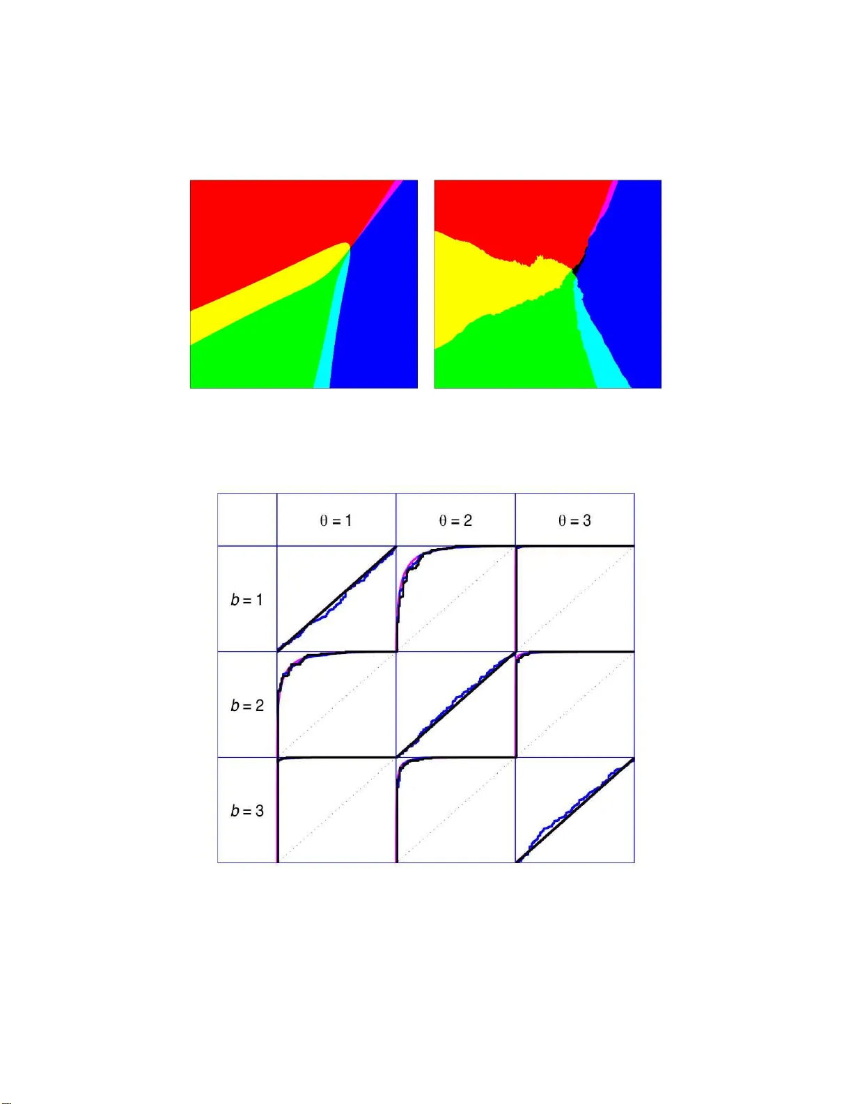
Let $(X,Y)$ be a random variable consisting of an observed feature vector $X\in \mathcal{X}$ and an unobserved class label $Y\in \{1,2,...,L\}$ with unknown joint distribution. In addition, let $\mathcal{D}$ be a training data set consisting of $n$ c…
Authors: Lutz Duembgen, Bernd-Wolfgang Igl, Axel Munk
Electronic Journal of Stat istics V ol. 2 (2008) 468–493 ISSN: 1935-7524 DOI: 10.1214/ 08-EJS24 5 P-v alues for classification Lutz D ¨ um bgen ∗ University of Bern Institute for Mathematic al Statisti cs and A ct uarial Scienc e e-mail: duembgen @stat.un ibe.ch Bernd-W ol fgang Igl † University at L ¨ ub eck Institute of Me dic al Biometry and Statist ics e-mail: bernd.ig l@gmx.de Axel Munk ‡ Ge or gia Au gusta University G¨ ottingen Institute for Mathematic al Sto chastics e-mail: munk@mat h.uni-go ettingen.de Abstract: Let ( X, Y ) b e a random v ariable consisting of an observe d fea- ture v ector X ∈ X and an unobserved class label Y ∈ { 1 , 2 , . . . , L } with un- kno wn joint distribution. In addition, l et D b e a training data set consisting of n completely observ ed indep enden t copies of ( X, Y ). Usual classification procedures provide p oint predictors (classifiers) b Y ( X, D ) of Y or estimate the conditional distribution of Y giv en X . In order to quantify the certain t y of classi f ying X w e propose to construct for each θ = 1 , 2 , . . . , L a p-v alue π θ ( X, D ) for the null h ypothesis that Y = θ , treating Y temp orarily as a fixed parameter. In other words, the p oint predictor b Y ( X, D ) is replaced with a prediction region for Y with a certain confidence. W e argue that (i) this approac h is adv an tag eous ov er traditional approac hes and (ii) an y reasonable classifier can b e mo dified to yield nonparametric p-v alues. W e discuss issues suc h as optimali t y , s i ngle use and multiple use v alidit y , as we ll as computational and graphical asp ects. AMS 2000 sub ject classificat ions: 62C05, 62F25, 62G09, 62G15, 62H30. Keywords and phrases: nearest neighbors, nonparamet ric, optimality, permutation test, prediction region, ROC curve , typica lity index, v alidity. Receiv ed June 2008. 1. In tro duction Let ( X , Y ) b e a random v ar iable consisting of a fea tur e vector X ∈ X and a class lab el Y ∈ Θ := { 1 , . . . , L } with L ≥ 2 poss ible v alues. The jo int distribution of X and Y is determined by the prior probabilities w θ := I P( Y = θ ) and the conditional distributions P θ := L ( X | Y = θ ) for all θ ∈ Θ. Classifying ∗ W ork supported b y Swiss National Science F oundation (SNF) † W ork supported b y German Mi nistry of Education and Research (BMBF) ‡ W ork supported b y German Science F oundation (DFG) 468 L. D ¨ umb gen et al./P-values for c lassific ation 469 such an observ a tion ( X , Y ) mea ns that only X is observed, while Y has to b e predicted somehow. There is a v ast litera ture o n classification, and we refer to McLachlan [ 7 ], Ripley [ 10 ] o r F raley and Raftery [ 4 ] for a n in troduction and further references. Let us assume for the moment that the joint distribution of X and Y is known, so that tra ining data a re no t needed yet. In the simplest cas e, one choo ses a classifier b Y : X → Θ, i.e. a point predictor o f Y . A p ossible extension is to consider b Y : X → { 0 } ∪ Θ, where b Y ( X ) = 0 means that no class is viewed as plausible. A Bay esian appro ach would be to calculate the p o sterior distribution of Y given X , i.e. the poster ior weights w θ ( X ) := I P( Y = θ | X ). In fact, a classifier b Y ∗ satisfying b Y ∗ ( X ) ∈ arg max θ ∈ Θ w θ ( X ) is well-kno wn [ 7 , Cha pter 1] to minimize the r isk R ( b Y ) := I P( b Y ( X ) 6 = Y ) . An obvious adv antage of using the po sterior distribution instead o f the simple classifier b Y ∗ (or b Y ) is additional information ab out confidence. That means, for instance, the p ossibility of co mputing the conditional risk I P ( b Y ∗ ( X ) 6 = Y | X ) = 1 − max θ w θ ( X ). How ever, this dep ends v ery sensitively on the prior weigh ts w θ . Small changes in the latter ma y result in dra stic changes of the po sterior weigh ts w θ ( X ). Mor eov er, if some clas s es θ hav e very small prior weight, the classifier b Y ∗ tends to ig nore these, i. e. the cla ss-dep endent risk I P( b Y ∗ ( X ) 6 = Y | Y = θ ) may b e rather large for some cla sses θ . F o r instance, in medica l applications eac h cla ss ma y correspo nd to a certain disease status while the feature vector co nt ains information ab out patients, including certain symptoms. Here it would b e unacceptable to classify eac h p erso n as being healthy , j ust beca use the diseases in question a r e extremely rare. Note also that some study designs (e.g. case-control studies) allow for the estimation of the P θ but no t the w θ . More over, there ar e applications in which the w θ change o ver time while it is still plausible to ass ume fixed conditional distributions P θ . Another dr awback of the p os ter ior probabilities w θ ( X ) is the following: Sup- po se that the prio r weigh ts w θ are all identical and that for s o me subset Θ o of Θ with at least tw o elements the conditiona l distributions P θ , θ ∈ Θ o , ar e very similar. Then the pos ter ior distribution of Y given X divides the mass corr e - sp o nding to Θ o essentially uniformly amo ng its elements. E ven if the p oint X is right in the ‘cen ter’ of the distributions P θ , θ ∈ Θ o , so that each class in Θ o is per fectly plausible, the po sterior weights ar e no t greater than 1 / #Θ o . If w θ ( X ) is viewed merely as a measur e of plausibilit y of cla ss θ , there is no comp elling reason why these measures should a dd to o ne. T o treat a ll cla s ses impartially , we prop ose to compute for ea ch class θ ∈ Θ a p-v alue π θ ( X ) o f the null hypo thesis that Y = θ . (In this for mu lation we treat Y temp ora rily as an unknown fix e d parameter.) That means, π θ : X → [0 , 1 ] satisfies I P π θ ( X ) ≤ α Y = θ ≤ α for all α ∈ (0 , 1) . (1.1) L. D ¨ umb gen et al./P-values for c lassific ation 470 Given such p-v alues π θ , the set b Y α ( X ) := θ ∈ Θ : π θ ( X ) > α is a (1 − α )–pr ediction region for Y , i.e. I P Y ∈ b Y α ( X ) Y = θ ≥ 1 − α for a rbitrary θ ∈ Θ , α ∈ (0 , 1 ) . If b Y α ( X ) happens to b e a singleton, w e have cla ssified X uniquely with given confidence 1 − α . In ca s e of 2 ≤ # b Y α ( X ) < L w e can a t least exclude some classes with a certain confidence. So far the classifica tio n problem co r resp onds to a simple statistical model with finite parameter space Θ. A distinguishing feature of classification pr ob- lems is that the joint distribution of ( X, Y ) is typically unkno wn and has to be estimated from a set D consisting of completely obs erved training obser- v ations ( X 1 , Y 1 ), ( X 2 , Y 2 ), . . . , ( X n , Y n ). Let us a ssume for the moment that all n + 1 observ ations, i.e. the n training observ ations ( X i , Y i ) and the cur rent observ ation ( X, Y ), are indep endent and iden tically distributed. No w one has to consider c lassifiers b Y ( X , D ) and p-v a lues π θ ( X, D ) dep ending o n the current feature vector X as w ell as on the tra ining data D . In this situation one c a n think of tw o po ssible extensions o f ( 1.1 ): F or any θ ∈ Θ a nd α ∈ (0 , 1), I P π θ ( X, D ) ≤ α Y = θ ≤ α, (1.2) I P π θ ( X, D ) ≤ α Y = θ , D ≤ α + o p (1) as n → ∞ . (1.3) It will turn out that Condition ( 1.2 ) can b e guara n teed in v arious settings. Condition ( 1.3 ) corresp onds to “ mul tiple use” of our p-v alues: Supp ose that w e use the tr aining data D to construct the p-v alues π θ ( · , D ) and clas s ify many future observ a tions ( e X , e Y ). Then the relative n umber o f future observ ations with e Y = b and π θ ( e X , D ) ≤ α is clo se to w b · I P π θ ( X, D ) ≤ α Y = b, D , a random q uantit y dep ending on the training data D . P-v a lues as discussed her e hav e bee n used in s ome sp ecia l cases b efore. F or instance, McLac hlan’s [ 7 ] “t ypicalit y indices” are just p-v alues π θ ( X, D ) sat- isfying ( 1.2 ) in the special ca se of multiv ariate ga ussian distributions P θ ; see also Section 3 . How ev er, McLachl an’s p-v a lues ar e used primarily to identify observ ations no t belo nging to any of the given classes in Θ. In pa r ticular, they are not d esigned and optimized for disti nguishing betw een classes within Θ. Also the use of receiver oper a ting characteristic (R OC) curves in the co ntext of logistic r egressio n or Fisher’s [ 3 ] linear disc riminant a nalysis is related to the present co ncept. One purp os e of this pap er is to provide a so lid foundation for pro cedures of this type. The r emainder o f this pa per is organized as follows: In Section 2 w e r eturn to the idealistic situation of known prior weigh ts w θ and distributions P θ . Here L. D ¨ umb gen et al./P-values for c lassific ation 471 we devise p-v alues that are optimal in a certa in sense and related to the op- timal classifier men tioned prev io usly . These p-v a lues ser ve as a gold standard for p-v alues in realistic settings. In addition we describe briefly McLachlan’s [ 7 ] t ypicality indices and a p otential compromise b etw een the these p-v alues and the optimal ones . Section 3 is devoted to p-v alues inv olving tra ining data. After some general remarks o n cr o ss-v alidation a nd gr aphical repres ent ations, we discuss McL a ch- lan’s [ 7 ] p-v alues in view of ( 1.2 ) a nd ( 1.3 ). Nonparametric p-v alues satisfying ( 1.2 ) without a ny further a ssumptions on the distributions P θ are prop o s ed in Section 3.3 . These p- v alues ar e ba sed on p ermutation testing, and the only pra c- tical res triction is that the group s ize s N θ := # { i : Y i = θ } within the training data should exceed the recipro cal of the in tended test level α . W e claim that any reasona ble classification method can b e conv erted to yield p-v alues. In partic- ular, we introduce p-v alues base d on a suitable v arian t of the nea r est-neighbor method. Section 3.4 deals with asymptotic prop er ties of v ario us p-v a lues as the size n o f D tends to infinit y . It is sho wn in particular that under mild regula r ity conditions the nearest-neigh bo r p-v alues are asy mptotically equiv alent to the optimal metho ds of Section 2 . These results ar e analogous to results o f Stone [ 12 , Section 8] for nea rest-neighbor classifiers . In Section 3.5 the nonparamet- ric p-v alues a re illustrated with simulated a nd real data . Finally , in Section 3.6 we comment on Condition ( 1.3 ) a nd show that the o p (1) cannot b e a voided in general. In Section 4 w e comment briefly on computational as pe c ts o f o ur methods. Section 5 introduces the notion of ‘lo cal identifiabilit y’ for finite mixtures, which is of independent interest. F o r us it is helpf ul to define the optimal p-v a lues in a simple manner and it is also useful fo r the asy mptotic co nsiderations in Section 3.4 . Pro ofs and technical arguments are deferred to Section 6 . Let us mention a differen t t ype o f confidence pro cedure for classification: Suppos e that a θ ( X, D ) , b θ ( X, D ) is a confidence interv al for w θ ( X ). Precisely , let a θ ( X, D ) ≤ w θ ( X ) ≤ b θ ( X, D ) for all θ ∈ Θ with proba bility at least 1 − α . Then ˇ Y ( X , D ) := n θ ∈ Θ : b θ ( X, D ) ≥ ma x η ∈ Θ a η ( X, D ) o would b e a prediction region for Y such that b Y ∗ ( X ) ⊂ ˇ Y ( X , D ) with proba bility at least 1 − α . Note, how ever, that this g ives no control ov er the pr obability that Y 6∈ ˇ Y ( X , D ). In fact, the latter pr o bability could b e clo se to 50 per cent . By wa y of co nt rast, with the p-v alues in the pres ent pap er we can guarantee to cov er Y with a cer tain confidence, even in situations where consis tent estimation of the conditional proba bilities w θ ( X ) is difficult or even impo ssible. 2. Optim al p-v alues and alternativ es Suppos e that the distributions P 1 , . . . , P L hav e known densities f 1 , . . . , f L > 0 with re sp e ct to some measure M on X . Then the marginal distribution o f X L. D ¨ umb gen et al./P-values for c lassific ation 472 has density f := P b ∈ Θ w b f b with resp ect to M , and w θ ( x ) = w θ f θ ( x ) f ( x ) . Hence the optimal classifier b Y ∗ may b e characterized b y b Y ∗ ( X ) ∈ arg max θ ∈ Θ w θ f θ ( X ) . 2.1. Optimal p-v alues Here is an analo g ous consider ation for p-v alues. Let π = ( π θ ) θ ∈ Θ consist of p-v alues π θ satisfying ( 1.1 ). Giv en the latter constraint, our g oal is to provide small p-v a lues a nd small pr e dicio n reg ions. Hence t wo na tural measures of ris k are, for instance, R ( π ) := I E X θ ∈ Θ π θ ( X ) or R α ( π ) := I E # b Y α ( X ) . Elementary ca lculations reveal that R ( π ) = Z 1 0 R α ( π ) dα and R α ( π ) = X θ ∈ Θ R α ( π θ ) with R α ( π θ ) := I P ( π θ ( X ) > α ) . Thu s w e fo cus on minimizing R α ( π θ ) for ar bitrary fixed θ ∈ Θ and α ∈ (0 , 1) under the constraint ( 1.1 ). Since x 7→ 1 { π θ ( x ) > α } may b e viewed as a level– α test o f P θ versus P b ∈ Θ w b P b , a straig ht forward application of the Neyman- Pearson Lemma shows that the p-v alue π ∗ θ ( x ) := P θ z ∈ X : ( f θ /f )( z ) ≤ ( f θ /f )( x ) is optimal, provided that the distribution L ( f θ /f )( X ) is contin uous . Two other repres ent ations of π ∗ θ are given b y π ∗ θ ( x ) = P θ z ∈ X : w θ ( z ) ≤ w θ ( x ) = P θ z ∈ X : T ∗ θ ( z ) ≥ T ∗ θ ( x ) with T ∗ θ := P b 6 = θ w b,θ f b /f θ and w b,θ := w b / P c 6 = θ w c . The fo r mer repr esentation shows that π ∗ θ ( x ) is a non-decrea sing function of w θ ( x ). The la tter represe ntation shows that the prior weight w θ itself is irrelev an t for the optimal p-v alue π ∗ θ ( x ); only the ratios w c /w b with b, c 6 = θ ma tter. In particular, in ca se of L = 2 classes, the optimal p-v alues do not dep end o n the prio r distribution of Y at all. Here and throughout this paper we as sume the likeliho o d ratios T ∗ θ ( X ) to hav e a contin uous distribution. It will be shown in Section 5 that many standar d L. D ¨ umb gen et al./P-values for c lassific ation 473 families of distributions fulfill this condition. In particular, it is satisfied in case of X = R q and P θ = N q ( µ θ , Σ θ ) with parameter s ( µ θ , Σ θ ), Σ θ nonsingular, no t all b eing identical. F urther e x amples include the multiv ariate t -family a s it has been advo cated by Peel and McLachlan [ 8 ] to robustify cluster and discriminant analysis. These authors a lso discuss maxim um lik eliho o d via the EM algo r ithm in this mo del. With out t he contin uit y condition on L ( T ∗ θ ( X )) one c o uld still devise optimal p-v a lues by in tro ducing r andomize d p-v alues , but we refrain from such extensio ns. Let us illustrate the optimal p-v alues in tw o examples inv olving normal dis- tributions: Example 2.1. (Standard mo del) Let P θ = N q ( µ θ , Σ) with mean vectors µ θ ∈ R q and a co mmon symmetric, nons ing ular cov ariance matrix Σ ∈ R q × q . Then T ∗ θ ( x ) = X b 6 = θ w b,θ exp ( x − µ θ ,b ) ⊤ Σ − 1 ( µ b − µ θ ) (2.1) with µ θ ,b := 2 − 1 ( µ θ + µ b ). In the special case of L = 2 classes, let Z ( x ) := ( x − µ 1 , 2 ) ⊤ Σ − 1 ( µ 2 − µ 1 ) / k µ 1 − µ 2 k Σ with the Mahalanobis norm k v k Σ := v ⊤ Σ − 1 v 1 / 2 . Then elementary calculations show that π ∗ 1 ( x ) = Φ − Z ( x ) − k µ 1 − µ 2 k Σ / 2 , π ∗ 2 ( x ) = Φ + Z ( x ) − k µ 1 − µ 2 k Σ / 2 , where Φ denotes the standar d g aussian c.d.f.. In case o f k µ 1 − µ 2 k Σ / 2 ≥ Φ − 1 (1 − α ), b Y α ( x ) = { 1 } if Z ( x ) < −k µ 1 − µ 2 k Σ / 2 + Φ − 1 (1 − α ) , { 2 } if Z ( x ) > + k µ 1 − µ 2 k Σ / 2 − Φ − 1 (1 − α ) , ∅ else . Thu s the tw o classes ar e separated well so that any observ ation X is cla ssified uniquely (o r viewed as suspicious) with confidence 1 − α . In case of k µ 1 − µ 2 k Σ / 2 < Φ − 1 (1 − α ), the feature spa ce contains regions with unique prediction and a reg ion in which bo th class lab els are pla usible: b Y α ( x ) = { 1 } if Z ( x ) ≤ + k µ 1 − µ 2 k Σ / 2 − Φ − 1 (1 − α ) , { 2 } if Z ( x ) ≥ − k µ 1 − µ 2 k Σ / 2 + Φ − 1 (1 − α ) , { 1 , 2 } else . Example 2. 2. Consider L = 3 cla s ses with equal prior weigh ts w θ = 1 / 3 and biv aria te normal distributions P θ = N 2 ( µ θ , Σ θ ), where µ 1 = ( − 1 , 1) ⊤ , µ 2 = ( − 1 , − 1 ) ⊤ , µ 3 = (2 , 0) ⊤ and Σ 1 = Σ 2 = 1 1 / 2 1 / 2 1 , Σ 3 = 0 . 4 0 0 0 . 4 . L. D ¨ umb gen et al./P-values for c lassific ation 474 Fig 1 . P-value functions π ∗ 1 (top left), π ∗ 2 (b ott om left), π ∗ 3 (top right) and a typic al data set (b ott om right) for Example 2.2 . Figure 1 shows a typical sample from this distribution and the cor resp onding p-v alue functions π ∗ θ . The latter ar e on a grey scale with white co rresp onding to zero and black cor resp onding to one. The resulting predition regio ns b Y α ( x ) for α = 5% and α = 1% ar e depicted in Figure 2 . In the latter plots, the color of a p oint x ∈ R 2 has the following meaning: Color b Y α ( x ) Color b Y α ( x ) black ∅ white { 1 , 2 , 3 } red { 1 } yello w { 1 , 2 } green { 2 } cyan { 2 , 3 } dark blue { 3 } magenta { 1 , 3 } (The configura tion b Y α ( x ) = { 1 , 3 } never a ppea red.) Note the influence of α : On the one hand, b Y 0 . 05 ( x ) = ∅ for some x ∈ R 2 but b Y 0 . 05 ( · ) 6 = { 1 , 2 , 3 } in the depicted rectangle. O n the other hand, b Y 0 . 01 ( x ) = { 1 , 2 , 3 } for some x ∈ R 2 while b Y 0 . 01 ( · ) 6 = ∅ . L. D ¨ umb gen et al./P-values for c lassific ation 475 Fig 2 . Pr e dict i on re gions b Y α ( x ) for α = 5% (left) and α = 1% (right) in Example 2.2 . 2.2. T ypic al ity indic es An alternative definition of p-v alues is ba sed on the densities themselv es, namely , τ θ ( x ) := P θ z ∈ X : f θ ( z ) ≤ f θ ( x ) . These typicalit y indices quantif y to what exten t a p oint x is an outlier with resp ect to the single distributions P θ . These p-v alues τ θ are certainly subo ptimal in terms of the r isk R α ( π θ ). On the other hand, they allow for the detection of observ ations which belo ng to none o f the class es under consider ation. Example 2.3. Again let X = R q and P θ = N q ( µ θ , Σ θ ). Since f θ ( X ) is a strictly decreasing function of k X − µ θ k 2 Σ θ with conditional distribution χ 2 q given Y = θ , the typicalit y indices may b e expressed as τ θ ( x ) = 1 − F q k x − µ θ k 2 Σ θ , where F q denotes the c.d.f. o f χ 2 q . These p-v alues allow for the separation of tw o different class es θ , b ∈ Θ only if q − 1 k µ θ − µ b k 2 Σ is sufficiently large. Thus they suffer from the curse of dimensionality and may yield muc h more c o nserv ativ e predition regions than the p-v a lues π ∗ θ . 2.3. Combining the op timal p-values and typic ality indic es The optimal p-v alues π ∗ θ and the typicalit y indices τ θ may b e viewed as extremal mem ber s of a whole family o f p-v alues if we in tro duce an additional class la b el 0 with ‘density’ f 0 ≡ 1 and prior weigh t w 0 > 0. Then we define the co mpromise p-v alue e π θ ( x ) := P θ z ∈ X : ( f θ / e f )( z ) ≤ ( f θ / e f )( x ) L. D ¨ umb gen et al./P-values for c lassific ation 476 with e f := P L b =0 w b f b = f + w 0 . No te that e π θ → τ θ po int wise as w 0 → ∞ , whereas e π θ → π ∗ θ as w 0 → 0 . Example 2.4. In the setting o f Example 2.1 there is a nother mo dification which is similar in spirit to Ehm et a l. [ 1 ]: When defining the p-v alue f or a particular class θ w e replace the other distributions P b = N q ( µ b , Σ), b 6 = θ , with e P b = N q ( µ b , c Σ) for s ome constant c > 1. Thus our mo dified p-v alue b ecomes e π θ ( x ) := P θ z ∈ X : e T θ ( z ) ≥ e T θ ( x ) , where e T θ ( x ) = L X b =1 w b,θ exp k x − µ θ k 2 Σ / 2 − k x − µ b k 2 Σ / (2 c ) = L X b =1 w b,θ exp (1 − c − 1 ) k x − ν θ ,b k 2 Σ / 2 − ( c − 1 ) − 1 k µ b − µ θ k 2 Σ / 2 with ν θ ,b := µ θ − ( c − 1) − 1 ( µ b − µ θ ). 3. T raini ng data Now w e return to the realistic situation of unkno wn distributions P θ and p- v alues π θ ( X, D ) with corres po nding prediction regions b Y α ( X, D ). F rom now on we consider the class labels Y 1 , Y 2 , . . . , Y n as fixed while X 1 , X 2 , . . . , X n and ( X, Y ) are independent with L ( X i ) = P Y i . Tha t way we can cov er the case of i.i.d. training data (via c o nditioning) a s well as s ituations with stratified tra ining samples. In w ha t follows let G θ := i ∈ { 1 , . . . , n } : Y i = θ and N θ := # G θ . W e shall tacitly assume that all g roup sizes N θ are strictly p ositive, and asymp- totic statements as in ( 1.3 ) are meant as n → ∞ and N b /n → w b for all b ∈ Θ . (3.1) 3.1. Visual as sessme nt and estimation of se p ar abi lity Before giving explicit exa mples o f p-v a lues, let us des crib e our wa y of visualizing the separ a bilit y of differen t class e s by mea ns of g iven p-v a lues π θ ( · , · ). F or that purp o se we prop o se to compute cross- v alidated p-v alues π θ ( X i , D i ) for i = 1 , 2 , . . . , n with D i denoting the training data without observ ation ( X i , Y i ). Thus each t raining observ ation ( X i , Y i ) is trea ted tempor arily as a L. D ¨ umb gen et al./P-values for c lassific ation 477 ‘future’ observ a tion to b e class ified with the rema ining data D i . Then we dis- play these cross-v alidated p-v alues gra phically . This is particularly helpful for training samples o f small or mo derate size. In addition to graphica l displays one ca n compute the e mpir ical conditiona l inclusion probabilities b I α ( b, θ ) := # i ∈ G b : θ ∈ b Y α ( X i , D i ) N b and the empirica l pattern pr o babilities b P α ( b, S ) := # i ∈ G b : b Y α ( X i , D i ) = S N b for b, θ ∈ Θ and S ⊂ Θ . These n um bers b I α ( b, θ ) and b P α ( b, S ) can b e in terpreted as estimators of I α ( b, θ | D ) := I P θ ∈ b Y α ( X, D ) Y = b, D and P α ( b, S | D ) := I P b Y α ( X, D ) = S Y = b, D , resp ectively; see also Section 3.4 . F o r larg e gro up sizes N b , one ca n also display the empirica l ROC curv es (0 , 1) ∋ α 7→ 1 − b I α ( b, θ ) which are closely related to the usual R OC curves employ ed, for instance, in logistic reg ression or linear discriminant analysis inv olving L = 2 clas s es. 3.2. T ypic al ity indic es F o r the sa ke of simplicity , supp ose that P θ = N q ( µ θ , Σ) with unkno wn mea n vectors µ 1 , . . . , µ L ∈ R q and an unknown nonsingular cov ariance matrix Σ ∈ R q × q . Consider the standard estimator s b µ θ := N − 1 θ X i ∈G θ X i and b Σ := ( n − L ) − 1 n X i =1 ( X i − b µ Y i )( X i − b µ Y i ) ⊤ . Then the squar ed Mahalanobis distance T θ ( X, D ) := X − b µ θ 2 b Σ can b e used to assess the plausibility of cla ss θ , where we assume that n ≥ L + q . Precisely , C θ := ( n − L − q + 1) q ( n − L )(1 + N − 1 θ ) is a norma lizing constant suc h that C θ T θ ( X, D ) ∼ F q,n − L − q +1 Y = θ ; L. D ¨ umb gen et al./P-values for c lassific ation 478 see [ 7 ]. Here F k,z denotes the F -distribution with k and z degree s of freedo m, and we use the same symbol for the corr esp onding c.d.f.. Hence the typicalit y index τ θ ( X, D ) := 1 − F q,n − L − q +1 ( C θ T θ ( X, D )) is a p-v a lue satisfying ( 1.2 ). Moreov er, s ince the es timato rs b µ b and b Σ a re c o n- sistent , one c a n easily verify prop erty ( 1.3 ) as well. Example 3. 1. An array o f ten electro chemical sensors is used for “smelling” different substances. In each case it pro duces raw data e X ∈ R 10 consisting of the electrica l resis tances of these sensor s . Before analyzing s uch data one should standardize them in order to a chieve in v aria nce with r e s pe ct to the substance’s concentration. O ne po ssible standardiza tion is to repla ce e X with X := e X ( j ) . 10 X k =1 e X ( k ) ! 9 j =1 . Thu s we end up with data vectors in R 9 . F or tec hnical re a sons, group s iz e s N θ are t ypically small, a nd not to o many future observ ations may b e analysed. This is due to the fact that the sy s tem needs to b e recalibr ated regularly . Now we consider a sp ecific da taset with “smells” of L = 12 different brands of tobacc o and fixed gro up sizes N θ = 3 for all θ ∈ Θ. W e c o mputed the cr oss- v alidated t ypicality indices τ θ ( X i , D i ) descr ibe d ab ov e. Figure 3 depicts for each Fig 3 . Cr oss-validate d t ypic ality indic es for tob ac c o “ smel ls”. L. D ¨ umb gen et al./P-values for c lassific ation 479 Fig 4 . 0 . 99 -co nfidenc e pr e dcti on r e gions for tob ac c o “smel ls”. training obser v ation ( X i , Y i ) the p-v alues τ 1 ( X i , D i ) , . . . , τ 12 ( X i , D i ) as a row o f t welv e re c ta ngles. The area of these is pr op ortional to the corresp onding p-v alue. The first three rows co rresp ond to data from the first br and, the next three r ows to the seco nd brand, and so on. Figur e 4 displays the corr esp onding prediction regions b Y α ( X i , D i ) for α = 0 . 01. Within each r ow the elemen ts of b Y α ( X i , D i ) are indicated b y rectangles of full size. These pictures show classes 1 and 2 are separated well from the other eleven classes. Classes 5, 8, 9 and 12 ov erlap somewhat but are clearly sepa rated from the remaining eigh t classes. Finally there are three pair s o f cla sses which a re essentially imp os s ible to distinguish, at least with the present metho d, but whic h are separ ated well fro m the other ten classe s . These pairs ar e 3-4, 6-7, and 1 0-11. It turned out later that brands 6 and 7 were in fact iden tical. Note also that all except o ne prediction region b Y α ( X i , D i ) contain the true class and at most three additional class lab els. 3.3. Nonp ar ametric p-values via p ermutati on tests F o r a particular class θ let I (1) < I (2) < · · · < I ( N θ ) be the elemen ts of G θ . An element ary but useful fact is that ( X, X I (1) , X I (2) , . . . , X I ( N θ ) ) is exchangeable conditional on Y = θ . Thus let T θ ( X, D ) b e a test s ta tistic which is symmetric in ( X I ( j ) ) N θ j =1 . W e define D i ( x ) to be the training da ta with x in place of X i . L. D ¨ umb gen et al./P-values for c lassific ation 480 Then the nonpar ametric p-v alue π θ ( X, D ) := # i ∈ G θ : T θ ( X i , D i ( X )) ≥ T θ ( X, D ) + 1 N θ + 1 (3.2) satisfies requirement ( 1.2 ). Since π θ ≥ ( N θ + 1) − 1 , this pro cedure is useful only if N θ + 1 ≥ α − 1 . In case of α = 0 . 05 this means that N θ should b e at least 1 9 . As fo r the test s tatistic T θ ( X, D ), the optimal p-v alue in Section 2 suggests using a n estimato r fo r the weigh ted likelihoo d ratio T ∗ θ ( x ) or a strictly increas ing transformation thereof. In very high-dimensiona l settings this may b e too am- bitious, and T θ ( X, D ) could b e a ny test statistic quantifying the implausibility of “ Y = θ ” . Plug-in statistic for standard gaussian m o del . F or the setting of E xam- ple 2.1 a nd Sec tio n 3.2 o ne could replace the unknown pa r ameters w c , µ c and Σ in T ∗ θ with N c /n , b µ c and b Σ, r esp ectively . Note that the resulting p -v alues alwa ys satisfy ( 1.2 ), even if the underlying distributions P c are not gaussian with common cov ar iance matrix. Nearest-neighbor estimation. One could estimate w θ ( · ) via nearest neigh- bo rs. Supp ose that d ( · , · ) is some metric on X . Let B ( x, r ) := { y ∈ X : d ( x, y ) ≤ r } , and for a fixed po sitive integer k ≤ n define b r k ( x ) = b r k ( x, D ) := min r ≥ 0 : # { i ≤ n : X i ∈ B ( x, r ) } ≥ k . F ur ther let b P θ denote the empirica l distribution of the p oints X i , i ∈ G θ , i.e. b P θ ( B ) := N − 1 θ # { i ∈ G θ : X i ∈ B } for B ⊂ X . Then the k -nea rest-neighbor estimator o f w θ ( x ) is given by b w θ ( x, D ) := b w θ b P θ B ( x, b r k ( x )) . X b ∈ Θ b w b b P b B ( x, b r k ( x )) with certain estimators b w b = b w b ( D ) of w b . The resulting nonpara metric p-v alue is defin ed wit h T θ ( x, D ) := − b w θ ( x, D ). Note that in cas e of b w b = N b /n , we simply end up with the r atio b w θ ( x, D ) = # i ∈ G θ : d ( X i , x ) ≤ b r k ( x ) . # i ≤ n : d ( X i , x ) ≤ b r k ( x ) . F o r simplicit y , we ass ume k to b e determined by the gr oup sizes N 1 , . . . , N L only . Of course one could define π θ ( X, D ) with k = k θ ( X, D ) nearest neig h bo rs of X , as long a s k θ ( X, D ) is sy mmetric in the N θ + 1 featur e v ectors X and X i , i ∈ G θ . Moreover, in applications where the different co mpo nent s of X ar e measured o n rather different scales, it might be rea s onable to replace d ( · , · ) with some data-dr iven metric. L. D ¨ umb gen et al./P-values for c lassific ation 481 Logistic regression. Suppo se for simplicity that there are L = 2 classes and that X ∈ R d contains the v alues of d num erical or binary v ar ia bles. Let ( b a, b b ) = ( b a ( D ) , b b ( D )) b e the maximum lik elihoo d estimato r for the pa rameter ( a, b ) ∈ R × R d in the lo gistic mo del, where log w 2 ( x ) 1 − w 2 ( x ) = a + b ⊤ x. Then p ossible ca ndidates for T 1 ( x, D ) a nd T 2 ( x, D ) a re given b y T 1 ( x, D ) := b a + b b ⊤ x =: − T 2 ( x, D ) . Extensions to multicategory log is tic regress ion as well a s the inclusion of regu- larization terms to deal with high-dimensional cov ariable vectors X a re p oss ible and will b e describ ed elsewhere . 3.4. Asymptotic pr op erties Now we analyze the asymptotic b ehavior of the nonparametric p-v alues π θ ( X, D ) and the co rresp onding empirical probabilities b I α ( b, θ ) and b P ( b, S ). Throughout this section, a symptotic statements a re to b e understo o d within setting ( 3.1 ). As in Sectio n 2 w e a ssume that the distributions P θ hav e strictly p ositive densities with respe ct to s ome mea sure M on X . The following theorem implies that π θ ( X, D ) sa tisfies ( 1.3 ) under certain conditions on the underlying test statistic T θ ( X, D ). In addition the empirical probabilities b I α ( b, θ ) a nd b P ( b, S ) turn o ut to b e c o nsistent estimato r s of I α ( b, θ | D ) and P α ( b, S | D ), resp ectively . Theorem 3.1. Supp ose that for fixe d θ ∈ Θ ther e exists a test statistic T o θ on X satisfying the fol lowing t wo r e quir ements: T θ ( X, D ) → p T o θ ( X ) , (3.3) L ( T o θ ( X )) is c ontinuous . (3.4) Then π θ ( X, D ) → p π o θ ( X ) , (3.5) wher e π o θ ( x ) := P θ z ∈ X : T o θ ( z ) ≥ T o θ ( x ) . In p articular, for arbitr ary fixe d α ∈ (0 , 1) , R α ( π θ ( · , D )) → p R α ( π o θ ) , (3.6) I α ( b, θ | D ) b I α ( b, θ ) ) → p I P( π o θ ( X ) > α | Y = b ) for e ach b ∈ Θ . (3.7) L. D ¨ umb gen et al./P-values for c lassific ation 482 If the limiting test s tatistic T o θ is equal to T ∗ θ or so me strictly incr e a sing tra ns - formation thereof, then the nonparametric p-v alue π θ ( · , D ) is asymptotically optimal. The nex t tw o lemmata describe situations in which Condition ( 3.3 ) or ( 3.4 ) is s atisfied. Lemma 3.2. C onditions ( 3.3 ) and ( 3.4 ) ar e satisfie d in c ase of t he plug-in rule for the homosc e dastic gaussian mo del, pr ovide d that I E( k X k 2 ) < ∞ and L ( X ) has a L eb esgue density. Lemma 3.3. Supp ose t hat ( X , d ) is a sep ar able met ric sp ac e and that al l densi- ties f b , b ∈ Θ , ar e c ontinuous on X . Al ternatively, su pp ose that X = R q e quipp e d with some n orm. Then Condition ( 3.3 ) is satisfie d with T o θ = T ∗ θ in c ase of the k -ne ar est-neighb or rule with b w θ = N θ /n , pr ovide d that k = k ( n ) → ∞ and k /n → 0 . 3.5. Examples The nonparametric p-v alues are illustrated with tw o examples. Example 3.2. The low er right pa nel in Figure 1 shows simulated tra ining data from the mo del in Example 2 .2 , where N 1 = N 2 = N 3 = 100. Now we co mputed the corr esp onding prediction regions b Y 0 . 05 ( x, D ) ba s ed on the plug-in metho d for the standard g aussian mo del (which isn’t correct here) a nd on the nearest- neighbor metho d with k = 10 0 and standar d euclidea n distance. Figure 5 depicts these prediction r egions. T o judge the p erfor ma nce of the nonpar ametric p-v a lues visually w e chose R OC curves, where we concent rated on the plug-in metho d. In Figure 6 we show for each pair ( b, θ ) ∈ Θ × Θ the true ROC curv es of π ∗ θ ( · ) and π θ ( · , D ), (0 , 1) ∋ α 7→ ( I P π ∗ θ ( X ) ≤ α Y = b (magenta ) , I P π θ ( X, D ) ≤ α Y = b, D = 1 − I α ( b, θ | D ) (blue) , bo th of which had b een estimated in 40’000 Mo nt e Ca rlo Simulations o f X ∼ P θ . In addition we sho w the empirical R O C curv e α 7→ 1 − b I α ( b, θ ) (blac k step function). Note first that the difference b etw een the (conditional) R OC curve of π θ ( · , D ) and its empirica l counterpart 1 − I α ( b, θ | D ) is a lwa ys r ather small, despite the mo der ate group sizes N b = 100 . Note further that the R OC curves of π θ ( · , D ) and π ∗ θ ( · ) are als o close together, despite the fact that the plug- in method uses a n incorr ect mo del. These pictures show clea rly that distinguishing betw een class e s 1 and 2 is mo r e difficult than distinguishing betw een classes 2 and 3, while classes 1 and 3 ar e separa ted almost per fectly . Of co ur se these pictures give o nly partial information a bo ut the p erforma nce of the p-v alues. In a ddition one co uld inv estigate the joint distribution of the p-v alues via pattern pro ba bilities; see also the next example. L. D ¨ umb gen et al./P-values for c lassific ation 483 Fig 5 . Pr e diction r e gions b Y 0 . 05 ( x, D ) with plug-in metho d (left) and ne ar est neighb or metho d (right) for Example 3.2 . Fig 6 . ROC curve s for the plug-in metho d applie d to the data in Example 3.2 . L. D ¨ umb gen et al./P-values for c lassific ation 484 T able 1 Empiric al p erforma nc e of b Y 0 . 05 ( · , · ) and b Y 0 . 01 ( · , · ) in Example 3.3 . b Y 0 . 05 ( X i , D i ) b Y 0 . 01 ( X i , D i ) Y i ∋ 1 ∋ 2 = { 1 } = { 2 } = { 1 , 2 } ∋ 1 ∋ 2 = { 1 } = { 2 } = { 1 , 2 } 1 .950 .244 . 756 .050 .194 .990 .448 . 552 .010 .438 .950 .222 . 778 .050 .172 .990 .452 . 548 .010 .443 .952 .233 . 767 .048 .185 .990 .449 . 551 .010 .440 2 .396 .950 . 050 .604 .346 .743 .991 . 009 .257 .734 .356 .950 . 050 .644 .307 .698 .991 . 009 .302 .689 .406 .950 . 050 .594 .356 .773 .992 . 008 .227 .766 Example 3. 3. This example is fro m a data base o n quality management at the Univ ersit y hospital at L¨ ub eck. In a longterm study on mortality of pa tien ts after a cer ta in type of heart surg ery , data of mor e than 20 ’000 cases hav e bee n rep orted. The dep endent v ariable is Y ∈ { 1 , 2 } with Y = 1 and Y = 2 meaning that the patient survived the o p eration or no t, resp ectively . F or each cas e there were q = 21 nu merical or binary cov ar iables des cribing the patient (e.g. sex, age, v a rious sp ecific risk factors) plus cov ariables desc r ibing the circumstances of the op er a tion (e.g. emerge ncy or not, ex per ience of the surgeo n). W e reduced the data set by ta k ing all N 1 = 662 observ ations with Y = 2 and a random subsa mple of N 1 = 3 N 2 = 1986 observ ations with Y = 1. Without such a r e duction, the nearest-neighbor metho d wouldn’t work well due to the very different gro up siz e s . Now w e computed no npa rametric cro ssv a lida ted p- v alues ba sed on the plug-in metho d from the standard g aussian mo del, lo g istic regress io n, and the nearest-neighbor metho d with k = 200. In the la tter case, we first divided each comp onent of X cor resp onding to a no n-dichotomous v ar ia ble b y its sample standard deviation, b ecause the v aria bles are measured on v ery different sca les. T able 1 r ep orts the p erformance of b Y α ( X i , D i ) as a predictor of Y i for α = 5% and α = 1%. In each cell of the table the e ntries cor resp ond to the three metho ds men tioned ab ov e. This ex a mple shows the p-v alues’ p otential to cla ssify a certain fraction o f cases unambiguously even in s ituations in which ov erall risks o f class ifier s ar e not small w hich is rather typ ical in medical ap- plications. Note a g ain that the metho d doesn’t require a ny knowledge of prio r probabilities. Lo gistic r egressio n yielded s lightly b e tter results than the other t wo in terms of the fraction of cases with b Y α ( X i , D i ) = { Y i } . The other tw o methods p erformed similarly . 3.6. Im p ossibility of str engthening ( 1.3 ) Comparing ( 1.2 ) and ( 1.3 ), one might w ant to strengthen the la tter requirement to I P π θ ( X, D ) ≤ α Y = θ , D ≤ α almost s urely . (3.8) How ev er, the following lemma entails that there are no reaso nable p-v alues satisfying ( 3.8 ). Recall that we a re aiming at p-v alues such that I P π θ ( X, D ) ≤ α Y = b is lar ge for b 6 = θ . L. D ¨ umb gen et al./P-values for c lassific ation 485 Lemma 3.4. L et Q 1 , Q 2 , . . . , Q L b e mutual ly absolutely c ont inu ous pr ob ability distributions on X . S upp ose that ( 3.8 ) is satisfie d whenever ( P 1 , P 2 , . . . , P L ) is a p ermu tation of ( Q 1 , Q 2 , . . . , Q L ) . In that c ase, for arbitr ary b ∈ Θ , I P π θ ( X, D ) ≤ α Y = b, D ≤ α almost s u r ely . 4. Computational asp ects The computation of the p-v alues in ( 3.2 ) may b e rather time-consuming, de- pending on the particular test statistic T θ ( · , D ). Just think ab out classification methods in v olving v aria ble s election or tuning of ar tificial neural netw orks by means of D . Also the nearest-neighbor method wit h some data - driven choice of k or the metric d ( · , · ) ma y result in tedious procedures. In o rder t o com- pute π θ ( · , D ) as well as π θ ( X i , D i ) one can typically reduce the computational complexity co nsiderably by using suitable up date fo r mulae or s hortcuts. Naiv e shortcuts for the nonparametric p-v al ue s. One might be tempted to replace π θ ( X, D ) with the naive p-v alues π naive θ ( X, D ) := # i ∈ G θ : T θ ( X i , D ) ≥ T θ ( X, D ) + 1 N θ + 1 . (4.1) One can easily show that the conclusions o f Theorem 3.1 r emain true with π naive θ ( · , · ) in place of π θ ( · , · ). How ever, finite sample v alidity in the sense of ( 1.2 ) is not satisfied in general, s o we prefer the alter na tive shortcut des crib ed next. No te also that empirical ROC curves offered by s ome sta tistical so ft w are pack ages, as a co mplemen t to logistic reg ression or linear discriminant a nalysis with tw o classes, are often bas ed on this shortcut. V alid shortcuts for the nonparametric p-v alues. Often the computa- tions as well as the progr a m code b ecome muc h simpler if we re pla ce T θ ( X, D ) and T θ ( X i , D i ( X )) in Definition ( 3.2 ) with T θ ( X, D ( X , θ )) and T θ ( X i , D ( X , θ )), resp ectively , where D ( X , θ ) denotes the training data D a fter adding the “obser- v ation” ( X , θ ). That means, b efore judging whether θ is a plausible class lab el for a new o bs erv a tio n X , we augmen t the tr a ining data by ( X, θ ) to determine the test statistic T θ ( · , D ( X , θ )). Then we just ev aluate the latter function at the N θ + 1 p oints X and X i , i ∈ G θ , to co mpute π naive θ ( X, D ( X , θ )) = # i ∈ G θ : T θ ( X i , D ( X , θ )) ≥ T θ ( X, D ( X , θ )) + 1 N θ + 1 . This p-v alue do es satisfy Condition ( 1.2 ), and the co nclus io ns of Theorem 3.1 remain true as well. In this context it migh t b e helpful if the underlying test statistics satisfy s o me mo derate robustness prop erties, beca use X may be an outlier with r e s pe c t to the distribution P θ . L. D ¨ umb gen et al./P-values for c lassific ation 486 Up date formulae for sample means and co v ariances. In co nnection with the typicalit y indices of Section 3.2 or the plug-in metho d for the s tandard gaussian model, elementary calculations reveal the following up date formulae for g roupwise mean vectors a nd sa mple cov aria nce matrices: Replacing D with the reduced data set D i for some i ∈ G θ has no impact on b µ b for b 6 = θ while b Σ ← ( n − L − 1) − 1 ( n − L ) b Σ − (1 − N − 1 θ ) − 1 ( X i − b µ θ )( X i − b µ θ ) ⊤ , b µ θ ← ( N θ − 1) − 1 ( N θ b µ θ − X i ) = b µ θ − ( N θ − 1) − 1 ( X i − b µ θ ) . Replacing D with the mo dified data set D i ( X ) for s o me i ∈ G θ results in b Σ ← ( n − L ) − 1 ( n − L ) b Σ + (1 − N − 1 θ ) ( X − b µ θ ,i )( X − b µ θ ,i ) ⊤ − ( X i − b µ θ ,i )( X i − b µ θ ,i ) ⊤ , b µ θ ← b µ θ + N − 1 θ ( X − X i ) , where b µ θ ,i := ( N θ − 1) − 1 ( N θ b µ θ − X i ). Finally , re pla cing D with the augmented data set D ( X , θ ) means that b Σ ← ( n + 1 − L ) − 1 ( n − L ) b Σ + (1 + N − 1 θ ) − 1 ( X − b µ θ )( X − b µ θ ) ⊤ , b µ θ ← ( N θ + 1) − 1 N θ b µ θ + X = b µ θ + ( N θ + 1) − 1 ( X − b µ θ ) . Up date formulae for the nearest-nei gh b or m etho d. F or conv enience we restr ict our a tten tion to the v alid s hortcut inv olving D ( X , θ ). T o compute the r esulting p-v alues b π naive θ ( X, D ( X , θ )) quic kly for arbitrary feature v ectors X ∈ X , it is co nv enien t to store the n (1 + 2 L ) num bers b r k ( X i , D ) , N k − 1 ,b ( X i , D ) , N k,b ( X i , D ) with i ∈ { 1 , . . . , n } and b ∈ Θ , where N ℓ,b ( x, D ) := # i ∈ { 1 , . . . , n } : Y i = b, d ( x, X i ) ≤ b r ℓ ( x, D ) . F o r then o ne can easily verify that N k,b ( X i , D ( X , θ )) = N k − 1 ,b ( X i , D ) + 1 { b = θ } if d ( X i , X ) < b r k ( X i , D ) N k,b ( X i , D ) + 1 { b = θ } if d ( X i , X ) = b r k ( X i , D ) , N k,b ( X i , D ) if d ( X i , X ) > b r k ( X i , D ) . Hence classifying a new feature vector X requires only O ( n ) steps for deter- mining the 1 + L 2 n um be r s b r k ( X, D ( X , θ )) and N b ( X, D ( X , θ )) and t he nL 2 n um be r s N b ( X i , D ( X , θ )), where 1 ≤ i ≤ n and b, θ ∈ Θ. Computing the cros s v alidated p-v alues with the v alid shortcut is particular ly easy , b ecause replacing one training observ ation ( X i , Y i ) with ( X i , θ ) do es not affect the ra dii b r k ( x, D ). In case o f data-dr iven choice o f k or d ( · , · ), the preceding fo r mulae ar e no longer applicable. Then the v alid shortcut is particularly useful to reduce the computational complexity . L. D ¨ umb gen et al./P-values for c lassific ation 487 5. Lik eliho o d ratios and l o cal iden tifiability In previous sections we ass umed that the distribution o f likelihoo d r atios such as w θ ( X ) or T ∗ θ ( X ) is co nt in uous. This prop erty is related to a pro p erty which we call ‘lo cal ident ifiabilit y’, a stre ng thening o f the well-kno wn notion of identifiabil- it y for finite mixtures. Throughout this section we assume that the distributions P 1 , P 2 , . . . , P L belo ng to a given mo del ( Q ξ ) ξ ∈ Ξ of pro babilit y distributions Q ξ with densities g ξ > 0 with res pe c t to some measure M on X . Iden tifiabilit y . Let us first recall Y ako witz and Spr a gins’ [ 13 ] definition of iden tifiabilit y fo r finite mixture s . Th e f amily ( Q ξ ) ξ ∈ Ξ is called identifiable , if the following condition is satisfied: F or ar bitrary m ∈ N let ξ (1 ) , . . . , ξ ( m ) be pairwise different parameters in Ξ and let λ 1 , . . . , λ m > 0. If ξ ′ (1) , . . . , ξ ′ ( m ) ∈ Ξ and λ ′ 1 , . . . , λ ′ m ≥ 0 such that m X j =1 λ j Q ξ ( j ) = m X j =1 λ ′ j Q ξ ′ ( j ) , then ther e exists a permutation σ of { 1 , 2 , . . . , m } such that ξ ′ ( i ) = ξ ( σ ( i )) and λ ′ i = λ σ ( i ) for i = 1 , 2 , . . . , m . Evidently the family ( Q ξ ) ξ ∈ Ξ is identifiable if the density functions g ξ , ξ ∈ Ξ, are linearly independent as elemen ts of L 1 ( M ), and the con verse statement is also true [ 13 ]. A standard ex a mple of an iden tifiable family is the s e t o f all nondegenerate gaussian distributions o n R q ; see [ 13 ]. Holzmann et a l. [ 6 ] provide a r ather com- prehensive list of ident ifiable cla s ses of multiv ariate distributions. In particular, they verify identi fiability of families of elliptically symmetric distributions o n X = R q with Leb esgue densities of the form g ξ ( x ) = det(Σ) − 1 / 2 h q ( x − µ ) ⊤ Σ − 1 ( x − µ ); ζ . (5.1) Here the parameter ξ = ( µ, Σ , ζ ) consists of an arbitrary lo cation parameter µ ∈ R q , an arbitra ry symmetric and p ositive definite scatter ma tr ix Σ ∈ R q × q and a n additional shap e para meter ζ which may also v a ry in the mixture . F o r each shap e parameter ζ , the ‘densit y ge ner ator’ h q ( · ; ζ ) is a nonnegativ e function on [0 , ∞ ) such that R X h q ( k x k 2 ; ζ ) dx = 1. O ne particular exa mple are the multiv ariate t –distributions with h q ( u ; ζ ) = Γ(( ζ + q ) / 2) π q/ 2 Γ( ζ / 2) (1 + u ) − ( ζ + q ) / 2 for ζ > 0. W e men tion that the subsequen t arguments apply to most of the elliptically symmetric families discussed by Holzmann et al. [ 6 ]. Peel et a l. [ 9 ] discuss cla s sification for directional data a nd our metho d can be extended to distributions with non-euclidean domain, combining the arguments below with methods in Ho lzma nn et al. [ 5 ]. As prominent exa mples we mention the von Mises family for directional data and the K ent family for spherical da ta. L. D ¨ umb gen et al./P-values for c lassific ation 488 Con tin uit y of l i k eliho o d ratios. Suppo se that P θ = Q ξ ( θ ) with pa rameters ξ (1), . . . , ξ ( L ) in Ξ which are not all identical. Then one can easily verify that contin uity of L ( w θ ( X )) or L ( T ∗ θ ( X )) follows from the following condition: The family ( Q ξ ) ξ ∈ Ξ is called lo c ally identifiable , if for ar bitrary m ∈ N , pairwise different para meters ξ (1) , . . . , ξ ( m ) ∈ Ξ a nd num bers β 1 , . . . , β m ∈ R , M ( x ∈ X : m X j =1 β j g ξ ( j ) ( x ) = 0 ) > 0 implies that β 1 = β 2 = · · · = β m = 0 . Lo cal iden tifiabilit y entails the follo wing conclusion: Suppose that Q is equal to P m j =1 λ j Q ξ ( j ) for so me num ber m ∈ N , pair wis e different parameters ξ (1), . . . , ξ ( m ) in Ξ and no nneg ative n um ber s λ 1 , . . . , λ m . Then one can determine the ingr edients m , ξ (1) , . . . , ξ ( m ) a nd λ 1 , . . . , λ m from the restr iction of Q to any fixed measurable set B o ⊂ X with M ( B o ) > 0 . The following theorem provides a sufficien t criterion for lo ca l iden tifiabilit y whic h is easily verified in many s ta ndard examples. Theorem 5. 1. L et M b e L eb esgue me asur e on X = X 1 × X 2 × · · · × X q with op en intervals X k ⊂ R . Supp ose that the fol lowing two c ondi tions ar e satisfie d: (i) ( Q ξ ) ξ ∈ Ξ is identifiable; (ii) for arbitr ary ξ ∈ Ξ , k ∈ { 1 , 2 , . . . , q } and x i ∈ X i , i 6 = k , the function t 7→ g ξ ( x 1 , . . . , x k − 1 , t, x k +1 , . . . , x q ) may b e extende d to a holomorp hic function on some op en subset of C c ontaini ng X k . Then the family ( Q ξ ) ξ ∈ Ξ is lo c al ly identifiable. One can easily verify that Condition (ii) of Theorem 5.1 is satisfied by the densities g ξ in ( 5.1 ), if the density g enerators h q ( · ; ζ ) may b e extended to ho lo- morphic functions on some op en subset of C containing [0 , ∞ ). Hence, for in- stance, the family of all multiv ariate t –distributions is lo ca lly identifi able. 6. Pro ofs Pr o of of The or em 3.1 . Since the distributions P 1 , . . . , P L are mutually abso- lutely contin uous, Condition ( 3.3 ) entails that ρ ( ǫ, N 1 , . . . , N L ) := max a,b ∈ Θ; i =1 ,...,n Z I P | T θ ( x, D i ( z )) − T o θ ( x ) | ≥ ǫ P a ( dx ) P b ( dz ) tends to zer o for a ny fixed ǫ > 0. It follows from the elementary inequality 1 { r ≥ s } − 1 { r o ≥ s o } ≤ 1 {| r − r o | ≥ ǫ } + 1 {| s − s o | ≥ ǫ } + 1 {| r o − s o | < 2 ǫ } L. D ¨ umb gen et al./P-values for c lassific ation 489 for real num bers r, r o , s, s o that π θ ( X, D ) = ( N θ + 1) − 1 1 + X i ∈G θ 1 T θ ( X i , D i ( X )) ≥ T θ ( X, D ) ! = N − 1 θ X i ∈G θ 1 T θ ( X i , D i ( X )) ≥ T θ ( X, D ) + R 1 = N − 1 θ X i ∈G θ 1 T o θ ( X i ) ≥ T o θ ( X ) + R 1 + R 2 ( ǫ ) , where | R 1 | ≤ ( N θ + 1) − 1 and | R 2 ( ǫ ) | ≤ N − 1 θ # n i ∈ G θ : T θ ( X i , D i ( X )) − T o θ ( X i ) ≥ ǫ o + 1 n T θ ( X, D ) − T o X ( X ) ≥ ǫ o + N − 1 θ # n i ∈ G θ : T o θ ( X i ) − T o θ ( X ) < 2 ǫ o . Hence I E | R 2 ( ǫ ) | ≤ 2 ρ ( ǫ, N 1 , . . . , N L ) + ω (2 ǫ ) → ω (2 ǫ ), where ω ( δ ) := sup r ∈ R P θ z ∈ X : | T o θ ( z ) − r | < δ ↓ 0 ( δ ↓ 0) b y virtue of Condition ( 3.4 ). These considerations show that π θ ( X, D ) = b F θ ( T o θ ( X )) + o p (1) = F θ ( T o θ ( X )) + o p (1) , where F θ ( r ) := P θ z ∈ X : T o θ ( z ) ≥ r , b F θ ( r ) := b P θ z ∈ X : T o θ ( z ) ≥ r . Here we utilized the w ell-known fact [ 11 ] that k b F θ − F θ k ∞ = o p (1). Since π o θ ( X ) = F θ ( T o θ ( X )), this entails Conclusion ( 3.5 ). As to the rema ining assertions ( 3.6 – 3.7 ), note fir st that ( 3.5 ) implies that τ ( ǫ, N 1 , . . . , N L ) := max a,b ∈ Θ; i =1 ,...,n Z I P | π θ ( x, D i ( z )) − π o θ ( x ) | ≥ ǫ P a ( dx ) P b ( dz ) tends to zer o for a ny fixed ǫ > 0, again a co nsequence of mu tual a bsolute contin uity of P 1 , . . . , P L . Similarly a s in the pro of o f ( 3.5 ) one ca n verify that I α ( b, θ | D ) = I P( π θ ( X, D ) > α | Y = b, D ) = G b,θ ( α ) + R ( ǫ ) , b I α ( b, θ ) = N − 1 b X i ∈G b 1 π θ ( X i , D i ) > α = b G b,θ ( α ) + b R ( ǫ ) = G b,θ ( α ) + b R ( ǫ ) + o p (1) , L. D ¨ umb gen et al./P-values for c lassific ation 490 with G b,θ ( u ) := P b z ∈ X : π o θ ( z ) > u and b G b,θ ( u ) := b P b z ∈ X : π o θ ( z ) > u , while I E | R ( ǫ ) | ≤ τ ( ǫ, N 1 , . . . , N L ) + I P | π o θ ( X ) − α | < ǫ Y = b → I P | π o θ ( X ) − α | < ǫ Y = b , I E | b R ( ǫ ) | ≤ τ ( ǫ, N 1 , . . . , N b − 1 , N b − 1 , N b +1 , . . . , N L ) + I P | π o θ ( X ) − α | < ǫ Y = b → I P | π o θ ( X ) − α | < ǫ Y = b . Since the latter probability tends to zero as ǫ ↓ 0, we obtain Claim ( 3.7 ). This implies Claim ( 3.6 ), bec a use R α ( π θ ( · , D )) = X b ∈ Θ w b I α ( b, θ | D ) → p X b ∈ Θ w b I P( π o θ ( X ) > α | Y = b ) = R α ( π o θ ) . ✷ Pr o of of L emma 3.2 . It is a simple co nsequence of the weak law o f large n um- ber s that b µ b → p µ b := I E ( X | Y = b ) and b Σ → p Σ := P L b =1 w b V a r( X | Y = b ). Now one can easily show that ( 3.3 ) is satisfied with T o θ defined as in ( 2.1 ). The results fro m Section 5 ent ail that Leb q x ∈ R q : T o θ ( x ) = c = 0 for any c > 0, so that ( 3.4 ) is satisfied as well. ✷ Pr o of of L emma 3.3 . The assumptions imply the existence of a Borel set X o ⊂ X with I P( X ∈ X o ) = 1 such that the following additional r equirements ar e satisfied: I P( X ∈ B ( x, r )) > 0 for all x ∈ X o , r > 0 , (6.1) lim r ↓ 0 P b ( B ( x, r )) P θ ( B ( x, r )) = f b f θ ( x ) for all θ , b ∈ Θ , x ∈ X o . (6.2) In ca se o f co nt in uous densities f 1 , f 2 , . . . , f L > 0 o n a separa ble metric space ( X , d ), this is easily verified with X o being the supp ort of L ( X ), i.e. the smallest closed s et such that I P ( X ∈ X o ) = 1. In case o f X = R q and d ( x, y ) = k x − y k , existence of such a set X o is a known result from geometric measure theory; cf. F e der er [ 2 , Theorem 2 .9.8]. In view of ( 6.1 – 6.2 ), it suffices to show that for ar bitrary fixed x ∈ X o and b ∈ Θ, b r k ( n ) ( x ) → p 0 and b P b B ( x, b r k ( n ) ( x )) P b B ( x, b r k ( n ) ( x )) → p 1 . (6.3) T o this end, note first that the r andom n um ber s N ( x, r ) := # { i : d ( X i , x ) < r } L. D ¨ umb gen et al./P-values for c lassific ation 491 satisfy I E N ( x, r ) = X θ ∈ Θ N θ P θ { z : d ( z , x ) < r } = n I P( d ( X , x ) < r ) + o (1) uniformly in r ≥ 0 , (6.4) V a r( N ( x, r )) = X θ ∈ Θ N θ P θ { z : d ( z , x ) < r } 1 − P θ { z : d ( z , x ) < r } ≤ min I E N ( x, r ) , n / 4 . (6.5) If we define r n := max r ≥ 0 : I E N ( x, r ) ≤ k ( n ) / 2 , then I P b r k ( n ) ( x ) < r n = I P N ( x, r n ) ≥ k ( n ) ≤ I P N ( x, r n ) − I E N ( x, r n ) ≥ k ( n ) / 2 ≤ I E N ( x, r n ) / ( k ( n ) / 2) 2 ≤ 2 /k ( n ) → 0 b y Tshebyshev’s ineq ua lit y and ( 6.5 ). On the other ha nd, for any fixed ǫ > 0 , I P b r k ( n ) ( x ) ≥ ǫ = I P N ( x, ǫ ) < k ( n ) = I P N ( x, ǫ ) − I E N ( x, ǫ ) ≤ n o (1) − I P( d ( X , x ) < ǫ ) = O (1 /n ) according to ( 6.4 ) and ( 6.1 ). These considerations show that b r k ( n ) ( x ) → p 0, but b r k ( n ) ( x ) ≥ r n with asymptotic pro bability one. Now we utilize that the pro cess r 7→ b P b ( B ( x, r )) P b ( B ( x, r )) − 1 is a zero mean r e verse mar tingale on r ≥ 0 : I P ( d ( X , x ) ≤ r ) > 0 ⊃ (0 , ∞ ), so that Do ob’s inequa lit y entails that I E s up r ≥ r n b P b ( B ( x, r )) P b ( B ( x, r )) − 1 2 ≤ 4 N b P b ( B ( x, r n )) = O ( k ( n ) − 1 ); see Shora ck and W ellner [ 11 , Sections 3.6 and A.10 -11]. The latter considera tions imply the s econd part of ( 6.3 ). ✷ Pr o of of The or em 5.1 . The pro of is by contradiction. T o this end supp os e that there ar e m ≥ 2 pa irwise different parameters ξ (1) , ξ (2) , . . . , ξ ( m ) ∈ Ξ and nonzero real num ber s β 1 , β 2 , . . . , β m such that h := P m i =1 β i g ξ ( i ) satisfies Leb q ( W ) > 0 with W := { x ∈ X : h ( x ) = 0 } . In case of q = 1, this entails that W ⊂ X = X 1 contains a n accumultation po int within X 1 , and the iden tit y theorem fo r analytic functions yields that h = 0 o n X . But this would be a contradiction to ( Q ξ ) ξ ∈ Ξ being identifiable. L. D ¨ umb gen et al./P-values for c lassific ation 492 In case of q > 1 , by F ubini’s theorem, Leb q ( W ) = Z X 1 ×···×X q − 1 Leb 1 { t : ( x ′ , t ) ∈ W } Leb q − 1 ( dx ′ ) > 0 , whence Leb 1 { t : ( x ′ , t ) ∈ W } > 0 for all x ′ in a measurable set W ′ ⊂ X 1 × · · · × X q − 1 such that Leb q − 1 ( W ′ ) > 0. Hence the identit y theorem for ana lytic functions, applied to t 7→ h ( x ′ , t ) implies that W ′ × X q ⊂ W. Since Leb q − 1 ( W ′ ) > 0, we may pro ceed inductively , consider ing for k = q − 1 , q − 2 , . . . , 1 the functions t 7→ h ( x ′′ , t, x k +1 , . . . , x q ) on X k . Even tually we obtain W = X , but this would b e a contradiction to ( Q ξ ) ξ ∈ Ξ being identifi able. ✷ Pr o of of L emma 3.4 . F or any per mu tation σ o f (1 , 2 , . . . , L ) let I P σ ( · ) and L σ ( · ) denote probabilities and distributions in case of P b = Q σ ( b ) for b = 1 , 2 , . . . , L . By a ssumption ( 3.8 ), for a ny such σ there is a set A σ of p otential training data sets D such that I P σ ( D ∈ A σ ) = 1 and Z 1 { π θ ( x, D ) ≤ α } Q σ ( θ ) ( dx ) ≤ α whenever D ∈ A σ . Since the L ! distributions L σ ( D ) are mutually absolutely con tin uous, the in- tersection A := T σ A σ satisfies I P σ ( D ∈ A ) = 1 for any p ermutation σ . But then Z 1 { π θ ( x, D ) ≤ α } Q b ( dx ) ≤ α for all b ∈ Θ , D ∈ A . This implies that I P π θ ( X, D ) ≤ α Y = b, D ≤ α almost surely for all b ∈ Θ , provided that ( P 1 , . . . , P L ) is a p ermutation of ( Q 1 , . . . , Q L ). ✷ Ac kno wle dg ement s W e are indebted to W olf M ¨ unchmey er and his co lleagues from Airsense (Sch w- erin) and C. B ¨ urk (L ¨ ub eck) for fruitful conv ersations about classification and the da ta in examples 3.1 a nd 3.3 . W e are also g rateful to Jerome F riedman, T rev or Hastie and Rober t Tibshirani for stimu lating discussio ns, and to Larry W a sserman for co nstructive comments. Lars H¨ omke kindly supp orted us in im- plemen ting some of the p-v alues. References [1] Ehm, W. , E. Mammen and D.W. M ¨ uller (1995). Pow er robustifica tio n of approximately linear tests. J. Amer. Statist. A sso c. 90 , 10 25–10 33. MR13540 19 L. D ¨ umb gen et al./P-values for c lassific ation 493 [2] Federer, H. (1969). Ge ometric Me asur e The ory. Spring er, Berlin Heidel- ber g. MR02573 25 [3] Fisher, R.A. (1936 ). The use of m ultiple measuremen ts in taxono mic problems. Ann. Eugenics 7 , 179 – 184. [4] Fraley, C. a nd A.E. Rafter y (2002). Mo del-based clustering, discrimi- nant ana lysis and density estimation. J. Amer. Statist. A sso c. 97 , 6 11–6 31. MR19516 35 [5] Holzmann, H. , A . Munk and B. Stra tmann (2 004). Identifiabilit y o f finite mixtures - with applications to circular distributions. Sankhya 66 , 440–4 50. MR21082 00 [6] Holzmann, H. , A. Munk and T. Gneiting (2006). Identifiabilit y o f finite mixtures o f elliptical distr ibutions. Sc and. J. Statist. 33 , 753-76 3. MR23009 14 [7] McLachlan, G.J. (19 92). Discrimi nant A nalysis and Statistic al Pattern R e c o gnition. Wiley , New Y ork. MR11904 69 [8] Peel, D. and G. J. McLachlan (2000 ). Robust mixture mo deling using the t -distribution. Statist. Computing 10 , 339 –348 . [9] Peel, D. , W.J. Whitten and G.J. McLachlan (2001). Fitting mixtures of Kent distributions to a id in joint set identification. J. A mer. St atist. Asso c. 96 , 56–6 3. MR19737 82 [10] Ripley, B.D . (1996). Pattern Re c o gnition and Neura l Networks. Cam- bridge Universit y Press, Cambridge, UK. MR14387 88 [11] Sho rack, G.R. and J.A. Wellner (198 6 ). Empiric al Pr o c esses with Applic ations to Statistics. Wiley , New Y ork. MR08 3896 3 [12] Sto ne, C .J. (1 9 77). Co ns istent nonpa rametric regres sion. Ann. Statist. 5 , 59 5 –645 . MR04432 04 [13] Y ako witz, S. J. and J.D. Spra gins (19 68). On the identifiabilit y of finite mixtures. A nn. Math. S tatist. 39 , 209 –214 . MR02 2420 4
Original Paper
Loading high-quality paper...
Comments & Academic Discussion
Loading comments...
Leave a Comment