Learning Graph Matching

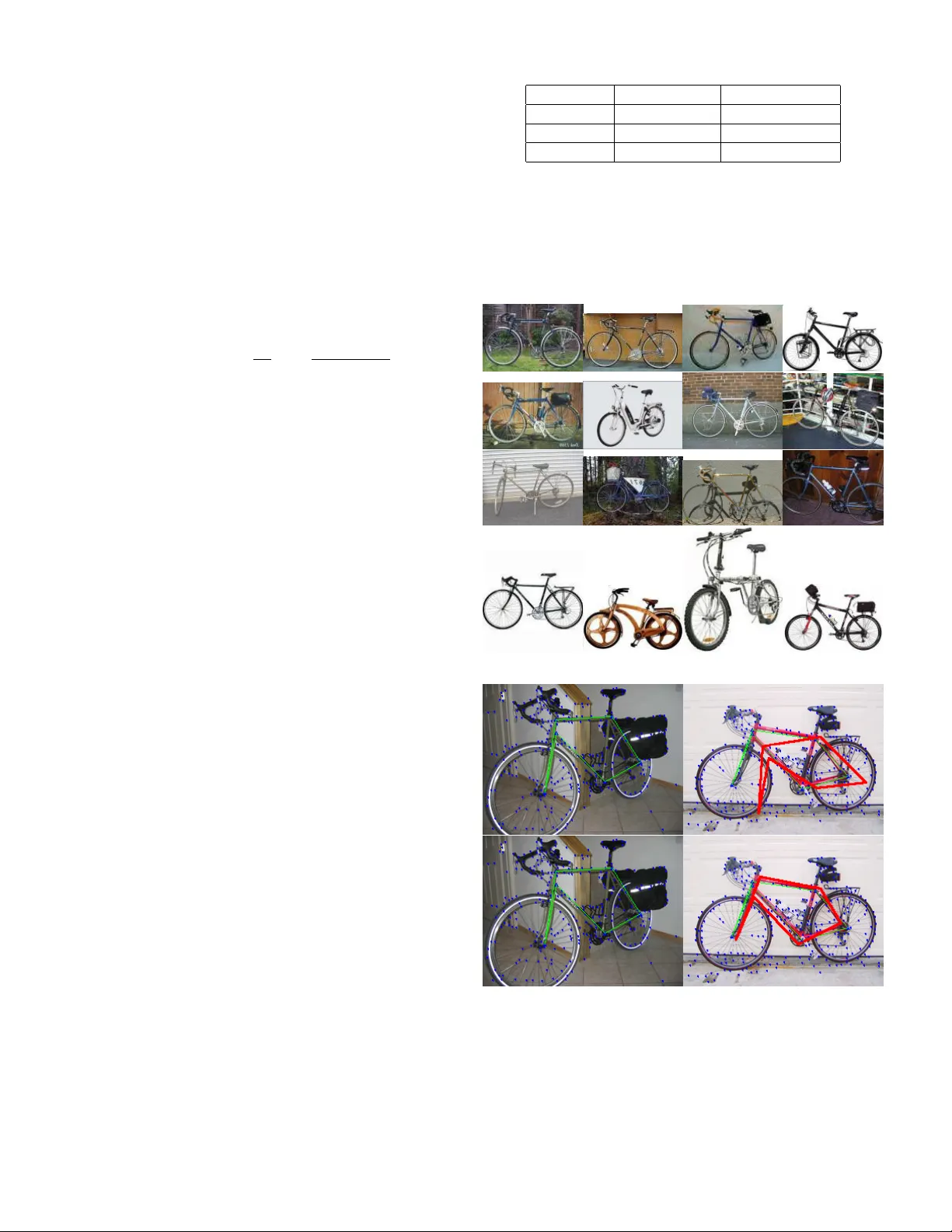
Learning Graph Matc hing Tib ´ erio S. Caetano, Julian J. McAuley , Li Cheng, Quo c V. Le and Alex J. Smola ∗ F ebruary 19, 2013 Abstract As a fundamen tal problem in pattern recognition, graph matc hing has applications in a v ariet y of fields, from com- puter vision to computational biology . In graph match- ing, patterns are modeled as graphs and pattern recognition amoun ts to finding a correspondence b etw een the nodes of differen t graphs. Many form ulations of this problem can b e cast in general as a quadratic assignment problem, where a linear term in the ob jectiv e function enco des no de compati- bilit y and a quadratic term encodes edge compatibility . The main researc h fo cus in this theme is about designing efficien t algorithms for approximately solving the quadratic assign- men t problem, since it is NP-hard. In this pap er we turn our atten tion to a different question: ho w to estimate compati- bilit y functions such that the solution of the resulting graph matc hing problem b est matc hes the exp ected solution that a human w ould manually pro vide. W e presen t a metho d for le arning gr aph matching : the training examples are pairs of graphs and the ‘labels’ are matc hes betw een them. Our exp erimen tal results reveal that learning can substan tially impro ve the performance of standard graph matching algo- rithms. In particular, we find that simple linear assignment with suc h a learning sc heme outp erforms Graduated As- signmen t with bisto chastic normalisation, a state-of-the-art quadratic assignmen t relaxation algorithm. 1 In tro duction Graphs are commonly used as abstract represen tations for complex structures, including DNA sequences, documents, text, and images. In particular they are extensively used in the field of computer vision, where man y problems can b e form ulated as an attributed graph matching problem. Here the no des of the graphs corresp ond to lo cal features of the image and edges corresp ond to relational asp ects b etw een features (b oth nodes and edges can b e attributed, i.e. they can encode feature v ectors). Graph matching then consists of finding a corresp ondence b etw een nodes of the t wo graphs suc h that they ’lo ok most similar’ when the vertices are lab eled according to suc h a correspondence. T ypically , the problem is mathematically formulated as a quadratic assignment problem, which consists of finding the assignmen t that maximizes an ob jective function en- ∗ Tib´ erio Caetano, Julian McAuley , Li Cheng, and Alex Smola are with the Statistical Mac hine Learning Program at NICT A, and the Research School of Information Sciences and Engineering, Australian National Universit y . Quoc Le is with the Department of Computer Science, Stanford Universit y . co ding lo cal compatibilities (a linear term) and structural compatibilities (a quadratic term). The main b o dy of re- searc h in graph matching has then b een foc used on devising more accurate and/or faster algorithms to solve the prob- lem approximately (since it is NP-hard); the compatibility functions used in graph matching are t ypically handcrafted. An interesting question arises in this context: If we are giv en t w o attributed graphs to matc h, G and G 0 , should the optimal matc h b e uniquely determined? F or example, assume first that G and G 0 come from t wo image s acquired b y a surveillance camera in an airp ort’s lounge; now, as- sume the same G and G 0 instead come from tw o images in a photographer’s image database; should the optimal matc h b e the same in both situations? If the algorithm takes into accoun t exclusiv ely the graphs to b e matched, the optimal solutions will b e the same 1 since the graph pair is the same in b oth cases. This is the standard w a y graph matc hing is approac hed to da y . In this pap er w e address what we believe to b e a limitation of this approach. W e argue that if we kno w the ‘conditions’ under whic h a pair of graphs has b een extracted, then w e should take in to account how gr aphs arising in those c on- ditions ar e typic al ly matche d . Ho wev er, w e do not tak e the information on the conditions explicitly into account, since this would obviously b e impractical. Instead, w e approac h the problem purely from a statistical inference p ersp ective. First, w e extract graphs from a n umber of images acquired under the same conditions as those for which w e w ant to solv e, whatev er the w ord ‘conditions’ means (e.g. from the surv eillance camera or the photographer’s database). W e then manual ly pro vide what we understand to b e the op- timal matc hes b et ween the resulting graphs. This informa- tion is then used in a le arning algorithm whic h learns a map from the space of pairs of graphs to the space of matc hes. In terms of the quadratic assignment problem, this learn- ing algorithm amounts to (in loose language) adjusting the no de and edge compatibility functions suc h that the ex- p ected optimal matc h in a test pair of graphs agrees with the exp ected match they w ould hav e had, had they b een in the training set. In this form ulation, the learning prob- lem consists of a con v ex, quadratic program whic h is readily solv able by means of a column generation pro cedure. W e pro vide exp erimental evidence that applying learn- ing to standard graph matc hing algorithms significantly im- pro ves their p erformance. In fact, w e show that learning impro ves up on non-learning results so dramatically that lin- ear assignment with le arning outp erforms Graduated As- 1 Assuming there is a single optimal solution and that the algorithm finds it. 1 signmen t with bisto chastic normalisation, a state-of-the-art quadratic assignment relaxation algorithm. Also, b y intro- ducing learning in Graduated Assignmen t itself, we obtain results that improv e b oth in accuracy and sp eed ov er the b est existing quadratic assignmen t relaxations. A preliminary version of this paper app eared in [1]. 1.1 Related Literature The graph matching literature is extensive, and many differ- en t types of approac hes hav e b een prop osed, which mainly fo cus on approximations and heuristics for the quadratic assignmen t problem. An incomplete list includes sp e c- tr al metho ds [2–6], r elaxation lab eling and pr ob abilistic appr o aches [7–13], semidefinite r elaxations [14], r eplic ator e quations [15], tr e e se ar ch [16], and gr aduate d assignment [17]. Sp ectral metho ds consist of studying the similarities b et ween the sp ectra of the adjacency or Laplacian matri- ces of the graphs and using them for matching. Relax- ation and probabilistic metho ds define a probabilit y dis- tribution ov er mappings, and optimize using discrete relax- ation algorithms or v ariants of b elief propagation. Semidef- inite relaxations solv e a con vex relaxation of the original com binatorial problem. Replicator equations draw an anal- ogy with mo dels from biology where an equilibrium state is sough t whic h solves a system of differen tial equations on the no des of the graphs. T ree-search techniques in general hav e w orst case exp onen tial complexit y and w ork via sequential tests of compatibilit y of local parts of the graphs. Gradu- ated Assignmen t combines the ‘softassign’ method [18] with Sinkhorn’s metho d [19] and essentially consists of a series of first-order approximations to the quadratic assignment ob jec tiv e function. This metho d is particularly p opular in computer vision since it produces accurate results while scaling reasonably in the size of the graph. The ab o ve literature strictly fo cuses on trying b etter algo- rithms for appro ximating a solution for the graph matching problem, but does not address the issue of ho w to determine the compatibilit y functions in a principled wa y . In [20] the authors learn compatibility functions for the relaxation lab eling pro cess; this is how ev er a different prob- lem than graph matc hing, and the ‘compatibility functions’ ha ve a different meaning. Nevertheless it do es provide an initial motiv ation for learning in the con text of matc hing tasks. In terms of methodology , the pap er most closely re- lated to ours is possibly [21], which uses structured estima- tion tools in a quadratic assignmen t setting for word align- men t. A recent paper of in terest shows that very significan t impro vemen ts on the performance of graph matc hing can be obtained b y an appropriate normalization of the compati- bilit y functions [22]; how ever, no learning is inv olved. 2 The Graph Matc hing Problem The notation used in this pap er is summarized in table 1. In the follo wing we denote a graph by G . W e will often refer to a p air of graphs, and the second graph in the pair will b e denoted b y G 0 . W e study the general case of attribute d graph matching, and attributes of the vertex i and the edge T able 1: Definitions and Notation G - generic graph (similarly , G 0 ); G i - attribute of no de i in G (similarly , G 0 i 0 for G 0 ); G ij - attribute of edge ij in G (similarly , G 0 i 0 j 0 for G 0 ); G - space of graphs ( G × G - space of pairs of graphs); x - generic observ ation: graph pair ( G, G 0 ); x ∈ X , space of observ ations; y - generic labe l: matching matrix; y ∈ Y , space of lab els; n - index for training instance; N - num b er of training in- stances; x n - n th training observ ation: graph pair ( G n , G 0 n ); y n - n th training label: matching matrix; g - predictor function; y w - optimal prediction for g under w ; f - discriminant function; ∆ - loss function; Φ - joint feature map; φ 1 - node feature map; φ 2 - edge feature map; S n - constrain t set for training instance n ; y ∗ - solution of the quadratic assignment problem; ˆ y - most violated constrain t in column generation; y ii 0 - i th ro w and i 0 th column elemen t of y ; c ii 0 - v alue of compatibility function for map i 7→ i 0 ; d ii 0 j j 0 - v alue of compatibility function for map ij 7→ i 0 j 0 ;  - tolerance for column generation; w 1 - no de parameter v ector; w 2 - edge parameter vector; w := [ w 1 w 2 ] - joint parameter vector; w ∈ W ; ξ n - slac k v ariable for training instance n ; Ω - regularization function; λ - regularization parameter; δ - conv ergence monitoring threshold in bisto chastic nor- malization. 2 ij in G are denoted by G i and G ij resp ectiv ely . Standard graphs are obtained if the no de attributes are empty and the edge attributes G ij ∈ { 0 , 1 } are binary denoting the absence or presence of an edge, in which case we get the so-called exact graph matching problem. Define a matching matrix y b y y ii 0 ∈ { 0 , 1 } such that y ii 0 = 1 if no de i in the first graph maps to node i 0 in the second graph ( i 7→ i 0 ) and y ii 0 = 0 otherwise. Define by c ii 0 the v alue of the compatibility function for the unary assignmen t i 7→ i 0 and b y d ii 0 j j 0 the v alue of the compati- bilit y function for the pairwise assignment ij 7→ i 0 j 0 . Then, a generic form ulation of the graph matching problem con- sists of finding the optimal matching matrix y ∗ giv en by the solution of the following (NP-hard) quadr atic assignment pr oblem [23] y ∗ = argmax y   X ii 0 c ii 0 y ii 0 + X ii 0 j j 0 d ii 0 j j 0 y ii 0 y j j 0   , (1) t ypically sub ject to either the injectivit y constrain t (one- to-one, that is P i y ii 0 ≤ 1 for all i 0 , P i 0 y ii 0 ≤ 1 for all i ) or simply the constraint that the map should b e a function (man y-to-one, that is P i 0 y ii 0 = 1 for all i ). If d ii 0 j j 0 = 0 for all ii 0 j j 0 then (1) b ecomes a line ar assignment pr oblem , exactly solv able in worst case cubic time [24]. Although the compatibilit y functions c and d obviously dep end on the at- tributes { G i , G 0 i 0 } and { G ij , G 0 i 0 j 0 } , the functional form of this dep endency is typically assumed to b e fixed in graph matc hing. This is precisely the restriction we are going to relax in this pap er: b oth the functions c and d will b e parametrized by vectors whose co efficients will b e learned within a conv ex optimization framew ork. In a w ay , instead of prop osing y et another algorithm for determining how to appro ximate the solution for (1), w e are aiming at finding a wa y to determine what should be maximized in (1), since differen t c and d will produce different criteria to be maxi- mized. 3 Learning Graph Matc hing 3.1 General Problem Setting W e approach the problem of learnin g the compatibility func- tions for graph matching as a sup ervised learning problem [25]. The training set comprises N observ ations x from an input set X , N corresp onding lab els y from an output set Y , and can be represented b y { ( x 1 ; y 1 ) , . . . , ( x N ; y N ) } . Critical in our setting is the fact that the observ ations and labels are structur e d obje cts . In t ypical sup ervised learning scenarios, observ ations are v ectors and lab els are elemen ts from some discrete set of small cardinality , for example y n ∈ {− 1 , 1 } in the case of binary classification. How ev er, in our case an observ ation x n is a p air of gr aphs , i.e. x n = ( G n , G 0 n ), and the lab el y n is a match b etw een graphs, represented b y a matc hing matrix as defined in section 2. If X = G × G is the space of pairs of graphs, Y is the space of matc hing matrices, and W is the space of parameters of our mo del, then learning graph matching amounts to estimating a function g : G × G × W 7→ Y which minimizes the prediction loss on the test set. Since the test set here is assumed not to b e av ailable at training time, w e use the standard approach of minimizing the empirical risk (a verage loss in the training set) plus a regularization term in order to a void ov erfitting. The optimal predictor will then b e the one which minimizes an expression of the follo wing t yp e: 1 N N X n =1 ∆( g ( G n , G 0 n ; w ) , y n ) | {z } empirical risk + λ Ω( w ) | {z } regularization term , (2) where ∆( g ( G n , G 0 n ; w ) , y n ) is the loss incurred b y the pre- dictor g when predicting, for training input ( G n , G 0 n ), the output g ( G n , G 0 n ; w ) instead of the training output y n . The function Ω( w ) p enalizes ‘complex’ vectors w , and λ is a pa- rameter that trades off data fitting against generalization abilit y , whic h is in practice determined using a v alidation set. In order to completely sp ecify suc h an optimization problem, we need to define the parametrized class of predic- tors g ( G, G 0 ; w ) whose paramete rs w w e will optimize ov er, the loss function ∆ and the regularization term Ω( w ). In the following w e will fo cus on setting up the optimization problem b y addressing each of these points. 3.2 The Mo del W e start b y specifying a w -parametrized class of predictors g ( G, G 0 ; w ). W e use the standard approach of discriminant functions, which consists of picking as our optimal estimate the one for which the discriminan t function f ( G, G 0 , y ; w ) is maximal, i.e. g ( G, G 0 ; w ) = argmax y f ( G, G 0 , y ; w ). W e assume linear discriminan t functions f ( G, G 0 , y ; w ) = h w , Φ( G, G 0 , y ) i , so that our predictor has the form g ( G, G 0 , w ) = argmax y ∈ Y h w , Φ( G, G 0 , y ) i . (3) Effectiv ely we are solving an in verse optimization problem, as described by [25, 26], that is, we are trying to find f suc h that g has desirable prop erties. F urther specification of g ( G, G 0 ; w ) requires determining the join t feature map Φ( G, G 0 , y ), whic h has to enco de the prop erties of b oth graphs as well as the prop erties of a match y b etw een these graphs. The key observ ation here is that we can relate the quadratic assignment form ulation of graph matching, given b y (1), with the predictor given by (3), and interpret the solution of the graph matching problem as b eing the esti- mate of g , i.e. y w = g ( G, G 0 ; w ). This allows us to interpret the discriminant function in (3) as the ob jective function to b e maximized in (1): h Φ( G, G 0 , y ) , w i = X ii 0 c ii 0 y ii 0 + X ii 0 j j 0 d ii 0 j j 0 y ii 0 y j j 0 . (4) This clearly reveals that the graphs and the parameters m ust b e enco ded in the compatibility functions. The last step b efore obtaining Φ consists of c ho osing a parametriza- tion for the compatibility functions. W e assume a simple 3 linear parametrization c ii 0 = h φ 1 ( G i , G 0 i 0 ) , w 1 i (5a) d ii 0 j j 0 =  φ 2 ( G ij , G 0 i 0 j 0 ) , w 2  , (5b) i.e. the compatibilit y functions are linearly dependent on the parameters, and on new feature maps φ 1 and φ 2 that only in volv e the graphs (section 4 sp ecifies the feature maps φ 1 and φ 2 ). As already defined, G i is the attribute of no de i and G ij is the attribute of edge ij (similarly for G 0 ). How- ev er, w e stress here that these are not necessarily lo c al at- tributes, but are arbitrary features simply indexe d by the no des and edges. 2 F or instance, w e will see in section 4 an example where G i enco des the graph structure of G as ‘seen’ from node i , or from the ‘persp ective’ of no de i . Note that the traditional wa y in which graph matc hing is approached arises as a particular case of equations (5): if w 1 and w 2 are constan ts, then c ii 0 and d ii 0 j j 0 dep end only on the features of the graphs. By defining w := [ w 1 w 2 ], we arriv e at the final form for Φ( G, G 0 , y ) from (4) and (5): Φ( G, G 0 , y ) = " X ii 0 y ii 0 φ 1 ( G i , G 0 i 0 ) , X ii 0 j j 0 y ii 0 y j j 0 φ 2 ( G ij , G 0 i 0 j 0 ) # . (6) Naturally , the final sp ecification of the predictor g depends on the choices of φ 1 and φ 2 . Since our exp erimen ts are con- cen trated on the computer vision domain, we use typical computer vision features (e.g. Shape Con text) for construct- ing φ 1 and a simple edge-match criterion for constructing φ 2 (details follo w in section 4). 3.3 The Loss Next we define the loss ∆( y , y n ) incurred by estimating the matc hing matrix y instead of the correct one, y n . When b oth graphs ha ve large sizes, w e define this as the fraction of mismatc hes betw een matrices y and y n , i.e. ∆( y , y n ) = 1 − 1 k y n k 2 F X ii 0 y ii 0 y n ii 0 . (7) (where k·k F is the F rob enius norm). If one of the graphs has a small size, this measure may b e to o rough. In our ex- p erimen ts w e will encoun ter suc h a situation in the con text of matching in images. In this case, we instead use the loss ∆( G, G 0 , π ) = 1 − 1 | π | X i " d ( G i , G 0 π ( i ) ) σ # . (8) Here graph no des corresp ond to p oint sets in the images, G corresp onds to the smaller, ‘query’ graph, and G 0 is the larger, ‘target’ graph (in this expression, G i and G 0 j are par- ticular p oints in G and G 0 ; π ( i ) is the index of the p oin t in 2 As a result in our general setting ‘no de’ compatibilities and ‘edge’ compatibilities b ecome somewhat misnomers, being more appropri- ately describ ed as unary and binary compatibilities. W e howev er stic k to the standard terminology for simplicity of exp osition. G 0 to which the i th p oin t in G should b e correctly mapped; d is simply the Euclidean distance, and is scaled b y σ , whic h is simply the width of the image in question). Hence we are p enalising matches based on how distant they are from the correct matc h; this is commonly referred to as the ‘endpoint error’. Finally , w e sp ecify a quadratic regularizer Ω( w ) = 1 2 k w k 2 . 3.4 The Optimization Problem Here w e com bine the elemen ts discussed in 3.2 in order to formally set up a mathematical optimization problem that corresp onds to the learning pro cedure. The expression that arises from (2) by incorp orating the sp ecifics discussed in 3.2 / 3.3 still consists of a very difficult (in particular non- con vex) optimization problem. Although the regulariza- tion term is conv ex in the parameters w , the empirical risk, i.e. the first term in (2), is not. Note that there is a finite n umber of p ossible matc hes y , and therefore a finite n um- b er of p ossible v alues for the loss ∆; how ever, the space of parameters W is contin uous. What this means is that there are large equiv alence classes of w (an equiv alence class in this case is a given set of w ’s each of which pro duces the same loss). Therefore, the loss is piecewise constan t on w , and as a result certainly not amenable to an y t yp e of smo oth optimization. One approach to render the problem of minimizing (2) more tractable is to replace the empirical risk by a con vex upp er b ound on the empirical risk, an idea that has b een exploited in Mac hine Learning in recent years [25, 27, 28]. By minimizing this con vex upper b ound, we hope to decrease the empirical risk as w ell. It is easy to show that the con vex (in particular, linear) function 1 N P n ξ n is an upper b ound for 1 N P n ∆( g ( G n , G 0 n ; w ) , y n ) for the solution of (2) with appropriately c hosen constrain ts: minimize w,ξ 1 N N X n =1 ξ n + λ 2 k w k 2 (9a) sub jec t to h w , Ψ n ( y ) i ≥ ∆( y , y n ) − ξ n (9b) for all n and y ∈ Y . Here w e define Ψ n ( y ) := Φ( G n , G 0 n , y n ) − Φ( G n , G 0 n , y ). F ormally , w e ha ve: Lemma 3.1 F or any fe asible ( ξ , w ) of (9) the ine quality ξ n ≥ ∆( g ( G n , G 0 n ; w ) , y n ) holds for al l n . In p articu- lar, for the optimal solution ( ξ ∗ , w ∗ ) we have 1 N P n ξ ∗ n ≥ 1 N P n ∆( g ( G n , G 0 n ; w ∗ ) , y n ) . Pro of The constraint (9b) needs to hold for all y , hence in particular for y w ∗ = g ( G n , G 0 n ; w ∗ ). By construction y w ∗ satisfies  w , Ψ n ( y w ∗ )  ≤ 0. Consequently ξ n ≥ ∆( y w ∗ , y n ). The second part of the claim follows immediately . The constrain ts (9b) mean that the margin f ( G n , G 0 n , y n ; w ) − f ( G n , G 0 n , y ; w ), i.e. the gap b e- t ween the discriminant functions for y n and y should exceed the loss induced by estimating y instead of the 4 training matching matrix y n . This is highly in tuitive since it reflects the fact that we wan t to safeguard ourselves most against mis-predictions y which incur a large loss (i.e. the smaller is the loss, the less we should care ab out making a mis-prediction, so we can enforce a smaller margin). The presence of ξ n in the constrain ts and in the ob jectiv e function means that we allo w the hard inequality (without ξ n ) to b e violated, but we penalize violations for a giv en n b y adding to the ob jectiv e function the cost 1 N ξ n . Despite the fact that (9) has exp onentially many con- strain ts (ev ery p ossible matc hing y is a constraint), we will see in what follo ws that there is an efficient wa y of finding an  -appro ximation to the optimal solution of (9) by finding the worst violators of the constrained optimization problem. 3.5 The Algorithm Note that the n umber of constraints in (9) is given by the n umber of p ossible matc hing matrices | Y | times the num b er of training instances N . In graph matching the num b er of p ossible matches b et ween tw o graphs gro ws factorially with their size. In this case it is infeasible to solve (9) exactly . There is ho wev er a wa y out of this problem b y using an optimization tec hnique kno wn as c olumn gener ation [24]. Instead of solving (9) directly , one computes the most vi- olated constrain t in (9) iterativ ely for the current solution and adds this constraint to the optimization problem. In order to do so, w e need to solve argmax y [ h w , Φ( G n , G 0 n , y ) i + ∆( y , y n )] , (10) as this is the term for whic h the constrain t (9b) is tightest (i.e. the constraint that maximizes ξ n ). The resulting algorithm is given in algorithm 1. W e use the ’Bundle Methods for Regularized Risk Minimization’ (BMRM) solver of [29], which merely requires that for each candidate w , w e compute the gradien t of 1 N P h w , Ψ( ˆ y ) i + λ 2 k w k 2 with resp ect to w , and the loss ( 1 N P n ∆( ˆ y , y n )) ( ˆ y is the most violated constrain t in column generation). See [29] for further details Let us inv estigate the complexit y of solving (10). Using the joint feature map Φ as in (6) and the loss as in (7), the argumen t in (10) b ecomes h Φ( G, G 0 , y ) , w i + ∆( y , y n ) = (11) = X ii 0 y ii 0 ¯ c ii 0 + X ii 0 j j 0 y ii 0 y j j 0 d ii 0 j j 0 + constant , where ¯ c ii 0 = h φ 1 ( G i , G 0 i 0 ) , w 1 i + y n ii 0 / k y n k 2 F and d ii 0 j j 0 is defined as in (5b). The maximization of (11), which needs to be carried out at tr aining time, is a quadratic assignment problem, as is the problem to be solved at test time. In the particular case where d ii 0 j j 0 = 0 throughout, b oth the problems at training and at test time are linear assignment problems, whic h can b e solv ed efficien tly in worst case cubic time. In our exp eriments, we solve the linear assignmen t prob- lem with the efficient solver from [30] (‘house’ sequence), and the Hungarian algorithm (video/bikes dataset). F or Algorithm 1 Column Generation Define: Ψ n ( y ) := Φ( G n , G 0 n , y n ) − Φ( G n , G 0 n , y ) H n ( y ) := h w , Φ( G n , G 0 n , y ) i + ∆( y , y n ) Input: training graph pairs { G n } , { G 0 n } , training match- ing matrices { y n } , sample size N , tolerance  Initialize S n = ∅ for all n , and w = 0 rep eat Get curren t w from BMRM for n = 1 to N do ˆ y = argmax y ∈ Y H n ( y ) Compute gradien t of h w , Ψ( G n , G 0 n , y ) i + λ 2 k w k 2 w.r.t. w (= Ψ n ( ˆ y ) + λw ) Compute loss ∆( ˆ y , y n ) end for Rep ort 1 N P ξ n and 1 N P n ∆( ˆ y , y n ) to BMRM un til 1 N P ξ n is sufficien tly small quadratic assignmen t, we dev elop ed a C++ implemen tation of the w ell-known Graduated Assignmen t algorithm [17]. Ho wev er the learning scheme discussed here is indep en- den t of whic h algorithm w e use for solving either linear or quadratic assignmen t. Note that the estimator is bu t a mere appro ximation in the case of quadratic assignment: since w e are unable to find the most violated constraints of (10), we cannot be sure that the dualit y gap is prop erly minimized in the constrained optimization problem. 4 F eatures for the Compatibilit y F unctions The join t feature map Φ( G, G 0 , y ) has b een deriv ed in its full generalit y (6), but in order to hav e a working mo del w e need to c ho ose a sp ecific form for φ 1 ( G i , G 0 i 0 ) and φ 2 ( G ij , G 0 i 0 j 0 ), as mentioned in section 3. W e first discuss the linear fea- tures φ 1 and then pro ceed to the quadratic terms φ 2 . F or concreteness, here w e only discuss options actually used in our experiments. 4.1 No de F eatures W e construct φ 1 ( G i , G 0 i 0 ) using the squared difference φ 1 ( G i , G 0 i 0 ) = ( . . . , −| G i ( r ) − G 0 i 0 ( r ) | 2 , . . . ). This differs from what is shown in [1], in which an exp onential de- ca y is used (i.e. exp( −| G i ( r ) − G 0 i 0 ( r ) | 2 / )); we found that using the squared difference resulted in muc h b etter p er- formance after learning. Here G i ( r ) and G 0 i 0 ( r ) denote the r th co ordinates of the corresponding attribute v ectors. Note that in standard graph matc hing without learning w e typically ha v e c ii 0 = exp( − k G i − G 0 i 0 k 2 ), which can b e seen as the particular case of (5a) for b oth φ 1 and w 1 flat, given by φ 1 ( G i , G 0 i 0 ) = ( . . . , exp( − k G i − G 0 i 0 k 2 ) , . . . ) and w 1 = ( . . . , 1 , . . . ) [22]. Here instead w e ha ve c ii 0 = h φ 1 ( G i , G 0 i 0 ) , w 1 i , where w 1 is learned from training data. In this wa y , by tuning the r th co ordinate of w 1 accordingly , the learning pro cess finds the relev ance of the r th feature 5 of φ 1 . In our exp eriments (to be describ ed in the next sec- tion), we use the w ell-known 60-dimensional Shap e Con- text features [31]. They enco de how each no de ‘sees’ the other nodes. It is an instance of what w e called in sec- tion 3 a feature that captures the no de ‘p ersp ectiv e’ with resp ect to the graph. W e use 12 angular bins (for an- gles in [0 , π 6 ) . . . [ 11 π 6 , 2 π )), and 5 radial bins (for radii in (0 , 0 . 125) , [0 . 125 , 0 . 25) . . . [1 , 2), where the radius is scaled b y the av erage of all distances in the scene) to obtain our 60 features. This is similar to the setting describ ed in [31]. 4.2 Edge F eatures F or the edge features G ij ( G 0 i 0 j 0 ), we use standard graphs, i.e. G ij ( G 0 i 0 j 0 ) is 1 if there is an edge b et ween i and j and 0 otherwise. In this case, we set φ 2 ( G ij , G 0 i 0 j 0 ) = G ij G 0 i 0 j 0 (so that w 2 is a scalar). 5 Exp erimen ts 5.1 House Sequence F or our first exp eriment, we consider the CMU ‘house’ se- quence – a dataset consisting of 111 frames of a toy house [32]. Each frame in this sequence has b een hand-lab elled, with the same 30 landmarks identified in each frame [33]. W e explore the p erformance of our method as the baseline (separation betw een frames) v aries. F or eac h baseline (from 0 to 90, b y 10), w e iden tified all pairs of images separated by exactly this many frames. W e then split these pairs in to three sets, for training, v alidation, and testing. In order to determine the adjacency matrix for our edge features, w e triangulated the set of landmarks using the Delaunay triangulation (see figure 1). Figure 1 (top) sho ws the p erformance of our method as the baseline increases, for b oth linear and quadratic assign- men t (for quadratic assignment we use the Graduated As- signmen t algorithm, as men tioned previously). The v alues sho wn rep ort the normalised Hamming loss (i.e. the prop or- tion of points incorrectly matched); the regularization con- stan t resulting in the best p erformance on our v alidation set is used for testing. Graduated assignment using bisto chas- tic normalisation, which to the b est of our kno wledge is the state-of-the-art relaxation, is shown for comparison [22]. 3 F or b oth linear and quadratic assignment, figure 1 sho ws that learning significan tly outp erforms non-learning in terms of accuracy . In terestingly , quadratic assignment p erforms worse than linear assignment b efore learning is applied – this is likely b ecause the relativ e scale of the linear and quadratic features is badly tuned before learning. In- deed, this demonstrates exactly wh y learning is important. It is also worth noting that linear assignmen t with learning p erforms similarly to quadratic assignmen t with bisto chas- tic normalisation (without learning) – this is an important result, since quadratic assignmen t via Graduated Assign- men t is significan tly more computationally intensiv e. 3 Exponential decay on the no de features was beneficial when using the method of [22], and has hence been maintained in this case (see section 4.1); a normalisation constant of δ = 0 . 00001 was used. Figure 1: T op: Performance on the ‘house’ sequence as the baseline (separation b etw een frames) v aries (the nor- malised Hamming loss on all testing examples is reported, with error bars indicating the standard error). Centre: The w eights learned for the quadratic mo del (baseline = 90, λ = 1). Bottom: A frame from the sequence, together with its landmarks and triangulation; the 3 rd and the 93 rd frames, matched using linear assignmen t (without learning, loss = 12 / 30), and the same matc h after learning ( λ = 10, loss = 6 / 30). Mismatches are sho wn in red. 6 Figure 2: T op: Performance on the video se quence as the baseline (separation b et ween frames) v aries (the endp oin t error on all testing examples is rep orted, with error bars indicating the standard error). Centre: The w eights learned for the mo del (baseline = 90, λ = 100). Bottom: The 7 th and the 97 th frames, matc hed using linear assignmen t (loss = 0 . 028), and the same matc h after learning ( λ = 100, loss = 0 . 009). The outline of the points to b e matched (left), and the correct match (righ t) are shown in green; the inferred matc h is outlined in red; the matc h after learning is m uch closer to the correct matc h. Figure 3: Running time versus accuracy on the ‘house’ dataset, for a baseline of 90. Standard errors of b oth run- ning time and p erformance are shown (the standard error for the running time is almost zero). Note that linear as- signmen t is around three orders of magnitude faster than quadratic assignmen t. Figure 1 (centre) shows the weigh t vector learned us- ing quadratic assignmen t (for a baseline of 90 frames, with λ = 1). Note that the first 60 points sho w the w eights of the Shap e Con text features, whereas the final p oin t corresponds to the edge features. The final p oin t is given a very high score after learning, indicating that the edge features are imp ortan t in this mo del. 4 Here the first 12 features corre- sp ond to the first radial bin (as described in section 4) etc. The first radial bin appears to b e more imp ortant than the last, for example. Figure 1 (b ottom) also shows an example matc h, using the 3 rd and the 93 rd frames of the sequence for linear assignment, b efore and after learning. Finally , Figure 3 sho ws the running time of our metho d compared to its accuracy . Firstly , it should be noted that the use of learning has no effect on running time; since learn- ing outp erforms non-learning in all cases, this presents a v ery strong case for learning. Quadratic assignment with bisto c hastic normalisation gives the best non-learning per- formance, how ever, it is still worse than either linear or quadratic assignment with learning and it is significantly slo wer. 5.2 Video Sequence F or our second exp erimen t, we consider matc hing features of a h uman in a video sequence. W e used a video sequence from the SAMPL dataset [34] – a 108 frame sequence of a h uman face (see figure 2, b ottom). T o iden tify landmarks for these scenes, we used the SUSAN corner detector [35, 36]. This detector essentially identifies p oints as corners if their neighbours within a small radius are dissimilar. This 4 This should be in terpreted with some caution: the features hav e different scales, meaning that their imp ortances cannot be compared directly . Ho wev er, from the p oint of view of the regularizer, assigning this feature a high w eight bares a high cost, implying that it is an important feature. 7 detector was tuned suc h that no more than 200 landmarks w ere identified in eac h scene. In this setting, we are no longer in terested in matc hing al l of the landmarks in b oth images, but rather those that cor- resp ond to imp ortant parts of the human figure. W e iden ti- fied the same 11 p oints in each image (figure 2, b ottom). It is assumed that these points are kno wn in adv ance for the template scene ( G ), and are to b e found in the target scene ( G 0 ). Clearly , since the correct match corresp onds to only a tin y proportion of the scene, using the normalised Hamming loss is no longer appropriate – w e wish to p enalise incorrect matc hes less if they are ‘close to’ the correct match. Hence w e use the loss function (as introduced in section 3.2) ∆( G, G 0 , π ) = 1 − 1 | π | X i " d ( G i , G 0 π ( i ) ) σ # . (12) Here the loss is small if the distance b etw een the chosen matc h and the correct match is small. Since we are interested in only a few of our landmarks, triangulating the graph is no longer meaningful. Hence we presen t results only for linear assignmen t. Figure 2 (top) sho ws the p erformance of our method as the base line increases. In this case, the p erformance is non- monotonic as the sub ject mov es in and out of view through- out the sequence. This sequence presents additional difficul- ties o ver the ‘house’ dataset, as we are sub ject to noise in the detected landmarks, and p ossibly in their lab elling also. Nev ertheless, learning outp erforms non-learning for all base- lines. The w eigh t v ector (figure 2, cen tre) is heavily p eak ed ab out particular angular bins. 5.3 Bik es F or our final exp eriment, w e used images from the Caltech 256 dataset [37]. W e chose to matc h images in the ‘touring bik e’ class, which con tains 110 images of bicycles. Since the Shap e Context features we are using are robust to only a small amount of rotation (and not to reflection), we only included images in this dataset that were taken ‘side-on’. Some of these were then reflected to ensure that each im- age had a consistent orien tation (in total, 78 images re- mained). Again, the SUSAN corner detector was used to iden tify the landmarks in eac h scene; 6 p oints corresp ond- ing to the frame of the bicycle were identified in each frame (see figure 4, b ottom). Rather than matc hing all p airs of bicycles, w e used a fixed template ( G ), and only v aried the target. This is an easier problem than matching all pairs, but is realistic in many scenarios, suc h as image retriev al. T able 2 shows the endpoint error of our metho d, and gives further evidence of the improv ement of learning ov er non- learning. Figure 4 shows a selection of data from our train- ing set, as w ell as an example matching, with and without learning. Loss Loss (learning) T raining 0.094 (0.005) 0.057 (0.004) V alidation 0.040 (0.007) 0.040 (0.006) T esting 0.101 (0.005) 0.062 (0.004) T able 2: Performance on the ‘bikes’ dataset. Results for the minimiser of the v alidation loss ( λ = 10000) are reported. Standard errors are in paren theses. Figure 4: T op: Some of our training scenes. Bottom: A matc h from our test set. The top frame shows the p oin ts as matc hed without learning (loss = 0 . 105), and the b ottom frame shows the match with learning (loss = 0 . 038). The outline of the p oints to be matc hed (left), and the correct matc h (right) are outlined in green; the inferred match is outlined in red. 8 6 Conclusions and Discussion W e hav e shown how the compatibility functions for the graph matching problem can b e estimated from lab eled training examples, where a training input is a pair of graphs and a training output is a matc hing matrix. W e use large- margin structured estimation techniques with column gen- eration in order to solv e the learning problem efficien tly , despite the h uge num b er of constraints in the optimization problem. W e presented exp erimental results in three differ- en t settings, eac h of which revealed that the graph matching problem can b e significan tly impro ved b y means of learning. An interesting finding in this w ork has b een that line ar assignmen t with learning p erforms similarly to Graduated Assignmen t with bisto chastic normalisation, a state-of-the- art quadr atic assignment relaxation algorithm. This sug- gests that, in situations where sp eed is a ma jor issue, lin- ear assignment may b e resurrected as a means for graph matc hing. In addition to that, if learning is introduced to Graduated Assignment itself , then the p erformance of graph matc hing impr oves signific antly both on accuracy and sp eed when compared to the b est existing quadratic assignment relaxation [22]. There are many other situations in which learning a matc hing criterion can be useful. In multi-camera settings for example, when different cameras may be of different t yp es and hav e different calibrations and viewp oin ts, it is reasonable to exp ect that the optimal compatibilit y func- tions will be different dep ending on which camera pair we consider. In surv eillance applications w e should tak e adv an- tage of the fact that muc h of the con text does not c hange: the camera and the viewpoint are typically the same. T o summarize, b y learning a matching criterion from pre- viously lab eled data, we are able to substantially impro ve the accuracy of graph matc hing algorithms. References [1] T. S. Caetano, L. Cheng, Q. V. Le, and A. J. Smola, “Learning graph matching,” in International Confer- enc e on Computer Vision , 2007. [2] M. Leordean u and M. Heb ert, “A sp ectral technique for corresp ondence problems using pairwise constraints,” in ICCV , 2005. [3] H. W ang and E. R. Hanco ck, “A k ernel view of spectral p oin t pattern matc hing,” in International Workshops SSPR & SPR, LNCS 3138 , 2004, pp. 361–369. [4] L. Shapiro and J. Brady , “F eature-based corresp on- dence - an eigen vector approach,” Image and Vision Computing , v ol. 10, pp. 283–288, 1992. [5] M. Carcassoni and E. R. Hanco c k, “Spectral correspon- dence for p oin t pattern matching,” Pattern R e c o gni- tion , v ol. 36, pp. 193–204, 2003. [6] T. Caelli and S. Kosino v, “An eigenspace pro jection clustering metho d for inexact graph matching,” IEEE T r ans. P AMI , v ol. 26, no. 4, pp. 515–519, 2004. [7] T. S. Caetano, T. Caelli, and D. A. C. Barone, “Graph- ical mo dels for graph matc hing,” in IEEE International Confer enc e on Computer Vision and Pattern R e c o gni- tion , W ashington, DC, 2004, pp. 466–473. [8] A. Rosenfeld and A. C. Kak, Digital Pictur e Pr o c essing . New Y ork, NY: Academic Press, 1982. [9] R. C. Wilson and E. R. Hancock, “Structural matching b y discrete relaxation,” IEEE T r ans. P AMI , v ol. 19, no. 6, pp. 634–648, 1997. [10] E. Hanco c k and R. C. Wilson, “Graph-based metho ds for vision: A yorkist manifesto,” SSPR & SPR 2002, LNCS , v ol. 2396, pp. 31–46, 2002. [11] W. J. Christmas, J. Kittler, and M. P etrou, “Structural matc hing in computer vision using probabilistic relax- ation,” IEEE T r ans. P AMI , v ol. 17, no. 8, pp. 749–764, 1994. [12] J. V. Kittler and E. R. Hancock, “Combining evidence in probabilistic relaxation,” Int. Journal of Pattern R e c o gnition and Artificial Intel ligenc e , v ol. 3, pp. 29– 51, 1989. [13] S. Z. Li, “A marko v random field mo del for ob ject matc hing under contextual constraints,” in Interna- tional Confer enc e on Computer Vision and Pattern R e c o gnition , 1994, pp. 866–869. [14] C. Schellew ald, “Con vex mathematical programs for re- lational matching of ob ject views,” Ph.D. dissertation, Univ ersity of Mannhein, 2004. [15] M. P elillo, “Replicator equations, maximal cliques, and graph isomorphism,” Neur al Comput. , vol. 11, pp. 1933–1955, 1999. [16] B. T. Me ssmer and H. Bunke, “A new algorithm for error-toleran t subgraph isomorphism detection,” IEEE T r ans. P AMI , v ol. 20, no. 5, pp. 493–503, 1998. [17] S. Gold and A. Rangara jan, “A graduated assignmen t algorithm for graph matc hing,” IEEE T r ans. P AMI , v ol. 18, no. 4, pp. 377–388, 1996. [18] A. Rangara jan, A. Y uille, and E. Mjolsness, “Conv er- gence properties of the softassign quadratic assignmen t algorithm,” Neur al Computation , vol. 11, pp. 1455– 1474, 1999. [19] R. Sinkhorn, “A relationship b et ween arbitrary p ositive matrices and doubly sto chastic matrices,” Ann. Math. Statis. , v ol. 35, pp. 876–879, 1964. [20] M. Pelillo and M. Refice, “Learning compatibilit y co ef- ficien ts for relaxation lab eling pro cesses,” IEEE T r ans. on P AMI , v ol. 16, no. 9, pp. 933–945, 1994. [21] S. Lacoste-Julien, B. T ask ar, D. Klein, and M. Jordan, “W ord alignment via quadratic assignment,” in HL T- NAACL06 , 2006. 9 [22] T. Cour, P . Sriniv asan, and J. Shi, “Balanced graph matc hing,” in NIPS , 2006. [23] K. Anstreicher, “Recent adv ances in the solution of quadratic assignment problems,” Math. Pr o gr am., Ser. B , v ol. 97, pp. 27–42, 2003. [24] C. Papadimitriou and K. Steiglitz, Combinatorial Op- timization : A lgorithms and Complexity . Dov er Pub- lications, July 1998. [25] I. Tso chan taridis, T. Joachims, T. Hofmann, and Y. Al- tun, “Large margin metho ds for structured and interde- p enden t output v ariables,” J. Mach. L e arn. R es. , vol. 6, pp. 1453–1484, 2005. [26] R. K. Ahuja and J. B. Orlin, “Inv erse optimization,” Op er ations R ese ar ch , v ol. 49, no. 5, pp. 771–783, 2001. [27] A. Smola, S. V. N. Vish wanathan, and Q. Le, “Bundle metho ds for machine learning,” in A dvanc es in Neur al Information Pr o c essing Systems 20 , J. Platt, D. Koller, Y. Singer, and S. Ro weis, Eds. Cam bridge, MA: MIT Press, 2008, pp. 1377–1384. [28] B. T ask ar, C. Guestrin, and D. Koller, “Max-margin mark ov netw orks,” in A dvanc es in Neur al Informa- tion Pr o c essing Systems 16 , S. Thrun, L. Saul, and B. Sch¨ olk opf, Eds. Cambridge, MA: MIT Press, 2004. [29] C. T eo, Q. Le, A. Smola, and S. Vishw anathan, “A scalable mo dular con vex solver for regularized risk min- imization,” in Know le dge Disc overy and Data Mining KDD’07 , 2007. [30] R. Jonker and A. V olgenant, “A shortest augmen ting path algorithm for dense and sparse linear assignment problems,” Computing , v ol. 38, no. 4, pp. 325–340, 1987. [31] S. Belongie, J. Malik, and J. Puzicha, “Shape match- ing and ob ject recognition using shape contexts,” IEEE T r ans. on P AMI , vol. 24, no. 24, pp. 509–521, 2002. [32] CMU ‘house’ dataset: v asc.ri.cmu.edu/idb/h tml/motion/house/index.html. [33] T. S. Caetano, T. Caelli, D. Sch uurmans, and D. A. C. Barone, “Graphical mo dels and p oint pattern match- ing,” IEEE T r ans. on P AMI , vol. 28, no. 10, pp. 1646– 1663, 2006. [34] SAMPLE motion dataset: h ttp://sampl.ece.ohio-state.edu/database.htm. [35] S. Smith, “A new class of corner finder,” in BMVC , 1992, pp. 139–148. [36] ——, “Flexible filter neighbourho o d designation,” in ICPR , 1996, pp. 206–212. [37] G. Griffin, A. Holub, and P . Perona, “Caltech- 256 ob ject category dataset,” California Institute of T echnology , T ech. Rep. 7694, 2007. [Online]. Av ailable: h ttp://authors.library .caltech.edu/7694 10