How Many Users should be Turned On in a Multi-Antenna Broadcast Channel?

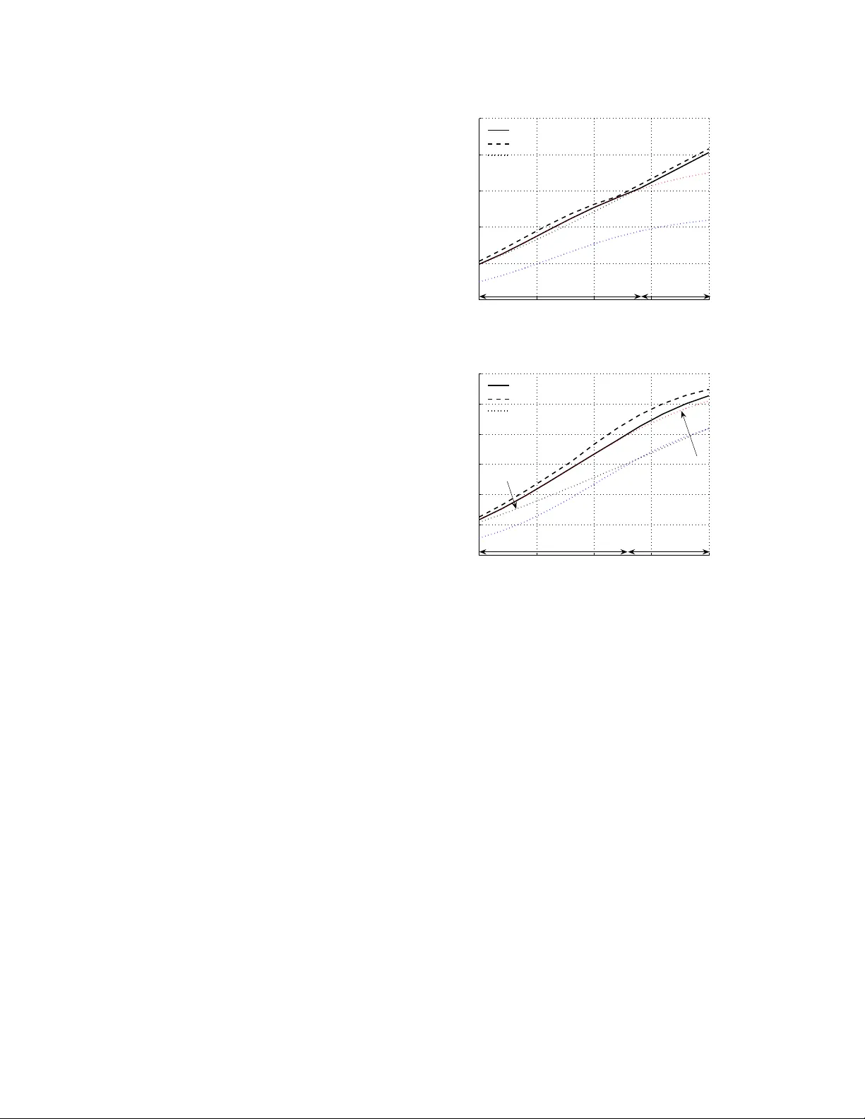
1 Ho w Man y Users should be T urned On in a Multi-Antenna Broadcast Channel? W ei Dai, Member , IEEE , Y oujian (Eugene) Liu, Member , IEEE , Brian C. Rider and W en Gao Abstract — This paper considers broadcast channels with L antennas at the base station and m single-antenna users, where L and m are typically of the same order . W e assume that only partial channel state information is a vailable at the base station through a finite rate feedback. Our key observation is that the optimal number of on-users (users turned on), say s , is a function of signal-to-noise ratio (SNR) and feedback rate. In support of this, an asymp- totic analysis is employed where L , m and the feedback rate approach infinity linearly . W e derive the asymptotic optimal feedback strategy as well as a realistic criterion to decide which users should be turned on. The corr esponding asymptotic thr oughput per antenna, which we define as the spatial efficiency , turns out to be a function of the number of on-users s , and theref ore s must be chosen appropriately . Based on the asymptotics, a scheme is de veloped f or systems with finite many antennas and users. Compared with other studies in which s is presumed constant, our scheme achieves a significant gain. Furthermore, our analysis and scheme are valid for heterogeneous systems wher e different users may have differ ent path loss coefficients and feedback rates. Index T erms — Broadcast channels, feedback, MIMO systems, throughput. I . I N T RO D U C T I O N It is well known that multiple antennas can improv e the spectral efficiency . This paper considers broadcast channels with L antennas at the base station and m single-antenna users. T o achiev e the full benefit, perfect channel state information (CSI) is required at both re- ceiv er and transmitter . Perfect CSI at the receiv er can be obtained by estimation from the receiv ed signal. How- ev er, if CSI at the transmitter (CSIT) is obtained from feedback, perfect CSIT requires an infinite feedback rate. As this is not feasible in practice, it is important to Manuscript recei ved No vember 1, 2007; revised April 15, 2008. This work was supported by NSF Grants DMS-0505680, CCF-0728955, ECCS-0725915, and Thomson Inc. Part of content was presented at the Conference on Information Sciences and Systems, Baltimore, MD, March 2007. W . Dai is with the Department of Electrical and Computer Engineer- ing, University of Illinois at Urbana-Champaign, Urbana, IL 61801, USA (email: wei.dai@colorado.edu). Y . Liu and B. C. Rider are with the Department of Electrical and Computer Engineering and the Department of Mathematics, respec- tiv ely , University of Colorado at Boulder , Boulder , CO 80309, USA (email: eugeneliu@ieee.org, brian.rider@colorado.edu). W . Gao is with Thomson Inc., T wo Independence W ay , Princeton, NJ 08540, USA (email:wen.gao@thomson.net). analyze the effect of finite rate feedback and design efficient strategy accordingly . The feedback models for broadcast channels are de- scribed as follows. T o sa ve feedback rate on po wer control, we assume a power on/off strategy 1 where each user is either turned on with a constant power or turned off. For a given channel realization, the users quantize their channel states into finite bits and feedback the corresponding indices to the base station. After receiving the feedback from users, the base station decides which users should be turned on and then forms beamforming vectors for transmission. Broadcast channels with feedback hav e been widely studied recently . Ideally , if the base station has the per- fect CSI, dirty paper codes or zero-forcing transmission can help clean off interference among users. Howe ver , with only finite rate feedback on CSI, the base station does not know the perfect channel state information and therefore interference from other users is inevitable. The interference gets so strong at high signal-to-noise ratio (SNR) regions that the system throughput is upper bounded by a constant even when SNR approaches infin- ity . This phenomena, called interference domination, was reported on in [1], [2]. One way to combat it is to allow the number of users to be much larger than the number of antennas at the base station. With sufficiently many independent realizations of the channel, it is possible to obtain L orthogonal users with feedback: Sharif and Hassibi select users whose channel directions are close to a random generated basis vectors in [1]; Y oo, et. al., pick up near orthogonal users in an iterativ e way [3], [4]. Recently , Bayesteh and Khandani quantified the feedback required as a function of the number of users [5], [6]. Another approach is to fix both the number of antennas at the base station and the system size (the number of users). It has been shown in [7] that the maximum achiev able multiplexing gain is one (at high SNR) with finite rate feedback. The full multiplexing gain requires the feedback rate increases linearly with SNR [2]. In both approaches, a homogeneous system is assumed where all the users share the same path loss coefficient and feedback resource. Separate from the above, this paper studies a more 1 This assumption will be further validated in Section II. 2 realistic scenario: • W e consider heterogeneous systems where different users may have different path loss coef ficients and feedback rates. • The size of the broadcast system is small. That is, the number of users and the number of antennas at the base station are typically of the same order . Note that a cooperati ve communication netw ork can often be viewed as a composition of multi-access and broadcast sub-systems with a small number of users. Research on broadcast systems of small size also provides insights into cooperativ e communica- tions. • Analysis and design are valid for arbitrary SNR. According to the authors’ knowledge, the above prac- tically important scenario has not been systematically studied due to the associated difficulty in analysis. For such systems, we solve the interference domina- tion problem by choosing the appropriate number of on- users s . This solution comes from an asymptotic analysis where L, m, s and the feedback rates approach infinity linearly . As hav e been demonstrated in [8] and will be verified in our simulations in Fig. 1, this type of asymptotic analysis is surprisingly reliable when being applied to small systems. The main asymptotic results include: • It is asymptotically optimal to only quantize the channel directions and ignore the channel magni- tude information. The asymptotically optimal feed- back function and codebook are deriv ed accord- ingly . • A realistic on/off criterion is proposed to decide which users should be turned on. • The corresponding throughput per antenna con- ver ges to a constant, defined as the spatial effi- ciency . It is a function of the normalized number of on-users ¯ s = s L . Further , there exists a unique ¯ s ∈ (0 , 1) to maximize the the spatial efficienc y . Based on the insights obtained from the above asymp- totic results, we develop a scheme to choose the appro- priate s for systems with finite L and m . Simulations show that the gain achiev ed by choosing s is significant compared with the strate gies where s = L [2]. In addition, our scheme has the following advantages. • It is valid for heterogeneous systems. • The associated computation complexity is low . In the proposed scheme, the choice of on-users is in- dependent of the channel realization, and therefore there is no need to select on-users e very fading block. The computation complexity is much smaller than that of user selection [1], [5], [6]. • Only on-users need to feedback CSI, which saves the precious feedback resource. I I . S Y S T E M M O D E L Consider a broadcast channel with L antennas at the base station and m single-antenna users. Assume that the base station employs zero forcing transmitter . Let γ i ≥ 0 ( 1 ≤ i ≤ m ) be the path loss coefficient for user i . Then the recei ved signal Y i ∈ C for user i is giv en by Y i = √ γ i h † i   m X j =1 q j X j   + W i , where h i ∈ C L × 1 is the channel state vector for user , q j ∈ C L × 1 is the zero-forcing beamforming vector for user j , X j ∈ C is the source signal for the user j and W i ∈ C is the circularly symmetric complex Gaussian noise with zero mean and unit variance C N (0 , 1) . Here, we assume that q † j q j = 1 and the Rayleigh block fading channel model: the entries of h i are independent and identically distributed (i.i.d.) C N (0 , 1) . W ithout loss of generality , we assume that L ≤ m ; if L > m , adding L − m users with γ i = 0 yields an equi valent system with L 0 = m . For the above broadcast system, it is natural to assume a total power constraint m X i =1 E h | X i | 2 i ≤ ρ. Further , we assume a power on/off strategy with a constant number of on-users as follows. A1) Power on/of f strategy: a source X i is either turned on with a constant power P on or turned off. A2) A constant number of on-users: we assume that the number of on-users s ( 1 ≤ s ≤ m ) is a constant independent of the specific channel realizations, and thus P on = ρ s . Here, s is allowed to be a function of SNR, which distinguishes this paper from [1], [2] where s = L always. A similar strategy has been demonstrated near optimal for single user MIMO systems in our work [8]. Although little is known about the optimality of the proposed strategy in broadcast systems, we adopt it for two rea- sons: first, this strategy has simple implementation and similar forms are employed in many practical systems, see IEEE802.20 and IEEE802.22 for example; second, it sav es precious feedback resources on power control. The finite rate feedback model is then described as follows. Assume that both base station and user i knows γ i 2 but only user i knows the channel state realization h i perfectly . For giv en channel realizations h 1 · · · h m , 2 There are many ways in which the base station obtains γ i . A simple example could be that the base station measures the feedback signal strength. 3 an on-user i quantizes his channel h i into R i bits and then feeds the corresponding index to the base station. Formally , let B i = n ˆ h ∈ C L × 1 o with |B i | = 2 R i be a channel state codebook for user i . Then the quantization function is gi ven by q ( h i , B i ) = ˆ h i . In Section III-A and III-B, we will show how to design q and B respectiv ely . After recei ving feedback information from users, the base station decides which s users should be turned on and forms zero-forcing beamforming vectors for them. Let A on be the set of the s on-users. The zero-forcing beamforming vectors q i ’ s i ∈ A on is calculated as follows 3 . Let P ⊥ i be the plane generated by n ˆ h j : j ∈ A on \ { i } o . Let P i be the orthogonal complement of P ⊥ i and t be the dimensions of P i . Let T i ∈ C L × t be a random matrix whose columns are orthonormal and span the plane P . Then q i is the unitary projection of ˆ h i on T i , that is, q i := T i T † i ˆ h i /    T i T † i ˆ h i    . Here, if s = 1 and A on = { i } , T i is a L × L unitary matrix and q i = ˆ h i /    ˆ h i    . I I I . A S Y M P T OT I C A NA LY S I S As m and L are of the same order, we consider the asymptotic region where L, m, R i 0 s → ∞ linearly . A. Design of Quantization Function Generally speaking, full information of h i contains the direction information v i := h i / k h i k and the magnitude information k h i k . In our Rayleigh fading channel model, it is well kno wn that v i and k h i k are independent. Intuitiv ely , joint quantization of v i and k h i k is preferred. Interestingly , Proposition 1 implies that there is no need to quantize the channel magnitudes. Indeed, as L, m → ∞ linearly , all users’ channel magnitudes concentrate on a single value in probability . Pr oposition 1: For ∀  > 0 , as L, m → ∞ with m L → ¯ m ∈ R + , Pr  max 1 ≤ i ≤ m 1 L k h i k 2 ≥ 1 +   → 0 , and Pr  min 1 ≤ i ≤ m 1 L k h i k 2 ≤ 1 −   → 0 . The proof is gi ven in Appendix A. It is noteworth y that whether the users’ channel magnitudes concentrate 3 Our interpretation of constructing zero forcing beamforming vec- tors is different from the traditional one (see [4] for example). W e adopt the unitary projection because not only does it hav e an explicit geometric meaning but also it provides a nice “isotropic” property , which is crucial in proofs (see Appendix C and D for details). or not depends on the relationship between L and m : the concentration happens when L and m are of the same order . T o fully understand Proposition 1, it is important to realize that the Law of Large Numbers does not imply that all users’ channel magnitudes will concentrate uniformly . The Law of Large Numbers says that 1 L k h i k → 1 almost surely for any given i . Howe ver , if m approaches infinity exponentially with L , there are certain number of users whose channel magnitudes are larger than others’, and therefore it may be still beneficial to quantize and feedback channel magnitude information. Formally , consider a broadcast channel with γ 1 = · · · = γ m = 1 . As L, m → ∞ with log ( m ) /L → ¯ m 0 ∈ R + , there exists an  > 0 , δ 1 > 0 and δ 2 > 0 such that 1 L log      i : 1 L k h i k 2 > 1 +  2      → δ 1 , and 1 L log      i : 1 L k h i k 2 < 1 −  2      → δ 2 in probability . The proof follows from the standard large deviation technique and is omitted here. Proposition 1 implies that it is sufficient to quantize the channel direction information only and omit the channel magnitude information. For this quantization, the codebook is given by B i =  p ∈ C L × 1 : k p k = 1  with |B i | = 2 R i . Let v i = h i / k h i k . The quantization output is given by p i = q ( h i , B i ) = arg max p ∈B i    v † i p    . (1) B. Asymptotically Optimal Codebooks Consider design of codebooks. Given the quantization function (1), the distortion of a giv en codebook B i is the av erage chordal distance between the actual and quan- tized channel directions corresponding to the codebook B i and defined as D ( B i ) := 1 − E h i  max p ∈B i    v † i p    2  . The following lemma bounds the minimum achie vable distortion for a given codebook rate. Lemma 1: Define D ∗ ( R ) , inf B : |B |≤ 2 R D ( B ) . Then L − 1 L 2 − R L − 1 (1 + o (1)) ≤ D ∗ ( R ) ≤ Γ  1 L − 1  L − 1 2 − R L − 1 (1 + o (1)) , (2) and as L and R approach infinity with R L → ¯ r ∈ R + , lim ( L,R ) →∞ D ∗ ( R ) = 2 − ¯ r . 4 The following Lemma shows that a random codebook is asymptotically optimal in probability . Lemma 2: Let B rand be a random codebook where the vectors p ∈ B rand ’ s are independently generated from the isotropic distribution. Let R = log |B rand | . As L, R → ∞ with R L → ¯ r ∈ R + , for ∀  > 0 , lim ( L,R ) →∞ Pr  B rand : D ( B rand ) > 2 − ¯ r +   = 0 . The proofs of Lemma 1 and 2 are given in our paper [9]. Due to the asymptotic optimality of random code- books, we assume that the codebooks B i ’ s i = 1 , · · · , m are independent and randomly constructed throughout this paper . C. On/off Criterion After receiving feedback from users, the base station should decide which s users should be turned on. Ideally , for given channel realizations h 1 , · · · , h m , the optimal set of on users A ∗ on should be chosen to maximize the instantaneous mutual information. Ho w- ev er, finding A ∗ on requires e xhausti ve search, whose complexity exponentially increases with m . A suboptimal option is the random orthonormal beams construction method in [1]: the base station randomly constructs L orthonormal beams b 1 , · · · , b L , finds the users with highest signal-to-noise-plus-interference ra- tios (SINRs) through feedback from users, and then transmits to these selected users. Note that the maximum SINR achiev able for user i is max 1 ≤ k ≤ L    h † i b k    . Howe ver , Proposition 2 below shows that in our asymptotic region where L, m → ∞ linearly , all users’ channels are near orthogonal to all of the L orthonormal beams b i ’ s. Therefore, all users’ maximum SINRs approach zero uniformly in probability , and no user should be turned on in probability . The method in [1] fails in our asymptotic region. Pr oposition 2: Gi ven ∀  > 0 and any L orthonormal beams b k ∈ C L × 1 1 ≤ k ≤ L , as L, m → ∞ linearly with m L → ¯ m ∈ R + , lim ( L,m ) →∞ Pr  max 1 ≤ i ≤ m, 1 ≤ k ≤ L 1 L    h † i b k    >   = 0 . Pr oof: See Appendix B. In this paper , we take another approach where the on/off decision is independent of channel directions. W e start with the throughput analysis for a specific on-user i ∈ A on . Note that Y i = √ γ i h † i q i X i +   √ γ i h † i X j ∈ A on \{ i } q j X j + W   . The signal power and interference po wer for user i are giv en by P sig ,i = ρ s γ i    h † i q i    2 (3) and P int ,i = ρ s γ i X j ∈ A on \{ i }    h † i q j    2 (4) respectiv ely . If the choice of A on is independent of the channel directions v i ’ s, we hav e a nice property regarding to P sig ,i and P int ,i . Theor em 1: Let | A on | = s be chosen independently of v i ’ s. Let L, m, s, R i 0 s → ∞ with m L → ¯ m ∈ R + , s L → ¯ s ∈ [0 , 1] and R i L → ¯ r i ∈ R + . Assume that v i ’ s i ∈ A on are independent. Then for ∀ i ∈ A on , P sig ,i → ρ ¯ s γ i  1 − 2 − ¯ r i  (1 − ¯ s ) , P int ,i → ργ i 2 − ¯ r i , and therefore the throughput of user i satisfies I i := log  1 + P sig ,i 1 + P int ,i  → log  1 + η i 1 − ¯ s ¯ s  , in probability , where η i := ργ i (1 − 2 − ¯ r i ) 1 + ργ i 2 − ¯ r i . (5) Pr oof: See Appendix C and D. Theorem 1 sho ws that if A on is independent of v i ’ s, I i is a function of η i but independent of the specific channel realization h i in probability . Based on this fact, we select the set of s on-users A on such that | A on | = s and A on = { i : η i ≥ η j for ∀ j / ∈ A on } ; (6) if there are multiple candidates, we randomly choose one of them. It is the asymptotically optimal on/off selection if the on/off decision is independent of the channel direction information. The dif ference between the throughput achiev ed by optimal on/off criterion (re- quiring exhaustiv e search) and the proposed (6) remains unknown. D. The Spatial Efficiency W e define the spatial efficiency (bits/sec/Hz/antenna) as ¯ I ( ¯ s ) := lim ( L,m,s,R i 0 s) →∞ ¯ I ( L ) , where L, m, s, R i 0 s → ∞ in the same way as before, ¯ I ( L ) is the average throughput per antenna giv en by ¯ I ( L ) := E B i 0 s , h i 0 s " 1 L X i ∈ A on log  1 + P sig ,i 1 + P int ,i  # , and A on , P sig ,i and P int ,i are defined in (6), (3) and (4) respectiv ely . W e shall quantify ¯ I ( ¯ s ) for a giv en ¯ s . Define the empirical distribution of η i as µ ( m ) η ( η ≤ x ) := 1 m |{ η i : η i ≤ x }| , 5 and assume that µ η := lim µ ( m ) η exists weakly as L, m, R i 0 s → ∞ . In order to cope with µ η ’ s with mass points, define Z ∞ x + f ( η ) dµ η := lim ∆ x ↓ 0 Z ∞ x +∆ x f ( η ) dµ η for ∀ x ∈ R , where f is a integrable function with respect to µ η . Then ¯ I ( ¯ s ) is computed in the following theorem. Theor em 2: Let L, m, s, R i 0 s → ∞ with m L → ¯ m , s L → ¯ s and R i L → ¯ r i . Define η ¯ s := sup  η : ¯ m Z ∞ η dµ η > ¯ s  . Then as ¯ s / ∈ (0 , 1) , ¯ I ( ¯ s ) = 0 . If ¯ s ∈ (0 , 1) , ¯ I ( ¯ s ) = ¯ m Z ∞ η + ¯ s log  1 + η 1 − ¯ s ¯ s  dµ η + ¯ s − ¯ m Z ∞ η + ¯ s dµ η ! log  1 + η ¯ s 1 − ¯ s ¯ s  . (7) Pr oof: It actually follows from Theorem 1. W e are also interested in finding the optimal ¯ s to maximize ¯ I ( ¯ s ) . Though ¯ I ( ¯ s ) is not a concave function in general, the following theorem provides a criterion to find the optimal ¯ s . Theor em 3: ¯ I ( ¯ s ) is maximized at a unique ¯ s ∗ ∈ (0 , 1) such that 0 ∈  lim inf ∆ ¯ s → 0 ¯ I ( ¯ s ∗ ) − ¯ I ( ¯ s ∗ − ∆ ¯ s ) ∆ ¯ s , lim sup ∆ ¯ s → 0 ¯ I ( ¯ s ∗ ) − ¯ I ( ¯ s ∗ − ∆ ¯ s ) ∆ ¯ s  . (8) The proof is in Appendix E. The corresponding ¯ I ( ¯ s ∗ ) is the maximum achiev able spatial efficiency for the proposed power on/off strategy . It is noteworth y that ¯ s ∗ is not a monotone function of SNR ρ according to our empirical calculation. I V . F I N I T E D I M E N S I O N AL S Y S T E M D E S I G N Based on the abov e asymptotic results, we now pro- pose a scheme for systems with finite L and m . A. Thr oughput Estimation for Finite Dimensional Sys- tems While asymptotic analysis provide many insights, we do not apply asymptotic results directly for a finite dimensional system. The reason is that in asymptotic analysis 1 L → 0 while 1 L > 0 for finite dimensional systems. T o see the difference more explicitly , let us calculate the main order term of the throughput for user i ∈ A on . For user i ∈ A on , the corresponding throughput is I i = E  log  1 + P sig ,i 1 + P int ,i  = log  1 + E [ P sig ,i ] 1 + E [ P int ,i ]  + E  log  1 + P sig ,i + P int ,i 1 + E [ P sig ,i ] + E [ P int ,i ]  − E  log  1 + P int ,i 1 + E [ P int ,i ]  , where P sig ,i and P int ,i are defined in (3) and (4). W e quantify E [ P sig ,i ] and E [ P int ,i ] in below . Theor em 4: Let B i ’ s be randomly constructed and D i = E B i [ D ( B i )] for all 1 ≤ i ≤ m . For randomly chosen A on and i ∈ A on , if 1 ≤ s ≤ L E [ P sig ,i ] = γ i ρ L s  (1 − D i )  1 − s − 1 L  + D i s − 1 L ( L − 1)  , (9) and E [ P int ,i ] = γ i ρ L s s − 1 L − 1 D i ; (10) if s > L , E [ P sig ,i ] = 0 . The proof is provided in Appendix C and D. Define I main ,i := log  1 + E [ P sig ,i ] 1 + E [ P int ,i ]  . (11) It can be verified from Theorem 1 that I i = I main ,i + o (1) and therefore I main ,i is the main order term of I i . Then the difference between asymptotic analysis and finite dimensional systems analysis is clear . In the limit, s − 1 L → ¯ s and R i L − 1 → ¯ r i . Ho we ver , for finite dimensional systems, simply substituting the asymptotic v alues into (9-11) directly introduces unpleasant error , especially when L is small. Therefore, to estimate I i ( ∀ i ∈ A on ) for finite dimensional systems, we hav e to rely on (9)-(11). The calculation of E [ P sig ,i ] and E [ P int ,i ] relies on quantification of D i . In general, it is dif ficult to compute D i precisely . Note that the upper bound in (2) is derived by ev aluating the av erage performance of random code- books (see [9] for details). W e use its main order term to estimate D i : D i ≈ Γ  1 L − 1  L − 1 2 − R i L − 1 . B. A Scheme for Finite Dimensional Systems Giv en system parameters, a practical scheme finding the appropriate s and A on is de veloped. For a giv en s , the set of A on is decided as follows: calculate I main , 1 , · · · , I main ,m according to (11) and 6 choose the s users with the largest I main ,i ’ s to turn on; if there exists an ambiguity , random selection is employed to resolve it. For example, if I main , 1 = I main , 2 = · · · = I main ,m , the s on-users are randomly drawn from all the m users. Note again, that A on is independent of the channel realization. The appropriate s is chosen as follows. Let I main ( s ) = max A on : | A on | = s X i ∈ A on I main ,i . W e choose the number of on-users to be s ∗ main = arg max 1 ≤ s ≤ L I main ( s ) . Although the above procedure in volves e xhausti ve search, the corresponding complexity is actually low . First, the calculations are independent of instantaneous channel realizations. Only system parameters L , m , γ i ’ s, R i ’ s and ρ , are needed. Provided that γ i ’ s change slowly , the base station does not need to recalculate s ∗ main and A on frequently . Second, R i = R j in most systems. For such systems, the s on-users are just simply the users with the largest γ i ’ s. After calculating s ∗ main and A on , the base station broadcast A on to all the users. For each fading block, the system works as follows. 1) At the beginning of each fading block, the base station broadcasts a single channel training sequence to help all the users estimate their channel states h i ’ s. 2) After estimating their h i ’ s, the on-users quantize h i ’ s into p i ’ s according to (1) and feed the corresponding indices to the base station. 3) The base station then calculates the transmit beamforming vectors q i ’ s and transmits q i X i ’ s. Remark 1 (F airness Scheduling): For systems with γ i 6 = γ j or R i 6 = R j , there may be some users always turned off according to the above scheme. Fairness scheduling is therefore needed to ensure fairness of the system. An example could be as follows. Given m users, calculate the corresponding s ∗ main and A on , and then turns on the users in A on for the first fading block. At the second fading block, only consider the users who hav e not been turned on { 1 , · · · , m } \ A on . Calculate the corresponding s ∗ main and A on , and then turns on the users in the new A on . Proceed this process until all users hav e been turned on once. Then start a new scheduling cycle. C. Simulation Results Fig. 1 giv es the simulation results for the proposed scheme using zero-forcing. In the simulations, L = m = 4 . For simplicity , we assume that γ 1 = γ 2 = · · · = γ m = 1 and R 1 = R 2 = · · · = R m = R fb . W ith these assumptions, the s on-users can be randomly chosen from all the m users. W ithout loss of generality , we assume that A on ≡ { 1 , · · · , s } . Let I ( s ) = P i ∈ A on I i . 0 5 10 15 20 0 0.5 1 1.5 2 2.5 SNR (dB) Normalized Rate (Bits/Channel Use/Antenna) L=4, m=4, Rfb=6 Bits/Channel Realization Simulation : I(s * main ) Theor. Cal. : I main (s * main ) Simulation : I(s) with fix s s=1 s=2 s=4 s * main =2 s * main =1 (a) R fb = 6 Bits/Channel Realization 0 5 10 15 20 0 0.5 1 1.5 2 2.5 3 SNR (dB) Normalized Rate (Bits/Channel Use/Antenna) L=4, m=4, Rfb=12 Bits/Channel Realization Simulation : I(s * main ) Theor. Cal. : I main (s * main ) Simulation : I(s) with fix s s=2 s=1 s=4 s * main =2 s * main =3 (b) R fb = 12 Bits/Channel Realization Fig. 1. T otal Throughput for Zero Forcing Beamforming In Fig. 1, the solid lines are the simulations of I ( s ∗ main ) while the dashed lines are the theoretical calculation of I main ( s ∗ main ) . The simulation results show that the optimal s is a function of ρ and R fb . For example, s = 1 is optimal when ρ ∈ [15 , 20] dB and R fb = 6 bits, while s = 3 is optimal for the same SNR region as R fb increases to 12 bits. The reason behind it is that the interference introduced by finite rate quantization is larger when R fb is smaller: when R fb is small, the base station needs to turn off some users to av oid strong interference as SNR gets very large. W e also compare our scheme with the schemes where the number of on-users is a presumed constant (in- dependent of ρ and R fb ). The throughput of schemes with presumed s is presented in dotted lines. From the simulation results, the throughput achiev ed by choosing appropriate s is always better than or equals to that with presumed s . Specifically , compared to the scheme in [2] where s = L = 4 always, our scheme achieves a significant gain at high SNR by turning off some users. It is interesting to observe that given feedback rates, 7 the optimal number of on-users s ∗ main is not monotonic with SNR ρ . As discussed before, s ∗ main = 1 as ρ → ∞ to av oid the interference domination phenomenon. While ρ → 0 , it can be shown that s ∗ main = 1 as well. For this case, compared with the noise power , the interference is weak and can be ignorable. Setting s = 1 av oids signal power loss (the − s − 1 L term in (9)) due to zero forcing projection and therefore is optimal. For median SNRs, we hav e to rely on the scheme in Section IV -B. V . C O N C L U S I O N This paper considers heterogeneous broadcast systems with a relatively small number of users. Asymptotic analysis where L, m, s, R i → ∞ linearly is employed to get insight into system design. W e derive the asymp- totically optimal feedback strategy , propose a realistic on/off criterion, and quantify the spatial efficienc y . The key observ ation is that the number of on-users should be appropriately chosen as a function of system param- eters. Finally , a practical scheme is developed for finite dimensional systems. Simulations show that this scheme achiev es a significant gain compared with previously studied schemes with presumed number of on-users. A P P E N D I X A. Pr oof of Pr oposition 1 This proposition is proved by standard large deviation argument. Note that k h i k ’ s ( i = 1 , · · · , m ) are indepen- dent and identically distributed. Pr  max 1 ≤ i ≤ m 1 L k h i k 2 ≥ 1 +   = 1 −  Pr  1 L k h 1 k 2 < 1 +   m = 1 − exp  m log  1 − Pr  1 L k h 1 k 2 ≥ 1 +   . For all α ∈ (0 , 1) , by Chebyshev’ s inequality , Pr  1 L k h 1 k 2 ≥ 1 +   = Pr L X l =1  | h 1 ,l | 2 − 1  ≥ L ! ≤ exp n − L  α − log E h e α ( | h 1 , 1 | 2 − 1 ) io = exp {− L ( α (1 +  ) + log (1 − α )) } . T ake α =  1+  . W e hav e Pr  1 L k h 1 k 2 ≥ 1 +   ≤ exp {− L (  − log (1 +  )) } . Let f + (  ) :=  − log (1 +  ) . It can be verified that f + (  ) > 0 for  > 0 . Thus, for any giv en δ > 0 , if L is sufficiently large, Pr  max 1 ≤ i ≤ m 1 L k h i k 2 ≥ 1 +   ≤ 1 − exp  ¯ mL (1 + o (1)) log  1 − exp  − Lf + (  )  = 1 − exp  − ¯ mLe − Lf + (  ) (1 + o (1))  ≤ δ, which prov es the first part of Proposition 1. The second part is proved similarly . For an y gi ven δ > 0 , Pr  min 1 ≤ i ≤ m 1 L k h i k 2 ≤ 1 −   = 1 − exp  m log  1 − Pr  1 L k h i k 2 ≤ 1 −   ( a ) ≤ 1 − exp n m log  1 − e − L ( α (1 −  )+log(1 −  )) o ( b ) = 1 − exp n m log  1 − e − L ( − log(1 −  ) −  ) o ( c ) = 1 − exp n − ¯ mLe − L ( − log(1 −  ) −  ) (1 + o (1)) o ≤ δ, where ( a ) holds for all α ∈ ( − 1 , 0) (by Chebyshe v’ s inequality), ( b ) follows from setting α = −  1 −  , and ( c ) follows from the fact that − log (1 −  ) −  > 0 for  ∈ (0 , 1) and the T aylor’ s expansion of log (1 − x ) . B. Pr oof of Pr oposition 2 This proposition is based on the observ ation that    h † i b k    ∼ C N (0 , 1) are i.i.d. (1 ≤ i ≤ m, 1 ≤ k ≤ L ) . Let B = [ b 1 · · · b L ] . Then the abov e observ a- tion is verified by E  B † h i   B † h i  = I , and E  B † h i   B † h j  = 0 for i 6 = j . Note that Pr     h † 1 b 1    2 > L  = e − L . For any given δ > 0 , as L is sufficiently large, Pr  max 1 ≤ i ≤ m, 1 ≤ k ≤ L 1 L    h † i b k    2 >   = 1 −  1 − Pr     h † 1 b 1    2 > L  mL = 1 − exp  ¯ mL 2 (1 + o (1)) · log  1 − Pr     h † 1 b 1    2 > L  = 1 − exp  − ¯ mL 2 e − L (1 + o (1))  ≤ δ, which completes the proof. 8 C. Signal Ener gy Calculation The signal power can be written as 1 L    h † 1 q 1    2 = 1 L    h † 1  p 1 p ⊥ 1   p 1 p ⊥ 1  † q 1    2 = 1 L    h † 1 p 1 p † 1 q 1    2 + 1 L    h † 1 p ⊥ 1  p ⊥ 1  † q 1    2 + 1 L  h † 1 p 1 p † 1 q 1   q † 1 p ⊥ 1  p ⊥ 1  † h 1  + 1 L  h † 1 p ⊥ 1  p ⊥ 1  † q 1   q † 1 p 1 p † 1 h 1  . 1) Asymptotic Analysis: Here, we pro ve that 1 L h † 1 q 1 q † 1 h 1 → (1 − ¯ s ) (1 − 2 ¯ r 1 ) . It is an application of the following Lemma 3-5. Lemma 3: 1 L    h † 1 p 1 p † 1 q 1    2 → (1 − ¯ s ) (1 − 2 − ¯ r ) . Pr oof: W e claim that 1 L    h † 1 p 1    2 → 1 − 2 − ¯ r in probability . It is follows from the facts that 1 L k h k 2 → 1 in probability and that v † 1 p 1 p † 1 v 1 → 1 − 2 − ¯ r (Lemma 2). W e shall show that    p † 1 q 1    2 → 1 − ¯ s in probability . Note that p 1 and T 1 are isotropically distributed and independent. The statistics of T † 1 p 1 is the same as that of 1 k h k / √ L 1 √ L T † 1 h 0 where h 0 ∈ C L × 1 is a random Gaussian vector with independent C N (0 , 1) entries. Note that T 1 has rank L − ( s − 1) with probability one. T † 1 h 0 contains L − s + 1 i.i.d. C N (0 , 1) entries with probability one. It follo ws that 1 L k h 0 k 2 → 1 , 1 L    T † 1 h 0    2 → 1 − ¯ s and    T † 1 p 1    2 → 1 − ¯ s in probability . Hence,    p † 1 q 1    2 = p † 1 T 1 T † 1 p 1 → 1 − ¯ s in probability . Lemma 4: 1 L    h † 1 p ⊥ 1  p ⊥ 1  † q 1    2 → 0 in probability . Pr oof: Suppose that p 1 is given. W ithout loss of generality , assume that p 1 = [1 , 0 , · · · , 0] † 4 . Let w := p ⊥ 1  p ⊥ 1  † h 1 /    p ⊥ 1  p ⊥ 1  † h 1    be the unitary projection of h 1 on p ⊥ 1 . Then w has the form [0 , w 1 , · · · , w L − 1 ] † . W e shall show it is in variantly distributed under the rotation U 1 L :=  1 U L − 1  as follo ws. Let H 1 := { h 1 : q ( h 1 , B 1 ) = p 1 } . Note that for any U 1 L ∈ U 1 L , q  U 1 L h 1 , U 1 L B  = U 1 L p 1 = p 1 . H 1 is inv ariantly distributed under U 1 L . Further, p ⊥ 1 is also in v ariantly distributed under U 1 L . Since w is nothing but the unitary projection of h 1 on p ⊥ 1 , w is inv ariantly distributed under U 1 L (see also [10]) . Hence, the statistics of w is the same as that of √ L − 1   h 0 L − 1   1 √ L − 1  0 h 0 L − 1  where h 0 L − 1 ∈ C ( L − 1) × 1 is a random standard Gaussian vector . It can be verified that for any giv en q ∈ C L × 1 with unit norm, 1 √ L − 1 h 0 , h 0 † L − 1 i q → 0 in probability . Now note that 1 L    p ⊥ 1  p ⊥ 1  † h 1    2 → 2 − ¯ r and k h 0 L − 1 k √ L − 1 → 1 in probability . This Lemma is proved. Lemma 5: 1 L  h † 1 p 1 p † 1 q 1   q † 1 p ⊥ 1  p ⊥ 1  † h 1  → 0 in probability . Pr oof: It follows from that 1 L    h † 1 p 1 p † 1 q 1    2 → c < ∞ and 1 L    q † 1 p ⊥ 1  p ⊥ 1  † h 1    2 → 0 in probability . 4 If p 1 does not have the claimed form, we then apply the rotation ˆ p 1 p ⊥ 1 ˜ † for some p ⊥ 1 to h 1 , · · · , h s and B 1 , · · · , B s . This rotation giv es p 0 1 = q ` h 0 1 , B 0 1 ´ = [1 , 0 , · · · , 0] † but will not change the analysis. 9 2) F inite Dimensional Analysis: For finite dimen- sional system, we shall show that E  1 L h † 1 q 1 q † 1 h 1  = D 1 s − 1 L ( L − 1) . This result is proved by combining Lemma 6-9. Lemma 6: Giv en p 1 , E T 1     p † 1 q 1    2  = L − s + 1 L . Furthermore, E h 1 , B 1  1 L    h † 1 p 1    †  = 1 − D 1 . Pr oof: Giv en p 1 ,    p † 1 q 1    2 = p † 1 T 1 T † 1 p 1 . Note that T 1 ∈ U L × ( L − s +1) with probability one, is isotropically distributed and independent of p 1 . By arguments on the Grassmann manifold [9], it can be verified that E T 1     p † 1 q 1    2  = L − s + 1 L . Lemma 7: Giv en p 1 and p ⊥ 1 , E T 1 h  p ⊥ 1  † q 1 q † 1 p ⊥ 1 i = s − 1 L ( L − 1) I L − 1 . Pr oof: For any given V ∈ U L − 1 , let U =  pp ⊥   1 V   pp ⊥  † . (12) Then U ∈ U L , Up ⊥ = p ⊥ V and Up = p . Let T ∈ U L × ( L − s +1) be isotropically distributed and independent of p and p ⊥ . Then E T "  p ⊥  † TT † p k TT † p k  TT † p k TT † p k  † p ⊥ # ( a ) = E UT   p ⊥  † TT † p k TT † p k · · ·  = E UT    Up ⊥  † UT ( UT ) † Up    UT ( UT ) † Up    · · ·   ( b ) = E T   Up ⊥  † TT † Up k TT † Up k · · ·  = V † E T   p ⊥  † TT † p k TT † p k · · ·  V , (13) where ( a ) follows from the fact that T is isotropically distributed and therefore dµ T = dµ UT , and ( b ) follows from the variable change from UT to T . Since (13) is valid for arbitrary V ∈ U L − 1 , E T [ · · · ] = c I for some constant c ≥ 0 . W e calculate c as follows. Note that q †  pp ⊥   pp ⊥  † q = 1 . Then c = 1 L − 1 E h tr   p ⊥  † qq † p ⊥ i = 1 L − 1 E h q † p ⊥  p ⊥  † q i = 1 − L − s +1 L L − 1 = s − 1 L ( L − 1) . Lemma 8: Giv en p 1 and p ⊥ 1 , E h 1 , B 1 h  p ⊥ 1  † h 1 h † 1 p ⊥ 1 i = D L − 1 I L − 1 . Pr oof: For an arbitrary V ∈ U L − 1 , let U ∈ U L be in (12). Then q ( Uh 1 , U B 1 ) = U q ( h 1 , B 1 ) = Up 1 = p 1 . By following the same idea of the proof of Lemma 7, this lemma is proved. Lemma 9: Giv en p 1 and p ⊥ 1 , E T 1 h p † 1 q 1 q † 1 p ⊥ 1 i = 0 † and E h 1 , B 1 h p † 1 h 1 h † 1 p ⊥ 1 i = 0 † . Pr oof: By the same method in Lemma 7 and 8, for an arbitrary V ∈ U L − 1 , E [ · · · ] = E [ · · · ] V , which holds if and only if E [ · · · ] = 0 † . D. Interfer ence P ower Calculation The interference from user j to user 1 can be written as The signal power can be written as 1 L    h † 1 q j    2 = 1 L    h † 1  p 1 p ⊥ 1   p 1 p ⊥ 1  † q j    2 = 1 L    h † 1 p ⊥ 1  p ⊥ 1  † q j    2 , where the last step follo ws from the construction q j ⊥ p 1 . The total interference at user 1 is then 1 L s X j =2    h † 1 p ⊥ 1  p ⊥ 1  † q j    2 . 1) Asymptotic Analysis: Without loss of generality , assume that p = [1 , 0 , · · · , 0] † . W e ha ve analyzed the property of h † 1 p ⊥ 1  p ⊥ 1  † in the proof of Lemma 4. It has been shown there that the statistics of 1 √ L h † 1 p ⊥ 1  p ⊥ 1  † is the same as that of X L 1 √ L − 1 h 0 L − 1 , where X L =     1 √ L h † 1 p ⊥ 1  p ⊥ 1  †     √ L − 1   h 0 L − 1   → √ 2 − ¯ r in probability and h 0 L − 1 ∈ C ( L − 1) × 1 is a standard Gaussian vector . Now for any given 2 ≤ j ≤ s , since 10 q j ⊥ p 1 and k q j k = 1 , the statistics of q j is the same as that of √ L − 1   h 00 L − 1   1 √ L − 1 h 0 , h 00 † L − 1 i † , where h 00 L − 1 ∈ C ( L − 1) × 1 is another standard Gaussian vector . h 0 L − 1 q j ∼ C N (0 , 1) . It then can be verified that 1 L − 1 s X j =2   h 0 L − 1 q j   2 → ¯ s in probability . Therefore, the total interference conv erges to ¯ s 2 − ¯ r in probability . 2) F inite Dimensional Analysis: It can be shown that the av erage interference power is 1 L tr  E h  p ⊥ 1  † h 1 h † 1 p ⊥ 1  ·    p ⊥ 1  † s X j =2  q j q † j  p ⊥ 1       . Giv en p 1 and p ⊥ 1 , it can be shown that s − 1 X j =2 E h 0 j s, B 0 j s h  p ⊥ 1  † q j q † j p ⊥ 1 i = s − 1 L − 1 I L − 1 by the same technique in the proof of Lemma 7. Com- bining this fact and Lemma 8, calculates the a verage interference po wer . E. Pr oof of Theorem 3 Here, we only prove Theorem 3 by assuming that dµ η contains no mass point. The proof for dµ η containing mass points follows the same line but is much more complicated and omitted due to the space limitation. For compositional con venience, we use the following nota- tions: f ( η , s ) = log  1 + η 1 − s s  , f 0 ( η , s ) = ∂ f ( η ,s ) ∂ s , and y ( s ) = R + ∞ t f ( η , s ) dµ η where t is giv en by inf  t : R ∞ t dµ η < s  . When dµ η contains no mass point, (8) is reduced to 0 = y 0 ( s ) . T o proceed, we need Lemma 10-12 in below . Lemma 10: y 0 ( s ) := dy ( s ) ds = f ( t, s ) + Z ∞ t f ( η , s ) dµ η . This lemma is proved by elementary calculation. Lemma 11: If y 0 ( s ) = 0 implies y 00 ( s ) < 0 on (0 , 1) , then one of the following three cases must be true: 1) y 0 ( x ) > 0 on (0 , 1) and sup s ∈ (0 , 1) y ( s ) = lim s → 1 y ( s ) ; 2) f 0 ( x ) < 0 on (0 , 1) and sup s ∈ (0 , 1) y ( s ) = lim s → 1 y ( s ) ; 3) there exists a unique s ∗ ∈ (0 , 1) such that y 0 ( s ∗ ) = 0 , and sup s ∈ (0 , 1) y ( s ) = y ( s ∗ ) . Pr oof: Since the first two cases are trivial, we only prov e the third case. W e shall pro ve that there exists a unique s ∗ ∈ (0 , 1) s.t. y 0 ( s ∗ ) = 0 . The existence is clear since we have excluded the first two cases. The uniqueness is proved by constructing a contradiction. Suppose that there are z i ∈ (0 , 1) ’ s s.t. y 0 ( z i ) = 0 . T ake the largest z l < s ∗ . Since y 00 ( z l ) < 0 and y 00 ( s ∗ ) < 0 , there exists a δ < x ∗ − z l 2 s.t. y 0 ( z ) < 0 on ( z l , z l + δ ) and y 0 ( z ) > 0 on ( s ∗ − δ, s ∗ ) . But this implies that there exists z 0 ∈ [ z l + δ, s ∗ − δ ] s.t. y 0 ( z 0 ) = 0 , which contradicts the assumption that z l < s ∗ is the lar gest root of y 0 ( z ) . Lemma 12: 2 x 1 + x + log 2 (1 + x ) − 2 log (1 + x ) > 0 for all x > 0 . Pr oof: Let g ( x ) = 2 x 1 + x + log 2 (1 + x ) − 2 log (1 + x ) . Since g (0) = 0 , this lemma is true if g 0 ( x ) > 0 for x > 0 . Note that g 0 ( x ) = 2 1 + x  log (1 + x ) − x 1 + x  . W e hav e g 0 ( x ) > 0 on x > 0 if ˜ g ( x ) = log (1 + x ) − x 1 + x > 0 on x > 0 . Since ˜ g (0) = 0 and ˜ g 0 ( x ) = x (1+ x ) 2 > 0 on x > 0 , ˜ g ( x ) > 0 on x > 0 . This lemma is prov ed. In order to prove Theorem 3, as the first step, we show that there exists s ∗ ∈ (0 , 1) s.t. y 0 ( s ∗ ) = 0 . Note that y 0 ( s ) = log  1 + t 1 − s s  − Z ∞ t 1 1 + 1 − η η s · dµ η s . It is easy to verify that lim s → 1 y 0 ( s ) < 0 . Now let s → 0 . Since 1 + 1 − η η s ≥ 1 − s, Z ∞ t 1 1 + 1 − η η s dµ η s ≤ 2 as s ≤ 1 2 . But lim s → 0 log  1 + t 1 − s s  = ∞ . Then lim s → 0 y 0 ( x ) > 0 . W e conclude that y 0 ( s ∗ ) = 0 happens for some s ∗ ∈ (0 , 1) . According to Lemma 11, it is sufficient to prove that as s ∈ (0 , 1) , y 0 = 0 implies y 00 = 0 . Set y 0 = 0 . Then log  1 + t 1 − s s  − 1 + Z ∞ t 1 − η 1 + η 1 − s s · dµ η s = 0 . 11 Now we calculate y 00 . y 00 =  f ( t, s ) + Z ∞ t f 0 ( η , s ) dµ η  0 = 2 f 0 ( t, s ) + Z ∞ t f 00 ( η , s ) dµ η = − 1 s 2 t 1 s 1 + t 1 − s s + 1 s 1 − Z ∞ t  1 − η 1 + η 1 − s s  2 dµ η s ! ( a ) ≤ − 1 s " 2 t 1 − s s 1 + t 1 − s s − 1 +  Z ∞ t 1 − η 1 + η 1 − s s dµ η s  2 # ( b ) = − 1 s " 2 t 1 − s s 1 + t 1 − s s − 1 +  1 − log  1 + t 1 − s s  2 # , where ( a ) comes from the fact that t 1 s ≥ t 1 − s s and Jensen’ s inequality , and ( b ) is from the assumption y 0 = 0 . Note that t 1 − s s > 0 . By Lemma 12, y 00 < 0 . The x ∗ ∈ (0 , 1) s.t. y 0 ( s ∗ ) = 0 is therefore unique and maximizes y . R E F E R E N C E S [1] M. Sharif and B. Hassibi, “On the capacity of MIMO broadcast channels with partial side information, ” IEEE T rans. Info. Theory , vol. 51, no. 2, pp. 506–522, 2005. [2] N. Jindal, “MIMO broadcast channels with finite-rate feedback, ” IEEE T rans. Info. Theory , vol. 52, no. 11, pp. 5045–5060, 2006. [3] T . Y oo, N. Jindal, and A. Goldsmith, “Finite-rate feedback mimo broadcast channels with a large number of users, ” in Pr oc. IEEE International Symposium on Information Theory (ISIT) , 2006, pp. 1214–1218. [4] ——, “Multi-antenna downlink channels with limited feedback and user selection, ” IEEE J . Select. Areas Commun. , vol. 25, no. 7, pp. 1478–1491, 2007. [5] A. Bayesteh and A. K. Khandani, “Ho w much feedback is required in mimo broadcast channels?” in Proc. IEEE Interna- tional Symposium on Information Theory (ISIT) , 2006, pp. 1310– 1314. [6] ——, “How much feedback is required in MIMO broadcast channels?” IEEE Tr ans. Info. Theory , submitted, 2007. [7] A. Lapidoth, S. Shamai, and M. Wigger , “On the capacity of a MIMO fading broadcast channel with imperfect transmitter side- information, ” in Pr oc. Allerton Conf. on Commun., Contr ol, and Computing , 2005. [8] W . Dai, Y . Liu, V . K. N. Lau, and B. Rider , “On the information rate of MIMO systems with finite rate channel state feedback using beamforming and power on/off strategy , ” IEEE Tr ans. Info. Theory , submitted, 2005. [Online]. A vailable: http://arxiv .org/abs/cs/0603040 [9] W . Dai, Y . Liu, and B. Rider, “Quantization bounds on Grass- mann manifolds and applications to MIMO systems, ” IEEE T rans. Inform. Theory , vol. 54, no. 3, pp. 1108–1123, March 2008. [10] A. T . James, “Normal multiv ariate analysis and the orthogonal group, ” Ann. Math. Statist. , vol. 25, no. 1, pp. 40 – 75, 1954. W ei Dai received his Ph.D. and M.S. de- gree in Electrical and Computer Engineering from the University of Colorado at Boulder in 2007 and 2004 respectively . He is cur- rently a Postdoctoral Research Associate at the Department of Electrical and Computer Engineering, University of Illinois at Urbana- Champaign. His research interests include communication theory , information theory , compressiv e sensing, bioinformatics, and ran- dom matrix theory . Y oujian (Eugene) Liu received the Ph.D. and M.S. degree in Electrical Engineering from The Ohio State University in 2001 and 1998 respectiv ely . Since August 2002, he has been an Assistant Professor with Depart- ment of Electrical and Computer Engineer- ing, University of Colorado at Boulder . From January 2001 to August 2002, he worked on 3G mobile communication systems as a Member of T echnical Staff with W ireless Ad- vanced T echnology Laboratory , Lucent T ech- nologies, Bell Labs Innovations, Whippany , New Jersey . His research interests include MIMO communications, coding theory , and informa- tion theory . He is a recipient of 2005 Junior Faculty Development A ward at Univ ersity of Colorado. Brian Rider received his Ph.D. in Mathematics from the Courant Institute (Ne w Y ork Uni versity) in 2000. After a Lady Da vis Fello wship at the T echnion, he had postdoctoral positions at Duke Uni versity and MSRI. Since 2004 he has been an Assistant Professor of Mathematics at the Uni versity of Colorado at Boulder . His research interests include random matrix theory and spectral properties of random Schroedinger operators. He is a recipient of a 2007 NSF CAREER grant as well as a 2008 Rollo Davidson Prize. W en Gao receiv ed his Ph.D. and M.S. de- gree in Electrical Engineering from Purdue Univ ersity in 2001 and 1998 respectively . He joined Cooperate Research of Thomson Inc. in Princeton in July 2001 working in the area of mobile and satellite communica- tions. His current research interests include cognitiv e radio, multiple antenna technology and cooperative network, error control cod- ing and equalization. He also has extensiv e experiences in system design and hardware dev elopment.