Random Matrices in 2D, Laplacian Growth and Operator Theory

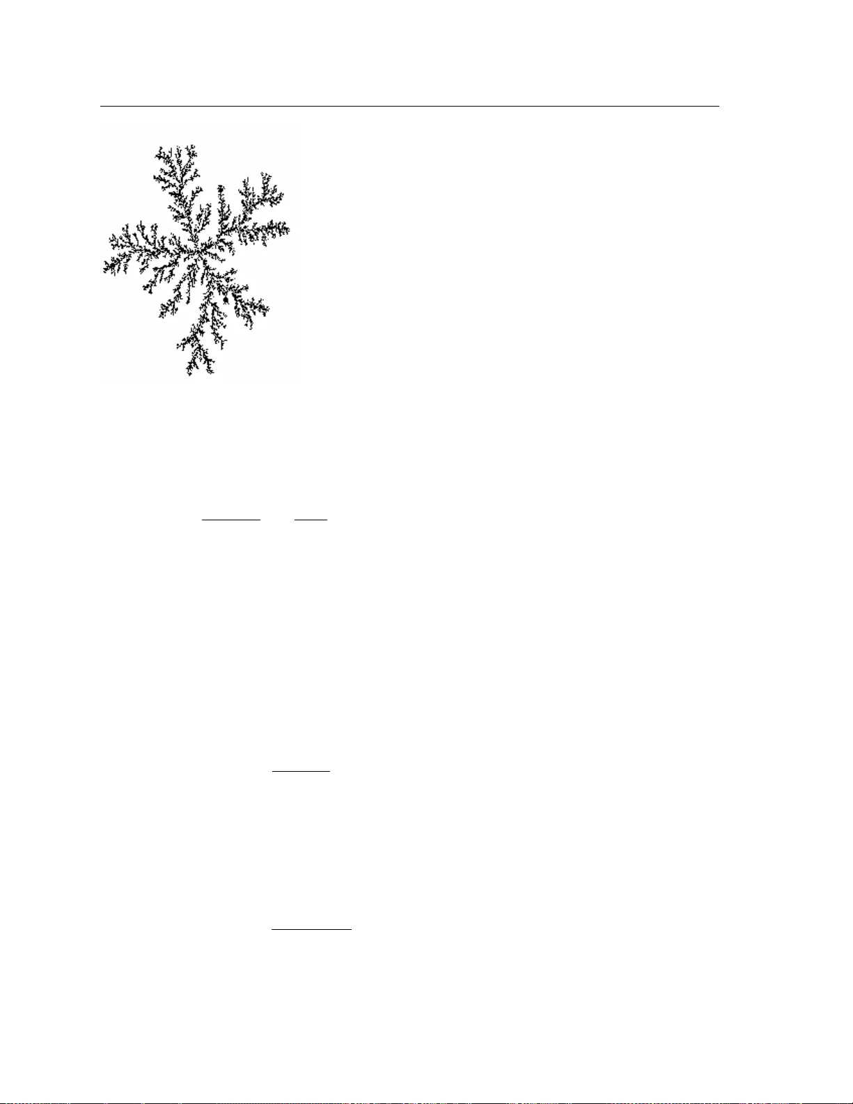
Random Matrices in 2D, Laplacian Gro wth and Op erator Theory Mark Mineev 1 , Mihai Putinar 2 and Razv an T eo dorescu 3 1 M.S. P365, Los Alamos National Lab oratory , Los Alamos, NM 87505 2 Mathematics Departmen t, UCSB, San ta Barbara, CA 93106 3 Theoretical Division and the Cen ter for Nonlinear Studies, Los Alamos, NM 87505 E-mail: mariner@lanl.gov , mputinar@math.ucsb.edu , razvan@lanl.gov Abstract. Since it w as ﬁrst applied to the study of n uclear in teractions b y Wigner and Dyson, almost 60 years ago, Random Matrix Theory (RMT) has developed into a ﬁeld of its o wn whithin applied mathematics, and is no w essential to many parts of theoretical physics, from condensed matter to high energy . The fundamental results obtained so far rely mostly on the theory of random matrices in one dimension (the dimensionalit y of the sp ectrum, or equilibrium probability density). In the last few y ears, this theory has b een extended to the case where the sp ectrum is tw o-dimensional, or ev en fractal, with dimensions b et ween 1 and 2. In this article, w e review these recen t dev elopmen ts and indicate some ph ysical problems where the theory can b e applied. P ACS n umbers: 05.30, 05.40, 05.45 Submitted to: J. Phys. A: Math. Gen. CONTENTS 2 Con tents 1 In tro duction 4 2 Random Matrix Theory in 1D 5 2.1 The symmetry group ensem bles and their physical realisations . . . . . . 5 2.2 Critical ensembles . . . . . . . . . . . . . . . . . . . . . . . . . . . . . . . 7 2.2.1 General formalism . . . . . . . . . . . . . . . . . . . . . . . . . . 7 2.2.2 Con tinuum limit and integrable equations . . . . . . . . . . . . . 8 2.2.3 Scaled limits of orthogonal p olynomials and equilibrium measures 9 3 Random Matrix Theory in higher dimensions 10 3.1 The Ginibre-Girko ensem ble . . . . . . . . . . . . . . . . . . . . . . . . . 10 3.2 Normal matrix ensembles . . . . . . . . . . . . . . . . . . . . . . . . . . . 11 3.3 Droplets of eigenv alues . . . . . . . . . . . . . . . . . . . . . . . . . . . . 12 3.4 Orthogonal p olynomials and distribution of eigenv alues . . . . . . . . . . 12 3.5 W av efunctions, recursions and integrable hierarc hies . . . . . . . . . . . . 13 3.5.1 Pseudo-diﬀeren tial op erators . . . . . . . . . . . . . . . . . . . . . 13 3.5.2 Lev el reductions . . . . . . . . . . . . . . . . . . . . . . . . . . . . 14 3.5.3 T au functions and Baker-Akhiezer function . . . . . . . . . . . . . 15 3.6 Equations for the w av e functions and the sp ectral curv e . . . . . . . . . . 16 3.6.1 Finite dimensional reductions . . . . . . . . . . . . . . . . . . . . 17 3.7 Sp ectral curv e . . . . . . . . . . . . . . . . . . . . . . . . . . . . . . . . . 18 3.7.1 Sc hw arz function . . . . . . . . . . . . . . . . . . . . . . . . . . . 20 3.7.2 The Schottky double . . . . . . . . . . . . . . . . . . . . . . . . . 20 3.7.3 Degeneration of the sp ectral curv e . . . . . . . . . . . . . . . . . . 22 3.7.4 Example: genus one curv e . . . . . . . . . . . . . . . . . . . . . . 23 3.8 Con tinuum limit and conformal maps . . . . . . . . . . . . . . . . . . . . 26 4 Laplacian Gro wth 27 4.1 In tro duction . . . . . . . . . . . . . . . . . . . . . . . . . . . . . . . . . . 27 4.2 Ph ysical bac kground . . . . . . . . . . . . . . . . . . . . . . . . . . . . . 28 4.3 Exact solutions . . . . . . . . . . . . . . . . . . . . . . . . . . . . . . . . 34 4.4 Mathematical structure of Laplacian growth . . . . . . . . . . . . . . . . 40 4.4.1 Conserv ation of harmonic moments . . . . . . . . . . . . . . . . . 40 4.4.2 LG and the In verse P otential Problem . . . . . . . . . . . . . . . 40 4.4.3 Laplacian growth in terms of the Sch w arz function . . . . . . . . 41 4.4.4 The corresp ondence of singularities . . . . . . . . . . . . . . . . . 42 4.4.5 A ﬁrst classiﬁcation of singularities . . . . . . . . . . . . . . . . . 42 4.4.6 Hydro dynamics of LG and the singularities of Sch w arz function . 43 4.4.7 V ariational formulation of Hele-Sha w dynamics . . . . . . . . . . 44 CONTENTS 3 5 Quadrature Domains 46 5.1 Quadrature domains for subharmonic functions . . . . . . . . . . . . . . 46 5.2 Quadrature domains for analytic functions . . . . . . . . . . . . . . . . . 49 5.3 Mark ov’s momen t problem . . . . . . . . . . . . . . . . . . . . . . . . . . 52 5.3.1 Marko v’s extremal problem and the phase shift . . . . . . . . . . 54 5.3.2 The reconstruction algorithm in one real v ariable . . . . . . . . . 57 5.4 The exp onen tial transform in tw o dimensions . . . . . . . . . . . . . . . . 60 5.5 Semi-normal op erators . . . . . . . . . . . . . . . . . . . . . . . . . . . . 62 5.5.1 Applications: Laplacian gro wth . . . . . . . . . . . . . . . . . . . 65 5.6 Linear analysis of quadrature domains . . . . . . . . . . . . . . . . . . . 66 5.7 Signed measures, instability , uniqueness . . . . . . . . . . . . . . . . . . . 70 6 Other ph ysical applications of the op erator theory form ulation 75 6.1 Cusps in Laplacian gro wth: P ainlev´ e equations . . . . . . . . . . . . . . . 75 6.1.1 Univ ersality in the scaling region at critical p oin ts – a conjecture . 75 6.1.2 Scaling at critical p oin ts of normal matrix ensembles . . . . . . . 76 6.1.3 Conclusions . . . . . . . . . . . . . . . . . . . . . . . . . . . . . . 79 6.2 Non-comm utative probabilit y theory and 2D quantum mo dels . . . . . . 79 6.2.1 Metal-insulator transition in t wo dimensions . . . . . . . . . . . . 79 6.2.2 Non-comm utative probabilit y theory and free random v ariables . 81 4 1. Introduction During the second half of last cen tury and con tinuing through the presen t, random matrix theory has gro wn from a sp ecial metho d of theoretical physics, mean t to appro ximate energy levels of complex n uclei [1, 2, 3, 4, 5, 6, 7], in to a v ast mathematical theory with many diﬀeren t application in physics, computer and electrical engineering. Simply describing all the developmen ts and metho ds curren tly emplo y ed in this context w ould result in a monography m uch more extensiv e than this review. Therefore, we will only brieﬂy mention topics whic h are themselves very in teresting, but lie b ey ond the scop e of this w ork. The applications of random matrix theory (RMT) in to ph ysics ha v e b een extended from the original sub ject, sp ectra of heavy n uclei, to descriptions of large N S U ( N ) gauge theory [8, 9], critical statistical mo dels in tw o dimensions [10, 11, 12] disordered electronic systems [13, 14, 15, 16, 17, 18], quantum c hromo-dynamics (QCD) [19, 20], to name only a few. Non-physics applications range from communication theory [21] to sto c hastic pro cesses out of equilibrium [22, 23] and ev en more exotic topics [24]. A n umber of important results, b oth at theoretical and applied lev els, w ere obtained from the connection betw een random matrices and orthogonal p olynomials, esp ecially in their w eighted limit [25, 26, 9, 27, 28]. These w orks explored the relationship b et w een the branc h cuts of spectral (Riemann) curv es of systems of diﬀ eren tial equations and the supp ort of limit measures for w eighted orthogonal p olynomials. Y et another interesting connection stemming from this approac h is with the general (matrix) version of the Riemann-Hilb ert problem with ﬁnite supp ort [29, 30]. In [31, 32], it w as show ed that such relationships also hold for the class of normal random matrices. Unlik e in previous works, for this ensemble, the supp ort of the equilibrium distribution for the eigenv alues of matrices in the inﬁnite-size limit, is tw o- dimensional, whic h allo ws to in terpret it as a growing cluster in the plane. Th us, a direct relation to the class of mo dels kno wn as Laplacian Growth (b oth in the deterministic and sto chastic form ulations), was deriv ed, with imp ortant consequences. In particular, this approac h allo w ed to study formation of singularities in mo dels of tw o-dimensional gro wth. Moreo ver, these results allow ed to deﬁne a prop er wa y of con tin uing the solution for singular Laplacian Gro wth, b eyond the critical p oint. F rom the p oin t of view of the dimensionalit y of the supp ort for random matrix eigen v alues, it is p ossible to distinguish b etw een 1-dimensional situations (whic h c haracterize 1 and 2-matrix mo dels), and 2-dimensional situations, lik e in the case of normal random matrix theory . In fact, v ery recen t results p oint to in termediate cases, where the supp ort is a set of dimensional b et ween 1 and 2. This situation is very similar to the description of disordered, interacting electrons in the plane, in the vicinity of the critical p oint whic h separates lo calized from de-lo calized b ehavior [15]. It is from the p ersp ectiv e of the dimensionalit y of supp ort for equilibrium measure that w e ha ve organized this review. The pap er is structured in the follo wing wa y: after a brief summary of the main 5 concepts in Section 2, w e explain the structure of normal random matrices in the limit of inﬁnite size, in Section 3. This allo ws to connect with planar gro wth mo dels, of whic h Laplacian (or harmonic) Growth is a main representativ e. The following tw o sections giv e a solid description of the ph ysical (Section 4) and mathematical (Section 5) structure of harmonic growth. The discretized (or quantized) v ersion of this problem is precisely given by normal random matrices, as we indicate in these sections. Next w e presen t a general sc heme for enco ding shade functions in the plane into linear data, speciﬁcally into a linear b ounded Hilb ert space op erator T with rank one self- comm utator rank[ T ∗ , T ] = 1. This line of research go es bac k to the p erturbation and scattering theory of symmetric op erators (M. G. Krein’s phase shift function) and to studies related to singular integral op erators with a Cauch y kernel t yp e singularity . Multiv ariate reﬁnements of the ”quantization sc heme” w e outline in Chapter 5 lie at the foundations of b oth cyclic (co)homology of op erator algebras and of free probabilit y theory . In view of the scop e and length of the present survey , w e conﬁne ourselv es to only outline the surprising link b etw een quadrature domains and suc h Hilb ert space ob jects. W e conclude with an application of the op erator formalism to the description of b oundary singular p oin ts that are c haracteristic to Laplacian gro wth evolution, and a brief ov erview of other related topics. 2. Random Matrix Theory in 1D 2.1. The symmetry gr oup ensembles and their physic al r e alisations F ollowing [33], we repro duce the standard in tro duction of the symmetry-groups ensemble of random matrices. The traditional ensembles (orthogonal, unitary and symplectic) w ere introduced mainly b ecause of their signiﬁcance with resp ect to symmetries of hamiltonian op erators in physical theories: time-rev ersal and rotational in v ariance corresp onds to the orthogonal ensem ble (whic h, for Gaussian measures, is naturally abbreviated GOE), while time-rev ersal alone and rotational in v ariance alone corresp ond to the symplectic and unitary ensembles, resp ectively (GSE and GUE for Gaussian measures). An inv ariant measure is deﬁned for eac h of these ensembles, in the form d e µ ( M ) ≡ P ( M ) dµ ( M ) ≡ Z − 1 e − T r[ W ( M )] dµ ( M ) , (1) where M is a matrix from the ensem ble, Z is a normalization factor (partition function), T r[ W ( M )] is inv ariant under the symmetries on the ensem ble, and dµ ( M ) is the appropriate ﬂat measure for that ensemble: Q i ≤ j dM ij for orthogonal, Q i ≤ j d Re M ij Q i 0 , (8) for which the deformation in not a simple rescaling. In this case, it is p ossible to consider a special limit n → ∞ , λ → ∞ , λ → nr c , where r c is a constant. As w e will see, for a sp eciﬁc v alue of r c , this limit yields a sp ecial asymptotic b eha vior of the orthonormal functions ψ n ( x ). How ever, ev en for the simplest, trivial monomial (a Gaussian), which yields the Hermite p olynomials, the asymptotic b eha vior of the orthogonal functions is non-trivial, in the sense that there are no known goo d approximations for the case r c = O (1). Generically , in this large n, λ limit, w e can ask where the w av efunction ψ n ( x ) will reac h its maximum v alue, in the saddle p oint appro ximation: max | x | ∂ x | ψ n ( x ) | = 0 , (9) giving ∂ x " n X i =1 log( x − ξ i ) − nr c + W ( x ) # = 0 , (10) so that − r c W 0 ( x ) = 2 n n X i =1 1 x − ξ i , (11) 2.2 Critical ensem bles 8 where ξ i , i = 1 , . . . , n are the ro ots of the n th p olynomial. Let ω ( z ) = 1 n n X i =1 1 ξ i − z , (12) m ultiply (11) by ( ξ i − z ) − 1 and sum ov er i , and obtain ω 2 ( z ) − r c W 0 ( z ) ω ( z ) = − r c n n X i =1 W 0 ( z ) − W 0 ( ξ i ) z − ξ i . (13) Equation (13) can b e solv ed in the large n limit b y assuming that the roots will b e distributed with densit y ρ ( ξ ) on some compact (p ossibly disconnected) set I ⊂ R . Deﬁning R ( z ) = − 4 r c Z I W 0 ( z ) − W 0 ( ξ ) z − ξ ρ ( ξ ) dξ , (14) w e obtain ω 2 ( z ) − r c W 0 ( z ) ω ( z ) +  r c 2  2 R ( z ) = 0 . (15) The prop er solution of (13) (considering the b ehavior at ∞ of the function ω ( z )), is ω ( z ) = r c 2 h W 0 ( z ) + p ( W 0 ( z )) 2 − R ( z ) i , (16) and (since the function ω ( z ) is the Cauch y transform of the densit y ρ ( x )), it gives us the asymptotic distribution of zeros as ρ ( x ) = 1 2 π i [ ω ( x + i 0) − ω ( x − i 0)] . (17) Finally , to obtain the asymptotic form of wa v e functions ψ n ( x ), we can write n − 1 log ψ n ( x ) → Z ρ ( ξ ) log( x − ξ ) dξ − r c 2 + W ( x ) . (18) 2.2.2. Continuum limit and inte gr able e quations There are t w o related problems for the large n limit of deformed ensembles describ ed in the previous section. The ﬁrst is determination of the supp ort of zeros I ; the second is the scaling b eha vior of the orthogonal functions ψ n ( x ). In general, the limiting supp ort I ma y consist of several disconnected segments I k , I = ∪ k = d k =1 I k . In the simplest case, it is just one in terv al I = [ a, b ] ⊂ R . In this section we indicate how to determine this supp ort as w ell as the densit y ρ ( x ), and what this yields for the orthogonal functions. Let the function W ( x ) b e a p olynomial of even degree d . F rom (14) w e see that R ( z ) is a p olynomial of degree d − 2, and therefore solution (16) has generically 2( d − 1) branc h p oin ts. Thus, the function ω ( z ) typically has d − 1 branc h cuts, whic h constitute the disconnected supp ort of distribution ρ ( z ). W e are in terested in a sp ecial case, when d − 2 of these cuts degenerate in to double p oin ts, and there is a single in terv al [ a, b ] whic h is the supp ort of ρ ( z ). This special case is called cr itical and it pro vides new asymptotic limits for the orthogonal functions. W e will also refer to this solution as the “single-cut” solution. 2.2 Critical ensem bles 9 F rom the equation ω ( x + i 0) − ω ( x − i 0) = r c W 0 ( x ) , (19) w e obtain for the single-cut solution ω ( z ) = − r c p ( z − a )( z − b ) 2 π Z b a W 0 ( ξ ) p ( b − ξ )( ξ − a ) dξ ξ − z . The large | z | b ehavior of this function is known from the con tin uum limit of (12), and it implies the absence of regular terms in the Lauren t expansion: ω ( z ) = − 1 z + O ( z − 2 ) , (20) so that we imp ose the conditions 0 = Z b a W 0 ( ξ ) p ( b − ξ )( ξ − a ) dξ , (21) 2 π = − r c Z b a ξ W 0 ( ξ ) p ( b − ξ )( ξ − a ) dξ . (22) Gaussian me asur e and the Hermite p olynomials Let d = 2 and − W ( x ) = ax 2 , a > 0. Then conditions (21,22) giv e a symmetric supp ort [ − b, b ] where b 2 = 2 / ( ar c ). More generally , using the saddle p oin t equation for | ψ n ( x ) | at x = a, b and (18), we conclude that log ψ n ( b + ζ ) n = C b − r c 2 Z ζ 0 p [ W 0 ( b + η )] 2 − Rdη (23) Since the integrand b eha ves lik e η d − 3 / 2 , we obtain ψ n ( b + ζ ) = ψ n ( b ) exp  − nr c 2 d − 1 ζ d − 1 / 2  . (24) W e immediately conclude that for d = 2 (Hermite p olynomials), the asymptotic b eha vior is giv en b y the Airy function, exp z 3 / 2 . The full scaling is ac hieved b y considering the region around the end-p oin t b , of order ζ = O ( n − 2 / (2 d − 1) ).Then we obtain ψ n ( b + ˜ ζ n − 2 2 d − 1 ) ∼ exp  − r c 2 d − 1 ˜ ζ d − 1 / 2  . (25) 2.2.3. Sc ale d limits of ortho gonal p olynomials and e quilibrium me asur es The distribution of eigen v alues in vestigated in the previous sections illustrates the general approac h dev elop ed b y Saﬀ and T otik [26] for holomorphic p olynomials orthogonal on curv es in the complex plane. W e sketc h here the more general result b ecause of its relev ance to the main topic of this review. Giv en a set Σ ∈ C and a properly-deﬁned measure on it w ( z ) = e − Q ( z ) , w e construct the holomorphic orthogonal p olynomials P n ( z ), with resp ect to w . W e then p ose the question of ﬁnding the “extremal” measure (its supp ort S w and density µ w ), such that 10 the F -functional F ( K ) ≡ log cap( K ) − R Qdω K , with cap( K ) and ω K the capacit y , resp ectiv ely the equilibrium measure of the set K , is maximized b y S w . F urthermore, µ w satisﬁes energy and capacit y constrain ts on S w . The remark able fact noticed in [26] is that if the extremal v alue F ( S w ) is appro ximated b y the weigh ted monic polynomials ˜ P n ( z ) as ( || w n ˜ P n || ∗ Σ ) 1 /n → exp( − F w ) (where we use the w eak star norm), then the asymptotic zero distribution of ˜ P n giv es the supp ort S w . Hence, (17) ma y b e in terpreted as giving b oth the support of the extremal measure (lab eled ρ in this formula), as well as its actual density . The extremal measure has the physical in terpretation of t he “smallest” equilibrium measure whic h giv es a prescrib ed logarithmic p otential at inﬁnity . According to the concept of “sw eeping” (or “balay age”, see [26]), the extremal measure is obtained as a limit of the process, under the constrain ts imp osed on the total mass and energy of the measure. As we hav e shown in this c hapter, for the case of 1D measures, this extreme case is given b y weigh ted limits of orthogonal p olynomials. 3. Random Matrix Theory in higher dimensions In this chapter, we sho w how to generalize the concepts of equilibrium measure, extremal measure, and their relations to orthogonal p olynomials and ensem bles of random matrices, in the case of t w o-dimensional supp ort. The applications of this theory to planar growth processes will b e discussed in the following t wo c hapters. 3.1. The Ginibr e-Girko ensemble W e begin with a brief discussion on the oldest and simplest ensem ble of random matrices with planar supp ort. The ensem ble of complex, N × N random matrices with iden tical, indep enden t, zero-mean Gaussian-distributed en tries, was ﬁrst studied b y J. Ginibre in 1965 [35], and then it w as generalized for non-zero mean Gaussian b y Girk o in 1985 [36]. Consider N × N random matrices with eigenv alues z k ∈ C , and joint p.d.f. dP N ∼ Y 1 ≤ ij ( z i − z j ) is the V andermonde determinant, and τ N = 1 N ! Z | ∆ N ( z ) | 2 N Y j =1 e 1 ~ W ( z j , ¯ z j ) d 2 z j (29) is a normalization factor, the partition function of the matrix mo del (a τ -function). A particularly imp ortant sp ecial case arises if the p oten tial W has the form W = −| z | 2 + V ( z ) + V ( z ) , (30) where V ( z ) is a holomorphic function in a domain which includes the supp ort of eigen v alues (see also a commen t in the end of Section 3.4 ab out a prop er deﬁnition of the ensem ble with this potential). In this case, a normal matrix ensem ble gives the same distribution as a general complex matrix ensem ble. A general complex matrix can b e decomp osed as M = U ( Z + R ) U † , where U and Z are unitary and diagonal matrices, resp ectiv ely , and R is an upp er triangular matrix. The distribution (28) holds for the elemen ts of the diagonal matrix Z whic h are eigenv alues of M . Here w e mostly focus on the sp ecial p otential (30), and also assume that the ﬁeld A ( z ) = ∂ z V ( z ) (31) is a globally deﬁned meromorphic function. 3.3 Droplets of eigen v alues 12 Figure 1. A supp ort of eigenv alues consisting of four disconnected components (left). The distribution of eigen v alues for p oten tial V ( z ) = − α log (1 − z /β ) − γ z . (right) 3.3. Dr oplets of eigenvalues In the large N limit ( ~ → 0, N ~ ﬁxed), the eigenv alues of matrices from the ensem ble densely o ccupy a connected domain D in the complex plane, or, in general, several disconnected domains. This set (called the supp ort of eigenv alues) has sharp edges (Figure 1). W e refer to the connected comp onen ts D α of the domain D as dr oplets . F or algebraic domains (the deﬁnition follo ws) the eigenv alues are distributed with the densit y ρ = − 1 4 π ∆ W , where ∆ = 4 ∂ z ∂ ¯ z is the 2-D Laplace op erator [31]. F or the p oten tial (30) the densit y is uniform. The shap e of the supp ort of eigenv alues is the main sub ject of this chapter. F or example, if the p oten tial is Gaussian [35], A ( z ) = 2 t 2 z , (32) the domain is an ellipse. If A has one simple p ole, A ( z ) = − α z − β − γ (33) the droplet (under certain conditions discussed below) has the proﬁle of an aircraft wing giv en b y the Jouko wsky map (Figure 1). If A has one double p ole (sa y , at inﬁnity), A ( z ) = 3 t 3 z 2 , (34) the droplet is a h yp otro choid. If A has t wo or more simple p oles, there may b e more than one droplet. This supp ort and densit y represent the equilibrium solution to an electrostatic problem, as w e will indicate in a later section. 3.4. Ortho gonal p olynomials and distribution of eigenvalues Deﬁne the exact N -particle w av e function (up to a phase), by Ψ N ( z 1 , . . . , z N ) = 1 √ N ! τ N ∆ N ( z ) e P N j =1 1 2 ~ W ( z j , ¯ z j ) . (35) 3.5 W a vefunctions, recursions and integrable hierarchies 13 The joint probabilit y distribution (28) is then equal to | Ψ( z 1 , . . . , z N ) | 2 . Let the num b er of eigenv alues (particles) increase while the p oten tial stays ﬁxed. If the supp ort of eigen v alues is simply-connected, its area grows as ~ N . One can describe the evolution of the domain through the densit y of particles ρ N ( z ) = N Z | Ψ N ( z , z 1 , z 2 , . . . , z N − 1 ) | 2 d 2 z 1 . . . d 2 z N − 1 , (36) where Ψ N is given b y (35). W e introduce a set of orthonormal one-particle functions on the complex plane as matrix elements of transitions b etw een N and ( N + 1)-particle states: ψ N ( z ) √ N + 1 = Z Ψ N +1 ( z , z 1 , z 2 , . . . , z N )Ψ N ( z 1 , z 2 , . . . , z N ) d 2 z 1 . . . d 2 z N (37) Then the rate of the density c hange is ρ N +1 ( z ) − ρ N ( z ) = | ψ N ( z ) | 2 . (38) The proof of this form ula is based on the rep resen tation of the ψ n through holomorphic biorthogonal p olynomials P n ( z ). Up to a phase ψ n ( z ) = e 1 2 ~ W ( z , ¯ z ) P n ( z ) , P n ( z ) = r τ n τ n +1 z n + . . . (39) The p olynomials P n ( z ) are biorthogonal on the complex plane with the w eight e W/ ~ : Z e W/ ~ P n ( z ) P m ( z ) d 2 z = δ mn . (40) The pro of of these form ulae is standard in the theory of orthogonal p olynomials. Extension to the biorthogonal case adds no diﬃculties. W e note that, with the choice of p otential (30), the in tegral represen tation (40) has only a formal meaning, since the in tegral div erges unless the p oten tial is Gaussian. A prop er deﬁnition of the w av e functions go es through recursiv e relations (53, 54) whic h follo w from the integral represen tation. The same commen t applies to the τ -function (29). The wa ve function is not normalized everywhere in the complex plane. It may div erge at the p oles of the v ector p otential ﬁeld. 3.5. Wavefunctions, r e cursions and inte gr able hier ar chies In order to illustrate the mathematical connection betw een this theory and equiv alen t form ulations whic h w e presen t in Chapter 5, it is necessary to mak e a digression through the formalism of inﬁnite, integrable hierarchies. In particular, w e choose the case of the Kadom tsev-Petviash vilii (KP) hierarc hy , and follow the notations in [42]. 3.5.1. Pseudo-diﬀer ential op er ators W e denote by A the algebra constructed from diﬀeren tial polynomials of the t yp e P = ∂ n + u n − 2 ∂ n − 2 + . . . + u 1 ∂ + u 0 , where ∂ = ∂ /∂ z is a diﬀeren tial symbol with resp ect to some (complex) v ariable z , and u 0 , u 1 , . . . , u n − 2 (note: u n − 1 can b e alwa ys set to zero) are generically smo oth functions in z and (if 3.5 W a vefunctions, recursions and integrable hierarchies 14 necessary) other v ariables t 1 , t 2 , . . . . On this algebra, w e deﬁne the ring of pseudo- diﬀeren tial op erators R , consisting of (formal) op erators deﬁned b y the inﬁnite series L = n X −∞ c k ∂ k , ∂ − 1 ≡ Z dz , (41) where co eﬃcients are again smooth functions, and the negativ e pow ers in the expansions con tain integ r al op erators. F or an y suc h op erator, we denote b y L + the purely diﬀeren tial part and by L − the remainder of the series: L + ≡ n X 0 c k ∂ k , L = L + + L − . (42) Let L = ∂ + u 0 ∂ − 1 + u 1 ∂ − 2 + . . . (43) b e a pseudo-diﬀeren tial op erator such that L + = ∂ . Then, introducing the inﬁnite set of times t = t 1 , t 2 , . . . , suc h that all co eﬃcien ts u k , c k ab o v e are generically functions of t , the KP hierarc hy has the form ∂ L ∂ t k = [ L k + , L ] , k = 1 , 2 , . . . (44) More explicitly , w e note that the hierarch y consists of the diﬀerential equations satisﬁed b y the c o eﬃcients of the op erator L . As a consequence of the compatibility of all the equations in the hierarc hy , w e hav e the zer o-curvatur e e quations [ ∂ t k − L k + , ∂ t p − L p + ] = 0 , ∀ t k , t p . (45) 3.5.2. L evel r e ductions The KP hierarc hy con tains man y other kno wn integrable hierarc hies, particularly the KdV hierarch y , as reductions to a certain l ev el n in the hierarc hy . F or example, assume that the op erator L satisﬁes the constraint L 2 − = 0 , (46) i.e. it is the square ro ot of a diﬀer ential op erator L of order 2: L = L 1 / 2 , L = ∂ 2 + 2 u 0 . (47) Then it follows that for all even p ow ers n = 2 m , L n + = L n , so that [ L n + , L ] = 0, so there is no dep endence on the even times t 2 , t 4 , . . . . This sub-hierarch y is called l ev el − 2 KdV, because the ﬁrst non-trivial zero-curv ature equation of the hierarc h y is the famous Kortew eg-de V ries equation: L 3 + ≡ P = ∂ 3 + 3 2 [ u 0 ∂ + ∂ u 0 ] , ∂ L ∂ t 3 = [ P , L ] ⇒ u t 3 = 6 uu z + u z z z , (48) where we ha v e used u 0 = u for clarity . This form ulation of the KdV equation mak es use of the notion of Lax pair L, P , whic h is central to the inverse sc attering metho d for solving nonlinear integrable 3.5 W a vefunctions, recursions and integrable hierarchies 15 diﬀeren tial equations The idea is quite physical: assume that the op erators L, P act on a wa v efunction ψ ( x, t ) suc h that Lψ = λψ , ∂ ψ ∂ t = P ψ , (49) where eigen v alues λ form the sp ectrum of L . Then applying the Lax pair equation to the eigenv alue equation, we obtain ∂ λ/∂ t = 0, i.e. the evolution under these equations lea ves the sp ectrum in v ariant. This allows to construct the initial state from the ﬁnal state, hence the in verse scattering app ellation. 3.5.3. T au functions and Baker-Akhiezer function A t the lev el of systems of PDE, the τ − function and the Bak er-Akhiezer function are introduced, by analogy with the Lax par formulation indicated ab o ve, in the following w ay: Baker-A khiezer function Consider the function ψ ( z , t 1 , t 2 , . . . ) satisfying L ψ = z ψ , ∂ ψ ∂ t k = L k + ψ , ∀ k ≥ 1 . (50) This is the Bak er-Akhiezer function of the KP hierarch y . F undamental pr op erty of the Baker-A khiezer function Let φ = 1 + P ∞ 0 k i ∂ − i − 1 b e the “dressing” op erator deﬁned such that L = φ∂ φ − 1 . Also, introduce the function g ( z , t 1 , . . . ) = exp[ P ∞ 1 t k z k ]. Then the Baker-Akhiezer function satisﬁes: ψ = ˆ k ( z ) g ( z , t 1 , . . . ) , ˆ k ( z ) = 1 + ∞ X 0 k i z − i − 1 , where ˆ k is the “scalar” analog of the dressing op erator φ . T au function Using the notation introduced ab ov e, we ha ve the follo wing prop ert y: There exists a function τ ( z , t 1 , . . . ) suc h that ψ ( z , t 1 , . . . ) = g · τ ( z , t 1 − 1 z , t 2 − 1 2 z 2 , . . . ) τ ( z , t 1 , t 2 , . . . ) = g · exp h P ∞ 1 − 1 kz k ∂ ∂ t k i τ ( z , t 1 , . . . ) τ ( z , t 1 , . . . ) No w let us consider the generalized ov erlap function ψ N ( z , ¯ w ) = τ − 1 N Z Ψ N +1 ( z , z 1 , z 2 , . . . , z N )Ψ N +1 ( w , z 1 , z 2 , . . . , z N ) d 2 z 1 . . . d 2 z N , and expand for | z | , | w | → ∞ . W e obtain ψ N ( z , ¯ w ) = ( z ¯ w ) N τ N exp  X − 1 z k ¯ w p ∂ ∂ a kp  τ N , (51) where a kp is the corresp onding in terior bi-harmonic moment. Therefore, w e ma y regard the τ -function and the scaled w a vefunction introduced earlier as canonical ob jects describing an in tegrable hierarch y . This fact will b e illustrated in more detail in the next section. 3.6 Equations for the w av e functions and the sp ectral curve 16 3.6. Equations for the wave functions and the sp e ctr al curve In this section we specify the p oten tial to b e of the form (30). It is conv enien t to mo dify the exp onential factor of the wa v e function. Namely , w e deﬁne ψ n ( z ) = e − | z | 2 2 ~ + 1 ~ V ( z ) P n ( z ) , and χ n ( z ) = e 1 ~ V ( z ) P n ( z ) , (52) where the holomorphic functions χ n ( z ) are orthonormal in the complex plane with the w eight e −| z | 2 / ~ . Like traditional orthogonal polynomials, the biorthogonal p olynomials P n (and the corresp onding wa v e functions) ob ey a set of diﬀerential equations with resp ect to the argumen t z , and recurrence relations with resp ect to the degree n . Similar equations for tw o-matrix mo dels are discussed in n umerous pap ers (see, e.g., [43]). W e in tro duce the L -op erator (the Lax operator) as m ultiplication b y z in the basis χ n : L nm χ m ( z ) = z χ n ( z ) (53) (summation ov er repeated indices is implied). Obviously , L is a low er triangular matrix with one adjacent upper diagonal, L nm = 0 as m > n + 1. Similarly , the diﬀerentiation ∂ z is represen ted b y an upp er triangular matrix with one adjacent lo w er diagonal. In tegrating b y parts the matrix elemen ts of the ∂ z , one ﬁnds: ( L † ) nm χ m = ~ ∂ z χ n , (54) where L † is the Hermitian conjugate op erator. The matrix elements of L † are ( L † ) nm = ¯ L mn = A ( L nm ) + R e 1 ~ W ¯ P m ( ¯ z ) ∂ z P n ( z ) d 2 z , where the last term is a lo wer triangular matrix. The latter can b e written through negativ e p o wers of the Lax op erator. W riting ∂ z log P n ( z ) = n z + P k> 1 v k ( n ) z − k , one represen ts L † in the form L † = A ( L ) + ( ~ n ) L − 1 + X k> 1 v ( k ) L − k , (55) where v ( k ) and ( ~ n ) are diagonal matrices with elements v ( k ) n and ( ~ n ). The co eﬃcients v ( k ) n are determined by the condition that lo wer triangular matrix elemen ts of A ( L nm ) are cancelled. In order to emphasize the structure of the op erator L , w e write it in the basis of the shift op erator ‡ ˆ w such that ˆ w f n = f n +1 ˆ w for any sequence f n . Acting on the wa ve function, we ha v e: ˆ w χ n = χ n +1 . In the n -representation, the op erators L , L † acquire the form L = r n ˆ w + X k ≥ 0 u ( k ) n ˆ w − k , L † = ˆ w − 1 r n + X k ≥ 0 ˆ w k ¯ u ( k ) n . (56) ‡ The shift op erator ˆ w has no inv erse. Belo w ˆ w − 1 is understo o d as a shift to the left deﬁned as ˆ w − 1 ˆ w = 1. Same is applied to the op erator L − 1 . T o av oid a p ossible confusion, we emphasize that although χ n is a righ t-hand eigen v ector of L , it is not a righ t-hand eigen v ec tor of L − 1 . 3.6 Equations for the w av e functions and the sp ectral curve 17 Clearly , acting on χ n , we ha v e the commutation relation (“the string equation”) [ L, L † ] = ~ . (57) This is the compatibilit y condition of Eqs. (53) and (54). Equations (56) and (57) completely determine the co eﬃcients v ( k ) n , r n and u ( k ) n . The ﬁrst one connects the co eﬃcients to the parameters of the p oten tial. The second equation is used to determine ho w the co eﬃcien ts v ( k ) n , r n and u ( k ) n ev olve with n . In particular, the diagonal part of it reads n ~ = r 2 n − X k ≥ 1 k X p =1 | u ( k ) n + p | 2 . (58) Moreo ver, we note that all the coeﬃcients can be e xpressed through the τ -function (29) and its deriv ativ es with resp ect to parameters of the potential. This representation is particularly simple for r n : r 2 n = τ n τ − 2 n +1 τ n +2 . 3.6.1. Finite dimensional r e ductions If the v ector p otential A ( z ) is a rational function, the co eﬃcien ts u ( k ) n are not all indep endent. The num b er of indep endent co eﬃcien ts equals the n um b er of indep endent parameters of the p oten tial. F or example, if the holomorphic part of the p oten tial, V ( z ), is a p olynomial of degree d , the series (56) are truncated at k = d − 1. In this case the semi-inﬁnite system of linear equations (54) and the recurrence relations (53) can b e cast in the form of a set of ﬁnite dimensional equations whose co eﬃcien ts are rational functions of z , one system for every n > 0. The system of diﬀerential equations generalizes the Cristoﬀel-Daurb oux second order diﬀerential equation v alid for orthogonal p olynomials. This fact has been observed in recent pap ers [44, 45] for biorthogonal p olynomials emerging in the Hermitian t w o-matrix mo del with a p olynomial potential. It is applicable to our case (holomorphic biorthogonal p olynomials) as well. In a more general case, when A ( z ) is a general rational function with d − 1 p oles (coun ting m ultiplicities), the series (56) is not truncated. How ever, L can b e represen ted as a “ratio”, L = K − 1 1 K 2 = M 2 M − 1 1 , (59) where the op erators K 1 , 2 , M 1 , 2 are p olynomials in ˆ w : K 1 = ˆ w d − 1 + d − 2 X j =0 A ( j ) n ˆ w j , K 2 = r n + d − 1 ˆ w d + d − 1 X j =0 B ( j ) n ˆ w j (60) M 1 = ˆ w d − 1 + d − 2 X j =0 C ( j ) n ˆ w j , M 2 = r n ˆ w d + d − 1 X j =0 D ( j ) n ˆ w j (61) These op erators ob ey the relation K 1 M 2 = K 2 M 1 . (62) 3.7 Sp ectral curve 18 It can b e pro v en that the pair of op erators M 1 , 2 is uniquely determined by K 1 , 2 and vice v ersa. W e note that the reduction (59) is a diﬀerence analog of t he “rational” reductions of the Kadomtsev-P etviash vili integrable hierarc h y considered in [46]. The linear problems (53), (54) acquire the form ( K 2 χ ) n = z ( K 1 χ ) n , ( M † 2 χ ) n = ~ ∂ z ( M † 1 χ ) n . (63) These equations are of ﬁnite or der (namely , of order d ), i.e., they connect v alues of χ n on d + 1 subsequen t sites of the lattice. The semi-inﬁnite set { χ 0 , χ 1 , . . . } is then a “bundle” of d -dimensional v ectors χ ( n ) = ( χ n , χ n +1 , . . . , χ n + d − 1 ) t (the index t means transp osition, so χ is a column vector). The dimension of the vector is the n um b er of p oles of A ( z ) plus one. Each v ector ob eys a closed d -dimensional linear diﬀeren tial equation ~ ∂ z χ ( n ) = L n ( z ) χ ( n ) , (64) where the d × d matrix L n is a “pro jection” of the op erator L † on to the n -th d -dimensional space. Matrix elements of the L n are rational functions of z having the same p oles as A ( z ) and also a p ole at the point A ( ∞ ). (If A ( z ) is a p olynomial, all these p oles accum ulate to a multiple p ole at inﬁnity). W e brieﬂy describ e the pro cedure of constructing the ﬁnite dimensional matrix diﬀeren tial equation. W e use the ﬁrst linear problem in (63) to represen t the shift op erator as a d × d matrix W n ( z ) with z -dep endent co eﬃcien ts: W n ( z ) χ ( n ) = χ ( n + 1) . (65) This is nothing else than rewriting the scalar linear problem in the matrix form. Then the matrix W n ( z ) is to b e substituted into the second equation of (63) to determine L n ( z ) (examples follo w). The en tries of W n ( z ) and L n ( z ) obey the Sc hlesinger equation, whic h follo ws from compatibility of (64) and (65): ~ ∂ z W n = L n +1 W n − W n L n . (66) This pro cedure has b een realized explicitly for p olynomial p otentials in recent pap ers [44, 45]. W e will work it out in detail for our three examples: χ ( n ) = ( χ n , χ n +1 ) t for the ellipse (32) and the aircraft wing (33) and χ ( n ) = ( χ n , χ n +1 , χ n +2 ) t for the h yp otro c hoid (34). 3.7. Sp e ctr al curve According to the general theory of linear diﬀeren tial equations, the semiclassical (WKB) asymptotics of solutions to Eq. (64), as ~ → 0, is found b y solving the eigenv alue problem for the matrix L n ( z ) [47]. More precisely , the basic ob ject of the WKB approac h is the sp ectral curv e [47] of the matrix L n , whic h is deﬁned, for every in teger n > 0, by the secular equation det( L n ( z ) − ˜ z ) = 0 (here ˜ z means ˜ z · 1 , where 1 is the unit d × d 3.7 Sp ectral curve 19 matrix). It is clear that the left hand side of the secular equation is a p olynomial in ˜ z of degree d . W e deﬁne the sp ectral curve b y an equiv alen t equation f n ( z , ˜ z ) = a ( z ) det( L n ( z ) − ˜ z ) = 0 , (67) where the factor a ( z ) is added to mak e f n ( z , ˜ z ) a p olynomial in z as well. The factor a ( z ) then has zeros at the points where p oles of the matrix function L ( z ) are lo cated. It do es not depend on n . W e will so on see that the degree of the p olynomial a ( z ) is equal to d . Assume that all poles of A ( z ) are simple, then zeros of the a ( z ) are just the d − 1 p oles of A ( z ) and another simple zero at the p oin t A ( ∞ ). Therefore, we conclude that the matrix L n ( z ) is rather sp ecial. F or a general d × d matrix function with the same d p oles, the factor a ( z ) would be of degree d 2 . Note that the matrix L n ( z ) − ¯ z en ters the diﬀeren tial equation ~ ∂ z | ψ ( n ) | 2 = ¯ ψ ( n )( L n ( z ) − ¯ z ) ψ ( n ) (68) for the squared amplitude | ψ ( n ) | 2 = ψ † ( n ) ψ ( n ) = e − | z | 2 ~ | χ ( n ) | 2 of the vectors ψ ( n ) built from the orthonormal w av e functions (39). The equation of the curv e can b e in terpreted as a “resultant” of the non- comm utative p olynomials K 2 − z K 1 and M † 2 − ˜ z M † 1 (cf. [44]). Indeed, the p oint ( z , ˜ z ) b elongs to the curv e if and only if the linear system      ( K 2 c ) k = z ( K 1 c ) k n − d ≤ k ≤ n − 1 ( M † 2 c ) k = ˜ z ( M † 1 c ) k n ≤ k ≤ n + d − 1 (69) has non-trivial solutions. The system contains 2 d equations for 2 d v ariables c n − d , . . . , c n + d − 1 . V anishing of the 2 d × 2 d determinan t yields the equation of the sp ectral curve. Below w e use this metho d to ﬁnd the equation of the curve in the examples. It app ears to b e muc h easier than the determination of the matrix L n ( z ). The spectral curv e (67) p ossesses an imp ortan t prop ert y: it admits an an tiholomorphic in v olution. In the co ordinates z , ˜ z the inv olution reads ( z , ˜ z ) 7→ ( ˜ z , ¯ z ). This simply means that the secular equation det( ¯ L n ( ˜ z ) − z ) = 0 for the matrix ¯ L n ( ˜ z ) ≡ L n ( ˜ z ) deﬁnes the same curv e. Therefore, the p olynomial f n tak es real v alues for ˜ z = ¯ z : f n ( z , ¯ z ) = f n ( z , ¯ z ) . (70) P oints of the real section of the curve ( ˜ z = ¯ z ) are ﬁxed p oints of the in v olution. The curve (67) w as discussed in recent papers [44, 45] in the context of Hermitian t wo-matrix mo dels with polynomial potentials. The dual realizations of the curv e p oin ted out in [44] corresp ond to the antiholomorphic inv olution in our case. The in volution can b e prov en along the lines of these works. The pro of is rather tec hnical and w e omit it, restricting ourselves to the examples b elo w. W e simply note that the in volution relies on the fact that the squared mo dulus of the wa v e function is real. W e will give a concrete example for the construction of the sp ectral curv e, after a brief but necessary detour through the con tinuum limit of this problem. 3.7 Sp ectral curve 20 3.7.1. Schwarz function The p olynomial f n ( z , ¯ z ) can b e factorized in tw o wa ys: f n ( z , ¯ z ) = a ( z )( ¯ z − S (1) n ( z )) . . . ( ¯ z − S ( d ) n ( z )) , (71) where S ( i ) n ( z ) are eigenv alues of the matrix L n ( z ), or f n ( z , ¯ z ) = a ( z )( z − ¯ S (1) n ( ¯ z )) . . . ( z − ¯ S ( d ) n ( ¯ z )) , (72) where ¯ S ( i ) n ( ¯ z ) are eigen v alues of the matrix ¯ L n ( ¯ z ). One may understand them as diﬀerent branc hes of a multiv alued function S ( z ) (resp ectively , ¯ S ( z )) on the plane (here we do not indicate the dependence on n , for simplicit y of the notation). It then follo ws that S ( z ) and ¯ S ( z ) are m utually inv erse functions: ¯ S ( S ( z )) = z . (73) An algebraic function with this prop ert y is called the Schwarz function . By the equation f ( z , S ( z )) = 0, it deﬁnes a complex curve with an antiholomorphic inv olution. An upp er bound for gen us of this curve is g = ( d − 1) 2 , where d is the n umber of branches of the Sch w arz function. The real section of this curve is a set of all ﬁxed p oints of the in volution. It consists of a num b er of contours on the plane (and p ossibly a n um b er of isolated p oin ts, if the curve is not smo oth). The structure of this set is known to b e complicated. Dep ending on co eﬃcien ts of the p olynomial, the num b er of disconnected con tours in the real section may v ary from 0 to g + 1. If the contours divide the complex curv e in to t wo disconnected “halv es”, or sides (related b y the in v olution), then the curv e can b e realized as the Schottky double [48] of one of these sides. Eac h side is a Riemann surface with a b oundary . Let us come bac k to equation (64). It has d indep enden t solutions. They are functions on the sp ectral curv e. One of them is a physical solution corresp onding to biorthogonal p olynomials. The physical solution deﬁnes the “ph ysical sheet” of the curv e. The Sc h warz function on the physical sheet is a particular ro ot, say S (1) n ( z ), of the p olynomial f n ( z , ˜ z ) (see (71)). It follo ws from (55) that this ro ot is selected by the requiremen t that it has the same p oles and residues as the p otential A . 3.7.2. The Schottky double The Sch wa rz function describ es more than just the b oundary of clusters of eigenv alues. T ogether with other sheets it deﬁnes a Riemann surface. If the potential A ( z ) is meromorphic, the Sch warz function is an algebraic function. It satisﬁes a p olynomial equation f ( z , S ( z )) = 0. The function f ( z , ˜ z ), where z and ˜ z are treated as t wo indep endent complex argumen ts, deﬁnes a Riemann surface with antiholomorphic inv olution (70). If the in volution divides the surface into t wo disconnected parts, as explained ab ov e, the Riemann surface is the Schottky double [48] of one of these parts. There are t wo complementary wa ys to describ e this surface. One is through the algebraic cov ering (71, 72). Among d sheets we distinguish a physic al sheet. The ph ysical sheet is selected b y the condition that the diﬀeren tial S ( z ) dz has the same p oles and residues as the diﬀerential of the p otential A ( z ) dz . It ma y happ en that the condition 3.7 Sp ectral curve 21 ! ! Figure 2. The Schottky double. A Riemann surface with b oundaries along the droplets (a fron t side) is glued to its mirror image (a back side). ¯ z = S ( i ) ( z ) deﬁnes a planar curv e (or sev eral curv es, or a set of isolated points) for branc hes other than the ph ysical one. W e refer to the in terior of these planar curv es as virtual (or unphysical) droplets situated on sheets other than physical. Another w ay emphasizes the antiholomorphic in v olution. Consider a meromorphic function h ( z ) deﬁned on a Riemann surface with b oundaries. W e call this surface the fron t side. The Sch warz reﬂection principle extends any meromorphic function on the fron t side to a meromorphic function on the Riemann surface without b oundaries. This is done b y adding another copy of the Riemann surface with b oundaries (a back side), glued to the fron t side along the boundaries, Figure 2. The v alue of the function h on the mirror p oint on the back side is h ( S ( z )). The copies are glued along the b oundaries: h ( z ) = h ( S ( z )) if the p oint z belongs to the b oundary . The same extension rule applies to diﬀerentials. Ha ving a meromorphic diﬀeren tial h ( z ) dz on the front side, one extends it to a meromorphic diﬀerential h ( S ( z )) dS ( z ) on the back side. This deﬁnition can be applied to the Sch warz function itself. W e say that the Sc hw arz function on the double is S ( z ) if the p oin t is on the front side, and ¯ z if the p oin t b elongs to the back side (here we understand S ( z ) as a function deﬁned on the complex curve, not just on the physical sheet). The n umber of sheets of the curv e is the n um b er of poles (counted with their m ultiplicity) of the function A ( z ) plus one. Indeed, p oles of A are p oles of the Sc hw arz function on the fron t side of the double. On the bac k side, there is also a p ole at inﬁnit y . Since S ( z = ∞ ) = A ( ∞ ), w e ha ve ¯ S ( ¯ z = A ( ∞ )) = ∞ . Therefore, the factor a ( z ) is a p olynomial with zeros at the p oles of A ( z ) and at A ( ∞ ), and d ≡ n umber of sheets = num b er of p oles of A + 1 . The front and bac k sides meet at planar curv es ¯ z = S ( z ). These curves are b oundaries of the droplets. W e repeat that not all droplets are ph ysical. Some of them may b elong to unphysical sheets, Figure 3. 3.7 Sp ectral curve 22 Figure 3. Ph ysical and unphysical droplets on a torus. The ph ysical sheet (shaded) meets the unphysical sheet along the cuts. The cut situated inside the unphysical droplet app ears on the physical sheet. The boundaries of the droplets (physical and virtual) b elong to diﬀerent sheets. This torus is the Riemann surface corresp onding to the ensem ble with the p otential V ( z ) = − α log(1 − z /β ) − γ z . Boundaries of droplets, physical and virtual, form a subset of the a -cycles on the curv e. Their num b er cannot exceed the genus of the curv e plus one: n umber of droplets ≤ g + 1 . The sheets meet along cuts located inside droplets. The cuts that belong to physical droplets show up on unph ysical sheets. On the other hand, some cuts sho w up on the ph ysical sheet (Figure 3). They corresp ond to droplets situated on unph ysical sheets. The Riemann-Hurwitz theorem computes the genus of the curve as g = half the num b er of branc hing p oints − d + 1 . With the help of the Stokes formula, the num b ers { ν α } are identiﬁed with areas of the droplets: | ν a | = 1 2 π ~ R D a d 2 z . F or a nondegenerate curv e, these num b ers are not necessarily p ositive. Negativ e n umbers corresp ond to droplets lo cated on unphysical sheets. In this case, { ν a } do not correspond to the num b er of eigenv alues lo cated inside eac h droplet, as it is the case for algebraic domains, when all ﬁlling num b ers are p ositive. 3.7.3. De gener ation of the sp e ctr al curve Degeneration of the complex curv e gives the most in teresting physical asp ects of growth. There are several levels of degeneration. W e brieﬂy discuss them b elo w. A lgebr aic domains and double p oints A sp ecial case o ccurs when the Sch w arz function on the ph ysical sheet is meromorphic. It has no other singularities than p oles of A . This is the case of algebraic domains . They app ear in the semiclassical case. This situation o ccurs if cuts on the physical sheet, situated outside ph ysical droplets, shrink to points, i.e., t wo or more branc hing p oints merge. Then the ph ysical sheet meets other sheets along cuts situated inside physical droplets only and also at some p oin ts on their exterior ( double p oints ). In this case the Riemann surface degenerates. The gen us is giv en b y the num b er of ph ysical droplets only . The ﬁlling factors are all p ositiv e. 3.7 Sp ectral curve 23 Figure 4. Degenerate torus corresponds to the algebraic domain for the Jouk o wsky map. In the case of algebraic domains, the physical branc h of the Sch warz function is a well-deﬁned meromorphic function. Analytic contin uations of ¯ z from diﬀerent disconnected parts of the b oundary give the same result. In this case, the Sc hw arz function can b e written through the Cauc h y transform of the ph ysical droplets: S ( z ) = A ( z ) + 1 π Z D d 2 ζ z − ζ . (74) Although algebraic domains o ccur in ph ysical problems suc h as Laplacian growth, their semiclassical evolution is limited. Almost all algebraic domains will b e brok en in a growth pro cess. Within a ﬁnite time (the area of the domain) they degenerate further in to critical curves. The Gaussian p otential (the Ginibre-Girko ensem ble), which leads to a single droplet of the form of an ellipse is a kno wn exception. Critic al de gener ate curves Algebraic domains app ear as a result of merging of simple branc hing p oints on the ph ysical sheet. The double p oints are lo cated outside physical droplets. Remaining branching points belong to the in terior of physical droplets. Initially , they survive in the degeneration pro cess. How ev er, as known in the theory of Laplacian gro wth, the pro cess necessarily leads to a further degeneration. So oner or later, at least one of the in terior branc hing p oints merges with one of the double p oints in the exterior. Curves degenerated in this manner are called critic al . F or the genus one and three this degeneration is discussed b elo w. Since in terior branching p oin ts can only merge with exterior branc hing p oin ts on the boundary of the droplet, the b oundary dev elops a cusp, c haracterized b y a pair p, q of m utually prime integers. In lo cal co ordinates around suc h a cusp, the curve lo oks lik e x p ∼ y q . The fact that the gro wth of algebraic domains alwa ys leads to critical curv es is known in the theory of Laplacian gro wth as ﬁnite time singularities. The degeneration pro cess seems to be a feature of the semiclassical approximation. Curv es treated b eyond this appro ximation nev er degenerate. 3.7.4. Example: genus one curve The p oten tial is V ( z ) = − α log (1 − z /β ) − γ z , A ( z ) = − α z − β − γ . There is one p ole at z = β on the ﬁrst (physical) sheet. A t z = ∞ on the ﬁrst sheet S ( z ) → − γ + n ~ − α z . Therefore, the Sc hw arz function has another p ole at the p oint − ¯ γ on another sheet. All the p oles are simple. According to 3.7 Sp ectral curve 24 the general arguments of Sec. 3.7.2, the num b er of sheets is 2, the n umber of branc hing p oin ts is 4. The genus is 1. The curve has the form f ( z , ¯ z ) = z 2 ¯ z 2 + k 1 z 2 ¯ z + ¯ k 1 z ¯ z 2 + k 2 z 2 + ¯ k 2 ¯ z 2 + k 3 z ¯ z + k 4 z + ¯ k 4 ¯ z + h = 0 . The p oin ts at inﬁnity and − ¯ γ b elong to the second sheet of the algebraic cov ering. Summing up, S ( z ) =          − α z − β as z → β 1 , ( − γ + n ~ − α z ) as z → ∞ 1 , n ~ − ¯ α z + ¯ γ as z → − ¯ γ 2 , ( ¯ β − ¯ α z ) as z → ∞ 2 . where, by 1 and 2 we indicate the sheets. P oles and residues of the Sc hw arz function determine all the coeﬃcients of the curv e f ( z , ¯ z ) = a ( z )( ¯ z − S (1) ( z ))( ¯ z − S (2) ( z )) = a ( z )( z − ¯ S (1) ( ¯ z ))( z − ¯ S (2) ( ¯ z )) except one. The b eha vior at ∞ of z , ¯ z giv es k 1 = γ − ¯ β , k 2 = − γ ¯ β . Hereafter w e choose the origin b y setting γ = 0. The equation of the curve then reads f n ( z , ¯ z ) = 0, where f n ( z , ¯ z ) is given b y z 2 ¯ z 2 − z 2 ¯ z ¯ β − z ¯ z 2 β +  | ¯ β | 2 + α + ¯ α − n ~  z ¯ z + z ¯ β ( n ~ − α )+ ¯ z β ( n ~ − ¯ α )+ h n (75) The free term h n is to b e determined by ﬁlling factors of the t w o droplets ν 1 and ν 2 = n − ν 1 . A detailed analysis shows that the droplets b elong to diﬀerent sheets (Figure 3). Therefore, ν 2 is negative. A b oundary of a physical droplet is giv en b y the equation ¯ z = S (1) ( z ) (Figure 1). The second droplet b elongs to the unphysical sheet. Its b oundary is given b y ¯ z = S (2) ( z ). The explicit form of b oth branches is S (1 , 2) = 1 2 ¯ β − β ( n ~ − ¯ α ) + ( α + ¯ α − n ~ ) z ∓ p ( z − z 1 )( z − z 2 )( z − z 3 )( z − z 4 ) 2( z − β ) z , where the branching p oin ts z i dep end on h n . If the ﬁlling factor of the ph ysical droplet is equal to n , the cut inside the unphysical droplet is of the order of √ ~ . Although it never v anishes, it shrinks to a double p oint z 3 = z 4 = z ∗ in a semiclassical limit. The sheets meet at the double p oint z ∗ rather than along the cut: p ( z − z 1 )( z − z 2 )( z − z 3 )( z − z 4 ) → ( z − z ∗ ) p ( z − z 1 )( z − z 2 ). In this case, genus of the curv e reduces to zero and the exterior of the ph ysical droplet b ecomes an algebraic domain. This condition determines h , and also the position of the double p oin t (Figure 4). The double p oin t is a saddle p oint for the lev el curves of f ( z , ¯ z ). If all the parameters are real, the double p oin t is stable in x -direction and unstable in y -direction. If this solution is chosen, the exterior of the ph ysical droplet can b e mapped to the exterior of the unit disk by the Jouk owsky map z ( w ) = r w + u 0 + u w − a , | w | > 1 , | a | < 1 . (76) 3.7 Sp ectral curve 25 The in verse map is giv en b y the branc h w 1 ( z ) (suc h that w 1 → ∞ as z → ∞ ) of the double v alued function w 1 , 2 ( z ) = 1 2 r h z − u 0 + ar ± p ( z − z 1 )( z − z 2 ) i , z 1 , 2 = u 0 + ar ∓ 2 p r ( u + au 0 ) . The function ¯ z ( w − 1 ) = r w − 1 + ¯ u 0 + ¯ u w − 1 − ¯ a (77) is a meromorphic function of w with tw o simple p oles at w = 0 and w = ¯ a − 1 . T reated as a function of z , it cov ers the z -plane twice. Tw o branches of the Sc hw arz function are S (1 , 2) ( z ) = ¯ z ( w − 1 1 , 2 ( z )). On the ph ysical sheet, S (1) ( z ) = ¯ z ( w 1 ( z )) is the analytic con tinuation of ¯ z aw ay from the b oundary . This function is meromorphic outside the droplet. Apart from a cut b etw een the branching p oin ts z 1 , 2 , the sheets also meet at the double p oint z ∗ = − ¯ γ + a − 1 r e 2 iφ , where S (1) ( z ∗ ) = S (2) ( z ∗ ) , φ = arg( ar + u ¯ a 1 −| a | 2 ). Analyzing singularities of the Sch w arz function, one connects parameters of the conformal map with the deformation parameters:      γ = ¯ u ¯ a − ¯ u 0 , n ~ − ¯ α = r 2 − ur a 2 , β = r ¯ a + u 0 + u ¯ a 1 −| a | 2 (78) Area of the droplet ∼ n ~ = r 2 − | u | 2 (1 − | a | 2 ) 2 . A critical degeneration o ccurs when the double p oint merges with a branc hing p oin t lo cated inside the droplet ( z ∗ = z 2 ) to form a triple p oint z ∗∗ . This may happen on the b oundary only . At this p oin t, the boundary has a (2 , 3) cusp. In lo cal co ordinates, it is x 2 ∼ y 3 . This is a critical p oint of the conformal map: w 0 ( z ∗∗ ) = ∞ . A critical p oint inevitably results from the evolution at some ﬁnite critical area. A direct w ay to obtain the complex curve from the conformal map is the following. First, rewrite (76) and (77) as ( z − u 0 + ar = r w + a ( z + ¯ γ ) w − 1 ¯ z − ¯ u 0 + ¯ ar = r w − 1 + ¯ a ( ¯ z + γ ) w , (79) and treat w and 1 /w as indep enden t v ariables. Then imp ose the condition w · w − 1 = 1. One obtains      det " z − u 0 + ar a ( z + γ ) ¯ z − ¯ u 0 + ¯ ar r #      2 = det " r a ( z + ¯ γ ) ¯ a ( ¯ z + γ ) r #! 2 . This gives the equation of the curv e and in particular h , in terms of u, u 0 , r, a and ev entually through the deformation parameters α, β , γ and t . The semiclassical analysis gives a guidance for the form of the recurrence relations. Let us use an ansatz for the L -op erator, which resem bles the conformal map (76): L = r n ˆ w + u (0) n + ( ˆ w − a n ) − 1 u n , 3.8 Con tinuum limit and conformal maps 26 so that ( ˆ w − a n ) L = ( ˆ w − a n ) r n ˆ w + ( ˆ w − a n ) u (0) n + u n , (80) L † ( ˆ w − 1 − ¯ a n ) = ˆ w − 1 r n ( ˆ w − 1 − ¯ a n ) + ¯ u (0) n ( ˆ w − 1 − ¯ a n ) + ¯ u n , (81) where ˆ w is the shift op erator n → n + 1. No w we follow the pro cedure of the previous section. Since the p otential has only one p ole, L n can b e cast in to 2 × 2 matrix form. Let us apply the lines (80, 81) to an eigen vector ( c n , c n +1 ) of a y et unkno wn op erator L n , and set the eigenv alue to b e ˜ z : ( ( z + r n − 1 a n − 1 − u (0) n ) c n = r n c n +1 + a n − 1 ( z + ¯ γ n − 1 ) c n − 1 ( ˜ z + r n ¯ a n − ¯ u (0) n +1 ) c n = ¯ a n +1 ( ˜ z + γ n +1 ) c n +1 + r n c n − 1 . (82) W e hav e deﬁned ¯ γ n = u n a n − u 0 n . The equations are compatible if c n − 1 and c n +1 found through c n diﬀer by the shift n → n + 2. W e hav e c n +1 = c n d n det      z + r n − 1 a n − 1 − u (0) n a n − 1 ( z + ¯ γ n − 1 ) ˜ z + r n ¯ a n − ¯ u (0) n +1 r n      = c n e D n d n , (83) c n − 1 = c n d n det      r n z + r n − 1 a n − 1 − u (0) n ¯ a n +1 ( ˜ z + γ n +1 ) ˜ z + r n ¯ a n − ¯ u (0) n +1      = c n D n d n , (84) where d n = det      r n a n − 1 ( z + ¯ γ n − 1 ) ¯ a n +1 ( ¯ z + γ n +1 ) r n .      (85) This yields the curv e e D n · D n +1 = d n d n +1 . (86) Comparing the tw o forms of the curv e (75) and (86), we obtain the conserv ation la ws of growth: γ = γ n = ¯ u n ¯ a n − ¯ u 0 n , (87) β = r n ¯ a n +1 + u (0) n +1 + u (0) n +1 a n ¯ a n +1 1 − a n ¯ a n +1 , (88) n ~ − ¯ α = r n r n +1 − r n +1 u n +1 a n a n +1 . (89) They are the quan tum v ersion of (78). 3.8. Continuum limit and c onformal maps The geometrical meaning of the complex curv e (67) is straigh tforward: at ﬁxed shap e parameters t k and area parameter ~ , increasing n yields growing domains that represen t the supp ort of the corresponding n × n mo del. A remark able feature of this pro cess is that it preserves the external harmonic moments of the domain D n , t k ( n ) = t k ( n − 1) , t k ( n ) = − 1 π k Z C \ D n d 2 z z k , k ≥ 1 . (90) 27 The only harmonic moment whic h c hanges in this pro cess is the normalized area t 0 = 1 π R d 2 z , and it increases in increments of ~ (hence the meaning of ~ as quantum of area). W e ma y say that the growth of the NRM ensemble consists of increasing the area of the domain b y m ultiples of ~ , while preserving all the other external harmonic momen ts. The contin uum v ersion of this pro cess, kno wn as Lapl acian Gr ow th , is a famous problem of complex analysis. It arises in the tw o-dimensional hydrodynamics of t w o non-mixing ﬂuids, one in viscid and the other viscous, up on neglecting the eﬀects of surface tension, where it is known as the Hele-Shaw problem. The following chapters discuss this classical problem in great detail. As w e will see, Laplacian growth can b e restated simply as a problem of ﬁnding the uniform equilibrium measure, sub ject to constrain ts on the total mass, and the asymptotic expansion of the logarithmic p otential at inﬁnit y . As long as a classical solution exists, the machinery of NRM do es not seem necessary . Ho wev er, Laplacian gro wth (as a class of processes), is c haracterized b y ﬁnite-time singularities. In that case, the only wa y to reformulate the problem is similar to the Saﬀ-T otik approac h to the extremal measure, and is deeply related to w eigh ted limits of orthogonal polynomials in the complex plane. 4. Laplacian Growth 4.1. Intr o duction Laplacian gro wth (LG) is deﬁned as the motion of a planar domain, whose b oundary v elo cit y is a gradien t of the Green function of the same domain (also called a harmonic me asur e ). This deceivingly simple pro cess app ears to b e connected to an impressiv e n umber of non-trivial physical and mathematical problems [49, 50]. As a highly unstable, dissipativ e, non-equilibrium, and nonlinear phenomenon, it is famous for pro ducing diﬀeren t univ ersal patterns [51, 52]. Numerous non-equilibrium ph ysical pro cesses of apparently diﬀerent nature are examples of Laplacian gro wth: viscous ﬁngering [51], slo w freezing of ﬂuids (Stefan problem) [53], gro wth of snowﬂak es [54], crystal gro wth, amorphous solidiﬁcation [55], electro dep osition [56], bacterial colon y growth [57], diﬀusion-limited aggregation (DLA) [58], motion of a charged surface in liquid Helium [59], and secondary p etroleum pro duction [60], to name just a few. A ma jor consequence from the curren t dev elopmen t of the sub ject is a discov ery of a new and unexpectedly fruitful mathematical structure, whic h is capable to predict and explain k ey physical observ ations in regimes, totally inaccessible by an y other a v ailable mathematical metho d. The ﬁrst section of this c hapter is a brief history of physics co v ered b y the Laplacian gro wth. The second section addresses in detail the exact time-dep enden t solutions of the Laplacian Growth Equation, and the last is a detailed presen tation of the analytic and algebraic-geometric structure of Laplacian growth. 4.2 Ph ysical background 28 4.2. Physic al b ackgr ound Dar cy’s law In 1856, while completing a hydrological study for the city of Dijon, H. Darcy noticed that the rate of ﬂow (volume p er unit time) Q through a given cross- section, t 0 , is (a) prop ortional to t 0 , (b) inv ersely proportional to the length, L , tak en b et w een p ositions of eﬄux and inﬂux, and (c) linearly prop ortional to pressure diﬀerence, ∆ p , taken betw een the same t w o lev els. In short, Q = − k t 0 L ∆ p, (91) where k is a p ositiv e constan t. As one can see, Darcy’s observ ation coincides with Ohm’s la w, up on identifying Q, ∆ p , and k as the total current through the cross-section t 0 , the electric p otential diﬀerence, and the electrical conductivit y , resp ectively . Rewriting (91) in a diﬀeren tial form, as for Ohm’s law, w e obtain v = − k ∇ p, (92) where v is the velocity vector ﬁeld of ﬂuid particles, prop erly coarse-grained to assure its smo othness o ver inﬁnitesimally small v olumes. Here the kinetic co eﬃcien t, k , (the same as in (92)), is called a (hydraulic) conductivit y and can dep end on p osition. The equation (92) constitutes the Darcy’s law in a diﬀerential form. F or homogenous k , v = ∇ ( − kp ) , (93) Darcy’s law merely states that a ﬂo w through uniform p orous media (sand in Darcy’s exp erimen ts) is purely potential (no vortices), where the pressure ﬁeld, p , is a v elo city p oten tial up to a constant factor. Assuming constant k and the ﬂuid incompressible, ∇ · v = 0, we ﬁnd that pressure p is a harmonic function, ∇ 2 p = 0 (94) As seen from purely dimensional considerations, the conductivity k equals k = C d 2 µ , (95) where d is the a verage linear size of a p ore in cross-section, µ is the dynamical viscosit y of the ﬂuid under consideration, and the dimensionless co eﬃcient, C , is usually small and media-dep enden t. (It is of the order of the densit y of voids in a given porous medium). It follo ws from (92) and (95), that if µ is negligibly small (an almost inviscid liquid), pressure gradien ts are also negligibly small, regardless of how fast ﬂuid mov es (but still m uch slo wer than the v elo city of sound in this liquid in order to assure incompressibility assumed earlier). L aplacian gr owth in p or ous me dia Assume that a ﬂuid with a viscosit y µ 1 o ccup ying a domain D 1 ( t ) at the momen t t pushes another ﬂuid with a viscosit y µ 2 o ccup ying the domain D 2 ( t ) at the same time t through a uniform p orous media. Then the Laplace equation will hold for b oth pressures p 1 and p 2 corresp onding to domains D 1 and D 2 resp ectiv ely: ∇ 2 p i = 0 in D i ( t ) , (96) 4.2 Ph ysical background 29 where i = 1 , 2. At the in terface Γ( t ), where t w o ﬂuids meet (but do not mix), their normal v elo cities coincide b ecause of con tin uit y and equal to the normal comp onent V n of the velocity of the b oundary , Γ( t ) = ∂ D 1 = − ∂ D 2 : v 1 | n = v 2 | n = V n at Γ(t) . (97) The pressure ﬁeld p at the interface Γ( t ) (by the Laplace law) has a jump equal to the mean lo cal curv ature κ m ultiplied b y the surfac e tension σ : p 1 − p 2 = σ κ at Γ(t) . (98) Unless the lo cal curv ature is v ery high, this surface tension correction is usually very small, and so is often neglected. If to supplemen t the last three equations b y b oundary conditions at external walls or/and at inﬁnity (they may include sources/sinks of ﬂuids either extended or p oint-lik e), then the free b oundary problem of ﬁnding Γ( t ) by initially giv en D 1 and D 2 is completely formulated. The pro cess describ ed by (96, 97, 98) is t ypical for v arious geoph ysical systems, for instance for p etroleum production, where a less viscous ﬂuid (usually w ater) pushes a m uch more viscous one (oil) to w ard production w ells. This process is very unstable and most initially smo oth w ater/oil fron ts will quickly break do wn and become fragmen ted. The Hele-Shaw c el l In 1898, H.S. Hele-Shaw prop osed an interesting w ay to observe and study tw o-dimensional ﬂuid ﬂows by using t wo closely-placed parallel glass plates with a gap b etw een them o ccupied b y the ﬂuid under consideration [61]. This simple device app ears to be v ery useful in v arious in vestigations and is now called a Hele-Sha w cell after its in ven tor. Remark ably , a viscous ﬂuid, gov erned in 3D by the Stok es law, µ ∇ 2 v = ∇ p, (99) after being trapp ed in a gap of a width b , b et ween the plates of a Hele-Sha w cell, ob eys Darcy’s la w (92) with a conductivity equal to k = b 2 / (12 µ ). The deriv ation of the form ula v = − b 2 12 µ ∇ p, (100) whic h is to b e understo o d as a 2D v ector ﬁeld in a plane parallel to the Hele-Sha w cell plates, is rather trivial and results from the a veraging of (99) o v er the dimension p erp endicular to the plates [62, 63]). Th us, displacement of viscous ﬂuid b y the (almost) in viscid one in a Hele-Shaw cell b ecame a ma jor exp erimen tal to ol to in v estigate a 2D Laplacian growth. V arious versions of 2D Laplacian growth in a Hele-Shaw cell corresp onding to diﬀerent geometries are shown in Figure 5. Ide alize d L aplacian gr owth In 1945, Polubarino v a-Ko c hina [64] and Galin [65] sim ultaneously , but indep endently , deriv ed a nonlinear integro-diﬀeren tial equation for an oil/w ater interface in 2D Laplacian gro wth, after neglecting surface tension, σ , and w ater viscosit y , µ water = 0. Assuming for simplicity a singly connected oil bubble, 4.2 Ph ysical background 30 c) b) a) Air Oil Oi l Air Figure 5. Laplacian Growth in a Hele-Sha w cell for the radial a ), c hannel b ), and w edge c ) geometries. o ccup ying a domain D ( t ) surrounded by w ater and ha ving a sink at the origin, 0 ∈ D ( t ), w e will obtain this equation starting from the system      ∇ 2 p = ρ in D ( t ) , p = 0 at the interface , Γ( t ) = ∂ D ( t ) V n = − ∂ n p at the in terface , Γ(t) , (101) where ρ and ∂ n are densit y of sources and the normal deriv ativ e resp ectiv ely . This system is a reduction of (96, 97) after simpliﬁcations men tioned ab o v e and using the fact that the normal b oundary velocity , V n , equals to the normal comp onents of the ﬂuid velocity at the b oundary , whic h is − ∂ n p by virtue of the Darcy la w (92). Here and b elo w the conductivity k is scaled to one. The densit y of sources, ρ , in this case equals ρ ( z ) = − δ 2 ( z ), which corresponds to a sink of unit strength lo cated at the origin. The L aplacian gr owth e quation Coming bac k to the deriv ation, we apply the conformal map from the unit disc in the complex plane w = exp( − p + iφ ), where the (stream) function φ ( x, y ) is harmonically conjugate to p ( x, y ), in to the domain D ( t ) in the ”ph ysical” complex plane z = x + iy , and zero maps to zero with a p ositive co eﬃcien t. Denoting the mo ving b oundary as z ( t, l ), where l is the arclength along the interface, one obtains V n = Im( ¯ z t z l ) = − ∂ n p = ∂ l φ, (102) It is trivial to see that the c hain of three equalities in (102) represen t resp ectiv ely the deﬁnition of V n in terms of a mo ving complex b oundary , z ( t, l ) (the ﬁrst equalit y), the kinematic iden tity expressed by the last equation in the system (101) (the second one), and the Cauch y-Riemann relation (the last one) b etw een p and φ . After reparamerization, l → φ , w e arrive to the equation Im( ¯ z t z φ ) = 1 . (103) whic h p ossesses man y remark able properties, as will b e seen below. The equation (103) is usually referred as the Laplacian growth equation (LGE) or the P olubarinov a-Galin equation. In [64, 65] it was noticed a fully unexp ected feature of the equation (103): the b oundary , z ( t, φ ), tak en initially as a p olynomial of w = exp( iφ ), will remain a p olynomial of the same degree with time-dep enden t coeﬃcients during the course of ev olution, so new degrees of freedom, describing the mo ving b oundary , will not appear. 4.2 Ph ysical background 31 An even more remark able observ ation concerning the equation (103), b elongs to Kufarev [66], who found that a b oundary tak en as a rational function with resp ect to w = exp( iφ ) will stay as suc h during the evolution. Moreo v er, he managed to in tegrate this dynamical system explicitly , and found ﬁrst integrals of motion associated with mo ving p oles and residues of the conformal map, z ( t, exp( iφ )), describing the b oundary . The authors [64, 65, 66] hav e ho wev er noticed that all the solutions obtained are short-liv ed, b oth b ecause of instabilit y and due to the ﬁnite volume of D ( t ), which is destined to shrink, b ecause of a sink(s) located inside. W e will address these interesting observ ations in detail in the second section of this chapter. LGE in the evolutionary form It is of help to present (103) in the evolutionary form, deﬁned as the dynamical system, where the time deriv ativ e constitutes the LHS and do es enter the RHS. F or this purp ose w e rewrite (103) as ¯ z t z φ = i + t 0 , where t 0 is real. Dividing b oth sides b y | z φ | 2 , we will obtain ¯ z t ¯ z φ = i + t 0 | z φ | 2 T aking conjugate form b oth sides and multiplying b y i , w e will hav e i z t z φ = 1 + it 0 | z φ | 2 The LHS is the analytic function outside the unit disk in the w -plane. In accordance with the last equation, the real part of this analytic ﬁnction along the unit circumference equals | z φ | − 2 . T o reco ver the analytic function from the b oundary v alue of its real part at the unit circle is a well-kno wn pro cedure inv olving either the Hilb ert transform or the Sch warz in tegral. The result is iz t = − z φ Z 2 π 0 e is + e iφ e is − (1 +  ) e iφ 1 | z s | 2 ds 2 π , (104) where an inﬁnitesimally small p ositive  indicates correct limiting v alue of the integral while approac hing the unit circumference. This useful formula was obtained b y Shraiman and Bensimon in 1984 [67]. This expression for (103) in the ev olutionary form reveals the nonlo cal nature of Laplacian growth due to the integral in the RHS. The equation (104) helps to prov e a b eautiful statemen t, that every singularity of the function z ( t, w ) mo ves tow ard the unit circle from inside, or in other words the radial comp onen t of the 2D v elo cit y of any singularit y of the conformal map is p ositive. T o pro ve the claim, w e replace φ in (104) by W , deﬁned earlier as W = − p + iφ . Then after we notice that − z t ( t, e W ) z W ( t, e W ) =  dW dt  z = const 4.2 Ph ysical background 32 Figure 6. A DLA cluster, n = 100000. and that near a singular p oint w = a we can replace W = log ( w ) = log( a ), w e can rewrite the real part of (104) as d log | a | d t =  1 | z w | 2  w = a > 0 . (105) Th us, we pro ved that eac h singular p oint of the conformal map mov es tow ard the unit circle from inside, so the origin is a rep ellor for this dynamical system, and the unit circumference is an attractor. Diﬀusion limite d aggr e gation The physics section of the surv ey cannot b e completed without mentioning a fascinating discov ery by T.A. Witten and L.M. Sander, who observ ed [58] in 1981 that a cluster on a 2D square lattice, grown by subsequent attac hing to it a Brownian diﬀusive particles, ev entually b ecomes a self-similar fractal (see Figure 6) with a robust univ ersal fractal (Haussdorﬀ ) dimension giv en by D 0 = lim  → 0 log N (  ) log(1 / ) = 1 . 71 ± . 01 , (106) where 1 / is a linear size of a cluster measured by a small “y ard stic k”,  , and N (  ) is a minimal num b er of (small) b oxes with a side  , whic h co v ers the cluster. Remark ably , this fractal app eared to b e self-similar after appropriate statistical a veraging. This means that its higher multi-fractal dimensions, D q , deﬁned as D q = lim  → 0 log( P N i p q i ) log(1 / ) , (107) where p i stands for a p ortion of a tin y box of a size of  , co v ered by the cluster under consideration, app ear to b e equal to eac h other, and to D 0 , whic h is 1.71, as indicated ab o v e. Later, these ﬁndings were signiﬁcantly clariﬁed and reﬁned in many resp ects, but the ma jor c hallenge: ho w to calculate the universal dimension deﬁned ab o ve still is an op en question (see a relatively recen t review [68] and references therein). 4.2 Ph ysical background 33 This problem is tigh tly connected to the Laplacian gro wth. Un til v ery recen tly there w ere numerous claims that the DLA pro cess is drastically diﬀerent from the Laplacian gro wth, and ev en statements app eared that the DLA and fractals grown in Laplacian gro wth b elong to diﬀerent universalit y classes [69]. How ev er, the recen t experiments by Praud and Swinney [70] made crystal clear that the multi-fractal spectrum of a cluster gro wn in a viscous ﬁngering pro cess in a Hele-Sha w cell (that is a Laplacian growth) coincides with the DLA sp ectrum up to the margin accuracy of 1%, which is the maximal accuracy in these measuremen ts. Thus, despite of its discrete and a sto c hastic nature, DLA can b e understo o d b y a contin uum and deterministic Laplacian growth (101). R elate d pr oblems Below is a list of physical problems connected with Laplacian growth. First, there is the so-called ”singular” Laplacian gro wth, where a gro wing domain consists of needles with zero areas and div ergen t curv ature at the tip. The mathematical description for this dynamics should b e reform ulated, since the gradient of pressure p div erges near moving needle tips, so the b oundary velocity should b e replaced by an appropriately regularized law. In teresting works b y Derrida and Hakim [71], and by P eterson [72] in this direction deserve special atten tion. There is also a considerable amount of works in so-called nonlinear mean-ﬁeld dynamics, where a phase ﬁeld is in volv ed, which gradually c hanges from unity in one of moving phases to ward zero inside the second one [73, 74]. Man y of these pro cesses, including dynamics of miscrostructure [75] in materials, growth of bacterial colonies in n utritional environmen t [76], and spino dal decomp osition [77], gov erned by the time-dep enden t Ginzburg-Landau and the Cahn-Hilliard equations, are reduced to the Laplacian gro wth in terface dynamics in a sp ecial singular limit, when the phase ﬁeld degenerates to a step-function, th us b ecoming a characteristic function of a moving domain with a well deﬁned b oundary [78, 79]. This is certainly w orth to men tion, b oth b ecause it signiﬁcantly enriches a physical pro cess by introducing an additional ﬁeld (the phase ﬁeld) and since this is conceptually related to a random matrix approach to Laplacian gro wth, addressed in the survey , and where a distribution of eigenv alue supp ort will play a role of a mean-ﬁeld phase, in tro duced in this paragraph. Let us also mention sev eral more “selection puzzles”, which b elong to the Laplacian gro wth in v arious settings: selection of a shap e of a separated in viscid bubble, observed b y T a ylor and Saﬀman in a viscous ﬂow in a rectangular Hele-Shaw cell [80] from a con tinuous family of p ossible solutions (not to b e confused with the Saﬀman-T aylor ﬁngers family describ ed in [51]); selection of a so-called “skinny” ﬁnger in a Hele-Shaw cell accelerated by a tiny in viscid bubble near the nose of a ﬁnger [81]; and prediction of the p erio dicity for the so-called side-branc hing structure in dendritic growth [82]. These phenomena hav e the same (or almost the same) mathematical description. Another important comment ab out ph ysics of Laplacian gro wth is that Darcy’s la w (92) is inv alid near walls of a Hele-Shaw cell, including pro ximity to b oth parallel plates. This is b ecause av eraging of the Stokes ﬂo w, µ ∇ 2 v = ∇ p , given b y (99) will no longer bring us to (100), due to b oundary la y er eﬀects. This apparent diﬃculty giv es 4.3 Exact solutions 34 rise to the study of an in terface dynamics with a Stokes ﬂow, which is an extension of the Hele-Shaw (Darcy’s) ﬂow. The Stokes ﬂow also contains remark able ph ysics and b eautiful mathematics [83, 84, 85], which is still yet to b e fully understo o d. 4.3. Exact solutions Car dioid Consider the equation of motion for the droplet b oundary under Laplacian gro wth Im( ¯ z t z φ ) = Q, (108) where 2 π Q stands for a rate of a source (sink). Here, z ( t, e iφ ) is conformal inside the unit circle, | w | < 1, 0 → 0, and w = e iφ in the equation. When one tries to solve (108), the solution, z = r ( t ) e iφ , (109) comes to mind ﬁrst, as the simplest one. It describ es initially circular droplet centered at the origin, whic h uniformly grows (shrinks) while con tinuing to be a circle. Indeed, substituting (109) into (108) one obtains r ( t ) = p 2( | Q | T + Qt ) , (110) where a constant of in tegration, T stands for an initial time. When Q < 0 (suction), the circle shrinks to a p oin t at t = T , and the solution (109) ceases to exist after T . Could one ﬁnd an y other exact solutions, less trivial than giv en b y (109)? Remark ably , the answ er is yes, despite of nonlinearit y of the Laplacian gro wth equation (108). Let’s add to (109) an initially small quadratic correction, z = r ( t ) e iφ + a ( t ) e 2 iφ . (111) The domain bounded b y the curv e describ ed by (111), named a c ar dio d , is connected if | a | < r/ 2. Substituting (111) in to (108) one obtains t wo coupled nonlinear ﬁrst order ODEs w.r.t. r and a : ( r ˙ r + 2 a ˙ a = Q ˙ a r + 2 a ˙ r = 0 , (112) with an easily found solution ( ar 2 = a 0 r 2 + 2 a 2 = 2( | Q | t 0 + Qt ) (113) with a 0 and t 0 as constan ts of integration. If Q > 0 (injection), the cardiod will gro w b ecoming more and more like a circle during the ev olution. If instead Q < 0 (suction) the cardioid (111) shrinks, deforms and ceases to exist after t ∗ = t 0 + 3 a 2 / 3 0 / ( 3 √ 16 Q ). This happ ens when the critical p oint of the conformal map given by (111) reac hes the unit circle from outside. Then the cardioid ceases to be analytic and earns a needle-like cusp (a p oin t of return with inﬁnite curv ature). This cusp is called type 3/2 (alternativ ely (2,3)-cusp) b ecause in lo cal Cartesian co ordinates it is describ ed b y the equation y 2 ∼ x 3 . W e will see later that this kind of cusps is t ypical for those solutions of Laplacian gro wth whic h cease to exist in ﬁnite time. 4.3 Exact solutions 35 Polynomials As a generalization, w e are going to pro v e no w that all p olynomials of w , which describ e b oundaries of analytic domains when | w | = 1, are solutions of (108). Assume a droplet is initially describ ed b y a trigonometric p olynomial (with all critical p oin ts lying outside the unit disk, b ecause its interior conformally maps on to a droplet): z = N X k =1 a k e ikφ . (114) Substituting (114) in to (108), one obtains N coupled ODE’s for time-dep endent co eﬃcien ts a k , and remark ably there are no other degrees of freedom whic h app ear during the evolution. In other w ords, the ev olving droplet will con tin ue to be describ ed b y the p olynomial (114), with co eﬃcien ts, a k , c hanging in time in accordance with these ODE’s: N − n X k =1 [ k a k ˙ ¯ a k + n + ( k + n ) ˙ a k ¯ a k + n ] = Qδ n, 0 n = 0 , 1 , . . . , N − 1 . (115) Moreo ver, (115) can b e integrated explicitly . Indeed, w e notice ﬁrst that the equation for k = N − 1, namely a 1 ˙ ¯ a N + N ˙ a 1 ¯ a N = 0 , (116) is trivially solved with the answer ¯ a N a N 1 = C N , (117) where C N is the constant of in tegration. Substituting (117) into the ( N − 2) nd equation, whic h has a form a 1 ˙ ¯ a N − 1 + ( N − 1) ˙ a 1 ¯ a N − 1 + a 2 ˙ ¯ a N + N ˙ a 2 ¯ a N = 0 , (118) w e notice that the LHS of (118) is prop ortional to a full deriv ativ e from the expression a N − 1 1 ¯ a N − 1 + N C N a 2 a 2 1 and is zero in accordance with the RHS of (118). Thus w e obtain a N +1 1 ¯ a N − 1 + N C N a 2 = C N − 1 a 2 1 , (119) where C N − 1 is a constan t of integration. Knowing a N − 1 and a N in terms of a 1 and a 2 w e can easily in tegrate the third equation from the end of the system (115), namely the ( N − 3) rd equation. The result is a N +2 1 ¯ a N − 2 + ( N − 1) C N − 1 a 2 a 2 1 + N C N a 3 a 1 − N ( N + 1) C N a 2 2 2 = C N − 2 a 4 1 . (120) Con tinuing in this w ay , w e obtain an explicit dep endence of ¯ a k as a linear com bination of constants of motion, C k , with co eﬃcients whic h are p olynomial forms w.r.t. a 1 , a 2 , . . . . The equation for n = 0 from (115) already constitutes the full deriv ativ e and, as such, is trivially integrated: N X k =1 k | a k | 2 = 2( C 0 + Qt ) , (121) 4.3 Exact solutions 36 where C 0 is a constant of in tegration. Here the LHS is a (scaled) area of the droplet, and the equation states that the area c hanges linearly in time. In other words, w e integrated the system (115), and the solutions are p olynomial forms with resp ect to a k , linear w.r.t. in tegrals of motion, C k , explicitly obtained. As in the case of cardioid, in case Q > 0 the dynamics is stable and the droplet b ecomes ev entually more and more round since all a k deca y in time, but a 1 in con trary , gro ws, as one can easily v erify b y lo oking to the system (115). If Q < 0, then the droplet shrinks and the solution ceases to exist in ﬁnite time. This happ ens b ecause a critical p oin t(s) hits a unit circle from outside manifesting a break of analyticit y b y making a cusp (of a 3/2 kind in general case). Except such rare cases as a circle centered at the lo cation of sink, the solution stops to exist prior to the formation of a cusp, b ecause of the droplet b eing completely suck ed by the sink. The fact that a ﬁnite time singularit y (a cusp) is generic follo ws directly from (117): since the conformal radius, a 1 , should decrease as the area shrinks, then the co eﬃcien t, a N , grows in time b y virtue of (117), ev en tually bringing the system to a cusp. No w consider the external Laplacian gro wth, where an in viscid bubble, surrounded b y a viscous ﬂuid grows (shrinks) b ecause of a source (sink) at inﬁnity . Then we map conformally the exterior of the unit disk in the w -plane to the exterior of a bubble (viscous region) in the physical z -plane with a simple p ole and p ositive residue (which is a conformal radius) at inﬁnity . Here an analogy of the p olynomial ansatz (115) will b e the form ula z = N X k = − 1 a k e − ikφ , (122) where a − 1 = r is the conformal radius, that is the radius of a circle p erturb ed by the rest of a k ’s. This case is also integrable in a wa y , v ery similar to the interior case sho wn ab o v e [86]. One can also see that for an unstable LG, that is a gro wing bubble in the exterior problem, a ﬁnite time cusp is una v oidable. Indeed, the system of ODEs for the ansatz (122) will lo ok the same as (115), but with v alues of n extended from − 1 to N + 1. Th us one can easily see that a N = C N r N − 1 . This means that the highest harmonic will gro w faster than a conformal radius, which should ev entually break domain’s analyticit y through a cusp [87]. The area, t 0 , of the gro wing bubble in this case equals t 0 = | r | 2 − X k> 0 k | a k | 2 . (123) Consider the simplest non-trivial example for (122), whic h describes a shap e with three-fold symmetry , z ( w ) = r w + a w 2 , (124) w e ha ve a = 3 C r 2 , (125) 4.3 Exact solutions 37 where C is a constant of in tegration, and the scaled area of the droplet iden tiﬁed with time t in this case, is: t 0 = t = | r | 2 − 18 | C | 2 | r | 4 . (126) Clearly , this p olynomial in | r | 2 has a global maxim um at r c solving 36 | r c | 2 | C | 2 = 1. W e call the corresp onding v alue of the area t c = | r c | 2 / 2 critic al , and conclude that the dynamics will lead to ﬁnite-time singularities for any initial condition t 3 6 = 0 Figure 7. Figure 7. A Hele-Sha w droplet approaching the critical area. In summary , we hav e shown that the Laplacian gro wth is integrable for p olynomial (time-dep enden t) conformal mappings b oth in interior and exterior problem, and in b oth cases (growing of a bubble in the exterior and suction of a droplet for the in terior problem) ﬁnite time singularities in the form of the 3/2-cusps are unav oidable. This is caused b y an ill-p osedness of the Laplacian gro wth without regularized factors, such as surface tension. R ational functions Kufarev [66] found a class of rational solutions of the equation (108) with simple poles. Let us sho w that all rational conformal maps from exterior (interior) of the unit disk to the exterior (interior) of a domain D are solutions of the LGE (108). W e will include in our pro of m ultiple p oles for the sak e of generalit y . Sp eciﬁcally , we claim that the expression z = r w + N X k =1 P k X l =1 A kl ( w − a k ) p kl , (127) where p kl ∈ N , solv es (108). Indeed, after substitution of (127) in to (108), putting w = e iφ , we obtain a double sum, whic h we can decomp ose to elemen tary fractions with resp ect to ( e iφ − a k ) p kl b y using rep eatedly the identit y 1 ( e iφ − a k )( e − iφ − ¯ a l ) = 1 1 − a k ¯ a l  1 + a k e iφ − a k − ¯ a l e − iφ − ¯ a l  (128) Equating co eﬃcients prior to all indep endent mo des to zero and sum of all constan ts (the zeroth mode) to Q in accordance with (108), w e see, after some algebra, that all the 4.3 Exact solutions 38 expressions are full deriv atives, and after in tegration w e obtain the following equations:      r 2 − P N k =1 P P k l =1 A kl [ ¯ z (1 / ¯ a k )] ( p kl − 1) / ( p kl − 1)! = C + Qt z (1 / ¯ a k ) = β k k = 1 , 2 , . . . , N A kl = α kl [ z w (1 /w )] p kl | w = ¯ a k k = 1 , 2 , . . . , N ; l = 1 , . . . , P k , (129) where C , α kl , and β k are constan ts of integration. It is p ossible to show that in unstable LG, that is a an exterior problem with gro wth or an in terior problem with shrinking, all the solutions (127) blo w up in ﬁnite time by forming cusps, generally of the 3/2 kind. Another interesting class of rational solutions was also found by Kufarev [66] in case there are sev eral sources instead of one, lo cated at z k with rates Q k , and k = 1 , 2 , . . . , N . In this case the v elo city potential (scaled pressure) diverges near z k logarithmically with co eﬃcien ts Q k : − p = Q k log( z − z k ) + regular terms (when z → z k ) . (130) In this case the Laplacian growth equation has a form Im( ¯ z t z φ ) = Re M X k =1 Q k 1 − b k ( t ) e iφ , (131) where b k ( t ) are time dep endent in verse conformal pre-images of sources lo cations, z k , so that z k = z ( ¯ b − 1 k ) k = 1 , . . . , M . (132) In this case, the most general rational solution has a form z = r w + N X k =1 P k X l =1 A kl ( w − a k ) p kl + M X k =1 B k w − b k (133) The result of in tegration is then given by (129), where summations incorp orate the last sum in (133), the equation (132), and B k = C k t [ z w (1 /w )] | w = ¯ b k k = 1 , 2 , . . . , M , (134) where C k are additional constan ts of motion. It is worth to mention that even if the initial conﬁguration z (0 , e iφ ) does not include p oles at b k (kno ws nothing ab out sources Q k at z k ), the solution earns terms with simple p oles at b k immediately from the start, as one can see from the last equation. Th us, the singularities of an y solution can b e split into those imposed by the source lo cation ( b k in our case) and those determined b y initial conﬁguration, that are a k . One should also b ew are that the in terface can reac h sources during evolution, th us breaking analyticit y by forming a cusp, and after this momen t a solution ceases to exist. L o garithms In the pap er [88] Kufarev and Vinogradov ha v e found a logarithmic class of solutions of (103), whic h was later redisco vered and studied in detail by several authors [89, 90, 91, 92, 93]. This class app eared to b e particularly fruitful from b oth mathematical and ph ysical points of view: b esides providing a signiﬁcan t extension from 4.3 Exact solutions 39 rational solutions, the logarithmic ones are often free of ﬁnite time singularities for an unstable exterior problem, which is the most imp ortant for physics. Existence of these solutions for all times allows to study the long time asymptotics, whic h is p erhaps the ma jor goal of this research. These so-called multi-logarithmic solutions ha v e a form z = r w + N X k =1 α k log  w a k − 1  , (135) where r α k , a k are parameters (some of them are time dep endent), and | a k | < 1 for a conformal mapping from the exterior of the unit disk. Using the metho d outlined ab o ve for rational solutions one could easily ﬁgure out that (135) satisﬁes the LGE (103) with all α k to b e constants in time and the following time dep endence of r and a k :      r 2 + P N k =1 P N l =1 α k ¯ α l log(1 − a k ¯ a l ) = C + Qt r / ¯ a k + P N l =1 α l log( 1 a l ¯ a k − 1) = β k ; k = 1 , 2 , . . . , N , (136) where C and β k are constan ts of motion. It is less trivial to show that the solutions (135) ma y b e free of ﬁnite time singularities, but the following example illustrates it w ell: let’s impose a Z N symmetry o ver the system (1 35) b y setting α k = α exp (2 π ik / N ) and a k = a exp (2 π ik / N ), with p ositive a and α . Then (136) lo oks signiﬁcantly simpler:      r 2 + N α 2 P N k =1 γ k log(1 − a 2 γ k ) = C + Qt r /a + α P N k =1 γ k log( 1 a 2 γ k − 1) = β , (137) where γ k = e 2 π ik/N . Equating the deriv ative of (135) to zero, w e ﬁnd critical p oints, b k . As exp ected, b k = b γ k and b N = a N − αN a N − 1 r . (138) Assuming the initial b to b e p ositiv e, we see that ˙ b is alwa ys p ositive, if ˙ a is, which is alw ays the case, since as follo ws from the second equation in (137) ˙ r =  r a + 2 αN a 2 N − 2 1 − a 2 N  ˙ a, (139) and therefore ˙ a is p ositiv e, since ˙ r is. Let’s also notice that a cannot reac h 1 since this w ould make the RHS of the second equation in (137) inﬁnite, which would contradict to the fact that it is a ﬁnite constant. Th us, from 0 < b < a < 1 , ˙ a > 0 , and ˙ b > 0 (140) it follo ws that critical p oints and singularities of the conformal map (135) will alw a ys sta y inside the unit ci rcle, which guaran tees existence of the solution (135) for all times. This simple example illustrates the fact that many of these solutions are free of ﬁnite time-singularities (see details in [92, 93]), but the in teresting problem of comprehensive classiﬁcation of initial data for the solutions (135) which do not blow up in ﬁnite time still is an op en question. 4.4 Mathematical structure of Laplacian gro wth 40 4.4. Mathematic al structur e of L aplacian gr owth 4.4.1. Conservation of harmonic moments The follo wing remark able prop erty of the Laplacian gro wth w as found by S. Richardson in 1972 [94] for a point-lik e source Q at the origin, for whic h ∇ 2 φ = Q 2 π δ 2 ( z ) . He show ed that all p ositiv e harmonic moments of the viscous domain, D ( t ), C k = Z D ( t ) z k dx dy , k = 1 , 2 , . . . (141) do not change in time, while the zeroth moment, whic h is the area of the growing bubble, c hanges linearly in time: dC k dt = I ∂ D ( t ) z k V n dl π = I ∂ D ( t ) ( p ∂ n z k − z k ∂ n p ) dl π , (142) ( dl is an elemen t of arclength) b ecause V n = − ∂ n p and p = 0 along the boundary ∂ D ( t ). By virtue of Gauss’ theorem, it equals Z D ( t ) ∇ ( p ∇ z k − z k ∇ p ) dx dy π = Q δ k, 0 . (143) This property may b e used as the deﬁnition of the idealized Laplacian gro wth problem, namely to ﬁnd an ev olution of the domain whose area increases in time, while all p ositive harmonic moments do not c hange. 4.4.2. LG and the Inverse Potential Pr oblem One can easily notice that the harmonic momen ts are the co eﬃcients of the (negativ e) p ow er expansion of the so called Cauch y transform C D ( z ) of the domain D , namely C D ( z ) = 1 π Z D dx 0 dy 0 z − z 0 = ∞ X k =0 C k z k +1 . (144) Since the Cauch y transform, C D ( z ), is the deriv ative of the Newtonian p otential Φ( z ) created by matter o ccupied the domain D with a unit density , Φ( z ) = Z D log | z − z 0 | dx 0 dy 0 π , (145) w e see a deep connection b etw een the Laplacian growth with the so-called inv erse p oten tial problem, asking to ﬁnd a domain D o ccupied uniformly by matter whic h pro duces a given far ﬁeld Newtonian p otential. The harmonic moments in this con text are m ultip ole moments of this p oten tial. If the domain D ( t ) gro ws in accordance with the idealized Laplacian gro wth, then the p oten tial Φ( z ) c hanges linearly in time, so (up to a constant): Φ( t, z ) = Qt 2 π log | z | , (146) whic h is a p oten tial of a p oin t-like (increasing in time) mass at the origin. 4.4 Mathematical structure of Laplacian gro wth 41 4.4.3. L aplacian gr owth in terms of the Schwarz function Let F ( x, y ) = 0 deﬁne an analytic closed Jordanian contour Γ on the plane. Replacing the cartesian co ordinates, x and y , by complex ones, z = x + iy and ¯ z = x − iy , one obtains a description of Γ as F  z + ¯ z 2 , z − ¯ z 2 i  = G ( z , ¯ z ) = 0 . (147) Solving the last equation with resp ect to ¯ z one obtains: ¯ z = S ( z ) , (148) when z ∈ Γ. The function S ( z ) is called the Sc h warz function of the curv e Γ [95]. It is the same mathematical ob ject w e encoun tered in the previous chapter. This function pla ys an outstanding role in the theory of quadrature domains (see next c hapter). It has the following Lauren t expansion, v alid at least in a strip around the curve Γ: S ( z ) = ∞ X k =0 C k z k +1 + ∞ X k =0 k t k z k − 1 , (149) where t k are the external harmonic moments deﬁned as t k = 1 π k Z D − dx dy z k , k = 1 , 2 , . . . , (150) where D − is the domain complimen tary to the domain D . F rom (144) and (149) w e obtain the connection betw een the Cauc hy transform of a domain with the Sch warz function of its b oundary: C D ( z ) = I ∂ D S ( z 0 ) z − z 0 d z 0 2 π i . (151) Rewriting the Laplacian growth dynamics in terms of the Sc hw arz function, S ( z ) [87] one obtains ∂ t S ( z ) = 2 ∂ z W , (152) where W = − p + iφ = log w is the complex p otential deﬁned earlier. This last form of the Laplacian growth is v ery instructiv e. In particular, it helps to understand the origin of constan ts of integration in all exact solutions of the Laplacian growth equation presented ab o v e as a result of direct in tegrating eﬀorts. Indeed, the RHS in the last equation is analytic in the viscous domain D ( t ) except a simple p ole at the origin (we consider an internal LG problem with a source at the origin). In order for the LHS to satisfy this condition, all the singularities of S ( t, z ) outside the interface should b e constants of motion. At zero the Sc h warz function should ha v e a simple p ole with a residue (whic h is the area of the domain D ( t )) linearly changing in time. This observ ation can b e easily seen as an alternativ e pro of of the Richardson theorem, stated ab ov e. 4.4 Mathematical structure of Laplacian gro wth 42 4.4.4. The c orr esp ondenc e of singularities The Sc hw arz function is connected to a conformal map z = f ( w ) from the unit circle to the domain D through the following form ula [95] S ( z ) = ¯ f  1 f − 1 ( z )  , (153) where f − 1 ( z ) is the in v erse of the conformal map w = f − 1 ( z ). This form ula helps to deriv e a one-to-one corresp ondence b et ween singularities of S ( z ) inside D and f ( w ) inside the unit circle: if near a singular p oin t a the conformal map f ( w ) diverges as f ( w ) = A ( w − a ) p , (154) (here by con ven tion p = 0 stands for a logarithmic div ergence), then the Sch warz function S ( z ) div erges near a p oint b = f (1 / ¯ a ) with the same p o wer, p , as S ( z ) = B ( z − b ) p , (155) where A =  ¯ B ( − a 2 ¯ f 0 ) p  w =1 / ¯ a . (156) B and b are constants of motions as show ed ab ov e, th us the last form ula together with the relation b = f (1 / ¯ a ) and the area linearly changing in time and expressed in terms of the parameters of f ( w ) constitute the whole time dynamics of singularities of f ( t, w ) [94, 96]. The reader can see the equiv alence of these form ulae with constants of in tegration obtained earlier when v arious classes of exact solutions were derived by direct integration. 4.4.5. A ﬁrst classiﬁc ation of singularities As mentioned in the previous sections, existence of the singular limit was established at the same time with the mo del [64, 65]. It became a fertile ﬁeld of study in itself, and led to further dev elopments of the problem [51, 97]. In a series of pap ers [98, 99, 100, 101, 102, 103], the p ossible b oundary singularities w ere studied, as w ell as the problem of con tinuing the solutions for certain classes. It w as found that, in the free-space set-up, the generic critical b oundary features a cusp at ( x 0 , y 0 ), with lo cal geometry of the t yp e ( x − x 0 ) q ∼ ( y − y 0 ) p , ( p, q ) mutual primes. (157) The most common cusp is c haracterized by q = 2 , p = 3, but q = 2 , p = 5 can also b e obtained fairly easy b y choosing prop er initial conditions. V ery sp ecial situations, where a ﬁnite-angle geometry is assumed as initial condition were also considered [104]. It was sho wn b e several metho ds that dynamics can b e contin ued through a cusp of type (2 , 4 k + 1) , k > 0 [101, 105]. 4.4 Mathematical structure of Laplacian gro wth 43 4.4.6. Hydr o dynamics of LG and the singularities of Schwarz function As indicated ab o v e, the Sch warz function enco des information ab out the conserv ed moments { t k } , through its expansion at inﬁnity [50]: S ( z ) = t 0 z + X k> 0 t k z k − 1 + O ( z − 2 ) . (158) This function is useful when computing a v erages of in tegrable analytic functions f ( z ) o ver the domain D + (an interior domain): 1 π Z D + f ( z ) dxdy = N X k =1 n k X i =1 c ik f ( i ) ( z k ) + M X m =1 Z γ m h m ( z ) f ( z ) dz , (159) if the function S has p oles of order n k at z = z k and branch cuts γ m with jump functions h m ( z ). Applying form ula (159) for the characteristic function of the domain f ( z ) = χ D + ( z ) and taking a deriv ative with resp ect to t 0 , we obtain the relation d dt 0 " X k Res S ( z k ) + X m Z h m ( z ) dz # = 1 , (160) whic h sho ws that the singularit y data of the Sch w arz function in D + can b e interpreted as giving the lo cation and strength of ﬂuid sources (isolated or line-distributed) [94]. Iden tifying the 2D uniform measure with another, singular (p oint or line-distributed) distribution, is referred to as swe eping of a measure. W e will rep eatedly encounter this pro cess in the next c hapter. In the case when the Sc h w arz function is meromorphic in D + (it has only isolated p oles as singular p oints), (159) b ecomes 1 π Z D + f ( z ) dxdy = N X k =1 n k X i =1 c ik f ( i ) ( z k ) , (161) and the domain is called a quadr atur e domain [106, 107, 108, 109, 110]. Generically , the Sc hw arz function ma y hav e branc h cuts in D + , in whic h case D + is called a gener alize d quadr atur e domain [111]. This is the typical scenario for our problem. The rigorous theory of quadrature domains is outlined in the next c hapter. The hydrodynamic interpretation of the Sch warz function arises from(152), whic h is worth while to rewrite here ∂ t S ( z ) = ∂ z W , (162) after rescaling b y 2. Let C b e some closed con tour, b oundary of a domain B , and in tegrate equation (162) ov er it. W e obtain ∂ t I C S ( z ) dz = Z Z B ω dxdy − i Z Z B ~ ∇ ~ v dxdy , (163) where ω = ∂ y v x − ∂ x v y is the vorticit y ﬁeld, and ~ ∇ ~ v = ∂ x v x + ∂ y v y is the divergence of v elo cit y ﬁeld. The real part of this iden tit y sho ws if the ﬂo w has zero vorticit y , w e ha v e Re ∂ t I S ( z ) dz = 0 . (164) 4.4 Mathematical structure of Laplacian gro wth 44 The imaginary part of (163) illustrates again the in terpretation of singularit y set of S ( z ) as sources of water (which o ccupies D + in a canonical Laplacian growth formulation, while the exterior domain, D − , is o ccupied b y a viscous ﬂuid, whic h we call oil [50]): assume that the con tour C in (163) encircles the droplet without crossing any other branc h cuts, then the contour integral may b e p erformed using Cauch y’s theorem, giving the total ﬂux of water: Z Z B ~ ∇ · ~ v dxdy = Q = 1 . (165) W e note here that equation (162) implies existence of a closed form d Ω = S dz + W dt, (166) whose primitive Ω has for real part the Baio c chi tr ansform of p : Re Ω = − Z t 0 p ( z , τ ) dτ . (167) One can see that Re Ω coincides with the p otential Φ in tro duced earlier. F rom the con tinuit y equation for wat er ˙ ρ + ~ ∇ ~ v = 0 and the Darcy la w for water (opposite to oil) ~ v = ∇ p , w e obtain for the time evolution of w ater densit y at a given p oin t z , ˙ ρ = − ∆ p ⇒ ρ ( z , t ) = ρ ( z , 0) − ∆ Z t 0 p ( z , τ ) dτ . (168) Equation (168) ma y b e immediately generalized in a w eak sense, replacing the water densit y by the c haracteristic function of the domain D + , ρ → χ D + , which sho ws that the Baio cchi transform Re Ω may b e interpreted as the electrostatic p otential giving the growth of the w ater domain. Similarly , applying an antiholomorphic deriv ativ e to (162), we obtain ~ ∇ · ~ v + iω = − ∆ p + i ∆ φ, (169) so that the imaginary part of the form Ω can b e considered an electrostatic p otential for the time in tegral of vorticit y at a giv en p oint z : ∆ Im Ω( z , t ) = Z t 0 ω ( z , τ ) dτ . (170) 4.4.7. V ariational formulation of Hele-Shaw dynamics F ormula (159) has another ph ysical in terpretation, whic h we explore in this section. Besides h ydro dynamics, it also allo ws to describ e the droplet through a v ariational (minimization) formulation, whic h will b ecome v ery relev ant when considering the singular limit. Consider the case when the Sc hw arz function has only simple p oles { z k } and cuts at { γ m } , with residues Res S ( z k ) and jump functions h m ( z ), inside the droplet. A simple calculation sho ws that these singular p oints constitute electrostatic sources for the p otential Re Ω: ∆ Re Ω( z ) = X k Res S ( z k ) δ ( z − z k ) + X m Z γ m h m ( ζ ) δ ( z − ζ ) dζ . (171) 4.4 Mathematical structure of Laplacian gro wth 45 If we apply (159) to all positive p ow ers z k , k ≥ 0, we conclude that the singular distribution { z k } , { γ m } and the uniform distribution ρ ( z ) = χ D + ( z ) ha ve the same in terior harmonic momen ts v k = h z k i , k ≥ 0. Th us, they create the same electrostatic p oten tial outside the droplet. It is therefore p ossible to substitute the actual singular distribution { z k } , { γ m } with the smo oth, uniform distribution ρ ( z ) in calculations related to the exterior p otential. Bey ond the mathematical equiv alence, how ev er, this fact has an imp ortant physical in terpretation, whose full meaning will become apparen t in the critical limit: when one more quan tum of water is pumped in to the droplet, it ﬁrst app ears as a new singular point of the Sc hw arz function (a δ -function singularit y). After a certain time, though, the droplet adjusts to the new area (sub ject to the constraints giv en b y the ﬁxed exterior harmonic moments), and reac hes its new shap e (with uniform densit y of w ater inside). Therefore, we can say that the singular distribution { z k } , { γ m } represen ts the fast-time distribution of sources of water, while the uniform distribution ρ ( z ) is the long-time, equilibrium distribution of the same amount of water. When the dynamics b ecomes fully non-equilibrium (after the cusp formation), this equiv alence breaks do wn, and the correct distribution to work with is the set of p oles (cuts) of the Sch warz function. In that case, the issue b ecomes solving the P oisson problem ∆ Re Ω = P k Res S ( z k ) δ ( z − z k ), and ﬁnding the actual (time-dependent) lo cation of the distribution of c harges z k ( t ), sub ject to usual conditions for the electrostatic p oten tial ∆ Re Ω. In the equilibrium case, how ever, it is appropriate to work with the smo oth distribution ρ ( z ). Since the actual electrostatic p otential ∆ Re Ω con tains the regular expansion V ( z ) = P k t k z k , we also add it to the contribution due to the distribution ρ ( z ). W e obtain for the total p otential: Φ( z , ¯ z ) = Z D + ρ ( ζ ) log | z − ζ | 2 d 2 ζ + V ( z ) + V ( z ) . (172) Inside the droplet, this p otential solves the Poisson problem ∆ Φ( z , ¯ z ) = ρ ( z ) = 1, and on the b oundary it creates the electric ﬁeld E ( z ) = ¯ ∂ Φ = z . This means that inside the droplet, this p otential is actually equal to | z | 2 . Therefore, the problem of ﬁnding the actual shap e of a droplet of area t 0 and harmonic moments { t k } can b e stated as: Find the domain D + of ar e a t 0 such that Φ( z , ¯ z ) = | z | 2 on D + . Since ρ ( z ) is the c haracteristic function of D + , w e ma y also write this problem in the v ariational form: δ δ ρ ( z ) Z D + ρ ( z )  | z | 2 − V ( z ) − V ( z ) − Z D + ρ ( ζ ) log | z − ζ | 2 d 2 ζ  d 2 z = 0 . This equation is simply the minimization condition for the total energy of a distribution of charges ρ ( z ), in the external p otential W ( z , ¯ z ) = −| z | 2 + V ( z ) + V ( z ). Therefore, the equilibrium (long-time limit) distribution of w ater has the usual interpretation of minimizing the total electrostatic energy of the system. How ev er, when the system is not in equilibrium, this criterion cannot b e used to select the solution. 46 5. Quadrature Domains W e ha ve seen in the previous sections that p olynomial or rational conformal mappings from the disk ha ve as images planar domains whic h are relev an t for the Laplacian gro wth (with ﬁnitely many sources). The domains in question were previously and indep enden tly studied by mathematicians, for at least t w o separate motiv ations. First they ha ve app eared in the work of Aharono v and Shapiro, on extremal problems of univ alent function theory [112]. Ab out the same time, these domains ha v e b een isolated b y Mak oto Sak ai in his p oten tial theoretic work [113]. These domains, known to da y as quadr atur e domains , carry Gaussian t yp e quadrature form ulas whic h are v alid for sev eral classes of functions, like in tegrable analytic, harmonic, and sub-harmonic functions. The geometric structure of their b oundary , qualitativ e properties of their b oundary deﬁning function, and dynamics under the Laplacian gro wth la w are w ell understo o d. The reader can consult the recen t collection of articles [114] and the survey [115]. The presen t section con tains a general view of the theory of quadrature domains, with special emphasis of a matrix mo del realization of their deﬁning function. This chapter is organized in the following wa y: after presen ting the theory of quadrature domains for subharmonic and analytic functions, we giv e an o verview of the (inv erse) Marko v problem of moments, follo wed b y its analogue in tw o dimensions, whic h is based on the notion of exp onential transform in the complex plane. The follo wing sections illustrate the reconstruction algorithm for the shape of a droplet, and p oin t to a few essential properties of the problem for signed measures. 5.1. Quadr atur e domains for subharmonic functions Let ϕ b e a subharmonic function deﬁned on an op en subset of the complex plane, that is ∆ ϕ ≥ 0, in the sense of distributions, or the submean v alue prop erty ϕ ( a ) ≤ 1 | B ( a, r ) | Z B ( a,r ) ϕ dA holds for an y disc cen tered at a , of radius r , B ( a, r ) con tained in the domain of deﬁnition of ϕ . Henceforth dA denotes Leb esgue planar measure. Th us, with Ω = B ( a, r ), c = | B ( a, r ) | = π r 2 and µ = cδ a there holds Z ϕ dµ ≤ Z Ω ϕ dA (173) for all subharmonic functions ϕ in Ω. This set of inequalities is enco ded in the deﬁnition that Ω is a quadr atur e domain for subharmonic functions with resp ect to µ [113], and it expresses that Ω = B ( a, r ) is a swept out v ersion of the measure µ = cδ a . If c increases the corresp onding expansion of Ω is a simple example of Hele-Sha w ev olution, or Laplacian growth, as w e ha v e seen in the previous section. The ab ov e can b e rep eated with ﬁnitely many points, i.e., with µ of the form µ = c 1 δ a 1 + . . . + c n δ a n , (174) 5.1 Quadrature domains for subharmonic functions 47 a j ∈ C , c j > 0: there alwa ys exists a unique (up to n ullsets) op en set Ω ⊂ C suc h that (173) holds for all ϕ subharmonic and in tegrable in Ω. One can think of it as the union S n j =1 B ( a j , r j ), r j = p c j /π , with all multiple cov erings smashed out to a singly co vered set, Ω. I n particular, S n j =1 B ( a j , r j ) ⊂ Ω. The abov e sw eeping process, µ 7→ Ω, or better µ 7→ χ Ω · (dA), called p artial b alayage [113], [116], [117], applies to quite general measures µ ≥ 0 and can b e deﬁned in terms of a natural energy minimization: given µ , ν = χ Ω · (dA) will b e the unique solution of Minimize ν || µ − ν || 2 e s . t . ν ≤ dA , Z d ν = Z d µ. Here || · || e is the energy norm: || µ || 2 e = ( µ, µ ) e , with ( µ, ν ) e = 1 2 π Z log 1 | z − ζ | dµ ( z ) dν ( ζ ) . If µ has inﬁnite energy , lik e in (174), one minimizes − 2( µ, ν ) + || ν || 2 e instead of || µ − ν || 2 e , whic h can alwa ys b e given a meaning [26]. By choosing ϕ ( ζ ) = ± log | z − ζ | in equation (173), the plus sign allow ed for all z ∈ C , the min us sign allo wed only for z / ∈ Ω, one gets the following statemen ts for p otentials: ( U µ ≥ U Ω in all C , U µ = U Ω outside Ω . (175) Here U µ ( z ) = 1 2 π Z log 1 | z − ζ | dµ ( ζ ) denotes the logarithmic p otential of the measure µ , and U Ω = U χ Ω · dA . In particular, the measures µ and χ Ω · (dA) are gra vi- equiv alen t outside Ω. By an approximation argumen t, (175) is actually equiv alent to (173). Let us consider no w an integrable harmonic function h , deﬁned in the domain Ω. Since b oth ϕ = ± h are subharmonic functions, we ﬁnd Z Ω hdA = Z hdµ = n X j =1 c j h ( a j ) . (176) That is, a Gaussian t yp e quadrature form ula, with no des { a j } and weigh ts { c j } holds. W e sa y in this case that Ω is a quadr atur e domain for harmonic functions . Similarly , one deﬁnes a quadrature domain for complex analytic functions, and it is worth mentioning that the inclusions { QD for subharmonic functions } ⊂ { QD for harmonic functions } ⊂ { QD for analytic functions } are strict, see for details [113]. Recall that for a giv en p ositiv e measure σ on the line, rapidly decreasing at inﬁnity , the zeros of the N -th orthogonal p olynomial are the no des of a Gauss quadrature form ula, v alid only for p olynomials of degree 2 N − 1. The diﬀerence ab ov e is that 5.1 Quadrature domains for subharmonic functions 48 the same ﬁnite quadrature form ula is v alid, in the plane, for an inﬁnite dimensional space of functions. A common feature of the tw o scenarios, whic h will b e clariﬁed in the sequel, is the link b etw een quadrature formulas (on the line or in the plane) and sp ectral decomp ositions (of Jacobi matrices, resp ectively h yp onormal op erators). Let K = conv supp µ b e the conv ex h ull of the supp ort of µ , i.e., the con v ex hull of the p oints a 1 , . . . , a n . As mentioned, Ω can b e thought of as smashed out version of S n j =1 B ( a j , r j ). The geometry of Ω which this enforces is expressed in the follo wing sharp result ([116], [118], [119]): assume that Ω satisﬁes (173) for a measure µ ≥ 0 of the form (174). Then: (i) ∂ Ω may ha ve singular p oints (cusps, double points, isolated p oints), but they are all lo cated inside K . Outside K , ∂ Ω is smo oth algebraic. F or z ∈ ∂ Ω \ K , let N z denote the inw ard normal of ∂ Ω at z (w ell deﬁned by (i)). (ii) F or eac h z ∈ ∂ Ω \ K , N z in tersects K . (iii) F or z , w ∈ ∂ Ω \ K , z 6 = w , N z and N w do not in tersect eac h other before they reach K . Thus Ω \ K is the disjoin t union of the in w ard normals from ∂ Ω \ K . (iv) There exist r ( z ) > 0 for z ∈ K ∩ Ω such that Ω = [ z ∈ K ∩ Ω B ( z , r ( z )) . (Statemen t (iv) is actually a consequence of (iii).) T o b etter connect our discussion with the moving b oundaries encountered in the ﬁrst part of this surv ey , w e add the follo wing remarks. Since Ω is uniquely determined b y ( a j , c j ) one can steer Ω b y c hanging the c j (or a j ). Suc h deformations are of Hele-Sha w type, as can b e seen b y the following computation, which applies in more general situations: Hele-Sha w evolution Ω( t ) corresp onding to a p oint source at a ∈ C (“injection of ﬂuid” at a ) means that Ω( t ) changes by ∂ Ω( t ) moving in the outw ard normal direction with sp eed − ∂ G Ω( t ) ( · , a ) ∂ n . Here G Ω ( z , a ) denotes the Green function of the domain Ω. If ϕ is subharmonic in a neigh b orho o d of Ω( t ) then, as a consequence of G Ω ( · , a ) ≥ 0, G Ω ( · , a ) = 0 on ∂ Ω and − ∆ G Ω ( · , a ) = δ a , d dt Z Ω( t ) ϕ dA = Z ∂ Ω( t ) (sp eed of ∂ Ω( t ) in normal direction) ϕ ds = − Z ∂ Ω( t ) ∂ G Ω( t ) ( · , a ) ∂ n ϕ ds = − Z ∂ Ω( t ) ∂ ϕ ∂ n G Ω( t ) ( · , a ) ds − Z Ω( t ) ϕ ∆ G Ω( t ) ( · , a ) dA + Z Ω( t ) G Ω( t ) ( · , a ) ∆ ϕ dA ≥ ϕ ( a ) . 5.2 Quadrature domains for analytic functions 49 Hence, integrating from t = 0 to an arbitrary t > 0, Z Ω( t ) ϕ dA ≥ Z Ω(0) ϕ dA + tϕ ( a ) , telling that if Ω(0) is a quadrature domain for µ then Ω( t ) is a quadrature domain for µ + tδ a . W e remark that quadrature domains for subharmonic functions can b e deﬁned in an y n umber of v ariables, but then muc h less of their qualitative prop erties are known, see for instance [114]. 5.2. Quadr atur e domains for analytic functions Critical for our study is the regularit y and algebraicit y of the b oundary of quadrature domains for analytic functions. This was conjectured in the early works of Aharonov and Shapiro, and prov ed in full generality b y Gustafsson [108]. A description of the p ossible singular points in the b oundary of a quadrature domain w as completed b y Sak ai [98, 99, 100]. Assume that the quadrature domain for analytic functions Ω has a suﬃcien tly smo oth b oundary Γ. Let us consider the Cauch y transform of the area mass, uniformly distributed on Ω: C ( z ) = − 1 π Z Ω dA ( w ) w − z . This is an analytic function on the complemen t of Ω, whic h is contin uous (due to the Leb esgue in tegrability of the k ernel) on the whole complex plane. In addition, the quadrature identit y implies C ( z ) = n X j =1 c j π ( z − a j ) , z ∈ C \ Ω . F rom the Stok es form ula, C ( z ) = − 1 2 π i Z Γ w dw w − z , z ∈ C \ Ω . Therefore, by standard arguments in function theory one prov es that the contin uous function w 7→ w extends meromorphically from Γ to Ω. The p oles of this meromorphic extension coincide with the quadrature no des. The con verse also holds, in virtue of Cauc h y’s form ula: if f is an in tegrable analytic function in Ω, then Z Ω f dA = Z Γ f ( w ) w dw = n X j =1 c j f ( a j ) . Th us, we recov er the follo wing fundamental observ ation: if Ω is a b ounde d planar domain with suﬃciently smo oth b oundary Γ , then Ω is a quadr atur e domain for analytic functions if and only if the function w 7→ w extends mer omorphic al ly fr om Γ to Ω . 5.2 Quadrature domains for analytic functions 50 Note that ab ov e, and elsewhere henceforth, we do not assume that the w eights in the quadrature form ula for analytic functions are p ositiv e. In this wa y w e recov er the fact (already noted in the previous chapters) that quadrature domains for analytic functions are c haracterized by a meromorphic Sch w arz function, usually denoted S ( z ). A secon d departure from the quadrature domains for subharmonic functions is that the quadrature data ( a j , c j ) do not determine the quadrature domain for analytic functions. Indeed, consider the ann ulus A r,R = { z , r < | z | < R } . Then Z A r,R f dA = π ( R 2 − r 2 ) f (0) , for all analytic, in tegrable functions f in A r,R . The question ho w w eak the smo othness assumption on the b oundary Γ can b e to insure the use of the ab o ve argumen ts has a long history by itself, and we do not en ter in to its details. Simply the existence of the quadrature formula and the fact that the b oundary is a mere con tinuum implies, via quite sophisticated tec hniques, the regularit y of Γ. See for instance [98, 120]. The Sc hw arz function is a cen tral c haracter in our story . It can also b e related to the logarithmic p otentials introduced in the previous subsection. More sp eciﬁcally , giv en an y measure µ as in (174) and an y op en set Ω con taining supp µ , deﬁne (as distributions in all C ) u = U µ − U Ω , S ( z ) = z − 4 ∂ u ∂ z . Then ∆ u = χ Ω − µ, ∂ S ∂ z = 1 − χ Ω + µ. Note that with µ of the form (174) w is harmonic in Ω except for p oles at the p oints a j and that in particular, S ( z ) is meromorphic in Ω. It is clear from (175) that Ω is a subharmonic quadrature domain for µ if and only if u ≥ 0 ev erywhere and u = 0 outside Ω. Then also ∇ u = 0 outside Ω. Similarly , the criterion for Ω b eing a quadrature domain for harmonic functions is that merely u = ∇ u = 0 on C \ Ω. (The v anishing of the gradien t is a consequence of the v anishing of u , except at certain singular p oints on the b oundary .) T o b e a quadrature domain for analytic functions it is enough that just the gradien t v anishes, or b etter in the complex-v alued case, that ∂ u ∂ z = 0 on C \ Ω (or just on ∂ Ω). Gustafsson’s innov ativ e idea, to use the Sc hottky double of the domain, can b e summarized as follows. Let Ω b e a b ounded quadrature domain for analytic functions, with b oundary Γ. W e consider a second copy ˜ Ω of Ω, endow ed with the anti-conformal structure, and “glue” them into a compact Riemann surface X = Ω ∪ Γ ∪ ˜ Ω . This (connected) Riemann surface carries tw o meromorphic functions: f ( z ) = ( S ( z ) , z ∈ Ω z , z ∈ ˜ Ω , g ( z ) = ( z , z ∈ Ω S ( z ) , z ∈ ˜ Ω . 5.2 Quadrature domains for analytic functions 51 An y pair of meromorphic functions on X is algebraically dep enden t, that is, there exists a p olynomial Q ( z , w ) with the prop ert y Q ( g , f ) = 0, and in particular Q ( z , S ( z )) = Q ( z , z ) = 0 , z ∈ Γ . The inv olution (ﬂip from one side to its mirror symmetric) on X yields the Hermitian structure of Q : Q ( z , w ) = n X i,j a ij z i w j , a ij = a j i . One also prov es b y elementary means of Riemann surface theory that Q is irreducible, and moreov er, its leading part is controlled b y the quadrature identit y data: Q ( z , z ) − | P ( z ) | 2 = O ( z n − 1 , z n − 1 ) , where P ( z ) = ( z − a 1 )( z − a 2 ) ... ( z − a n ) . This Riemann surface is the contin uum limit of the sp ectral curve (67), for N → ∞ . F ollowing Gustafsson ([108]), w e note a surprising result: a) The b oundary of a quadr atur e domain for analytic functions is a r e al algebr aic, irr e ducible curve. b) In every c onformal class of ﬁnitely c onne cte d planar domains ther e exists a quadr atur e domain. c) Every b ounde d planar domain c an b e appr oximate d in the Haudorﬀ distanc e by a se quenc e of quadr atur e domains. The last tw o assertions are prov en in Gustafsson’s inﬂuential thesis [108]. Recently , considerable progress w as made in the construction of m ultiply connected quadrature domains, see [114, 121, 121]. It is imp ortant to p oint out that not every domain b ounded b y an algebraic curve is an algebraic domain in the ab ov e sense. In general, if a domain Ω ⊂ C is b ounded b y an algebraic curve Q ( z , z ) = 0 ( Q a p olynomial with Hermitian symmetry), then one can asso ciate tw o compact symmetric Riemann surfaces to it: one is the Schottky double of Ω and the other is the Riemann surface classically associated to the complex curve Q ( z , w ) = 0. F or the latter the inv olution is given b y ( z , w ) 7→ ( w , z ). In the case of algebr aic domains (this is another circulating name for quadrature domains for analytic functions), and only in that case, the tw o Riemann surfaces canonically coincide: the lifting z 7→ ( z , S ( z )) from Ω to the lo cus of Q ( z , w ) = 0 extends to the Schottky double of Ω and then giv es an isomorphism, resp ecting the symmetries, b et ween the tw o Riemann surfaces. As a simple example, the Schottky double of the simply connected domain Ω = { z = x + iy ∈ C : x 4 + y 4 < 1 } 5.3 Mark ov’s momen t problem 52 has genus zero, while the Riemann surface asso ciated to the curv e x 4 + y 4 = 1 has genus 3. Hence they cannot b e iden tiﬁed, and in fact Ω is not an algebraic domain. Other wa ys of characterizing algebraic domains, b y means of rational embeddings in to n dimensional pro jectiv e space, are discussed in [122]. 5.3. Markov’s moment pr oblem W e pause for a while the main line of our story , to connect the describ ed phenomenology with a classical, b eautiful mathematical construct due to A. A. Marko v, all gravitating around moment problems for b ounded functions. The classical L -pr oblem of moments (also kno wn as Markov’s moment pr oblem ) oﬀers a go o d theoretical framework for reconstructing extremal measures µ from their momen ts, or equiv alen tly , from the germ at inﬁnit y of some of their in tegral transforms. The material b elow is classical and can b e found in the monographs [123, 124]. W e presen t only a simpliﬁed v ersion of the abstract L -problem, well adapted to the main themes of this surv ey . Let K b e a compact subset of R n with interior p oints and let A ⊂ N n b e a ﬁnite subset of multi-indices. W e are in terested in the set Σ A of moment sequences a ( f ) = ( a σ ( f )) σ ∈ A : a σ ( f ) = Z K x σ f ( x ) dx, σ ∈ A, of all measurable functions f : K − → [0 , 1]. Regarded as a subset of R | A | , Σ A is a compact conv ex set. An L 1 − L ∞ dualit y argument (known as the abstract L -problem of momen ts) sho ws that ev ery extremal p oint of Σ A is a characteristic function of the form χ { p<γ } , where we denote: { p < γ } = { x ∈ K ; p ( x ) < γ } . Ab o v e γ is a real constan t and p is an A -p olynomial with real co eﬃcien ts, that is p ( x ) = P σ ∈ A c σ x σ . Indeed, to ﬁnd the sp ecial form of the extremal functions f , one has to analyze when the inequality Z K p ( x ) f ( x ) dx ≤ k p k 1 k f k ∞ = Z K | p ( x ) | dx is an equalit y . F or a complete pro of the reader can consult Krein and Nudelman’s monograph [124]. As a consequence, the ab o ve description of the extremal p oin ts in the momen t set Σ A implies the following remark able uniqueness theorem due to Akhiezer and Krein: F or e ach char acteristic function χ of a level set in K of an A -p olynomial ther e exists exactly one class of functions f in L ∞ ( K ) satisfying a ( f ) = a ( χ ) . F or a non-extr emal p oint a ( f ) ∈ Σ A ther e ar e inﬁnitely many non-e quivalent classes in L ∞ ( K ) having the same A -moments. 5.3 Mark ov’s momen t problem 53 Let us consider a simple example: K = { ( x, y ); x 2 + y 2 ≤ 1 } ⊂ R 2 , and Ω + = { ( x, y ) ∈ K ; x > 0 , y > 0 } , Ω − = { ( x, y ) ∈ K ; x < 0 , y < 0 } . The reader can prov e b y elementary means that the sets Ω ± cannot b e deﬁned in the unit ball K by a single p olynomial inequalit y . On the other hand, the set Ω = Ω + ∪ Ω − = { ( x, y ); xy > 0 } , is deﬁned by a single equation of degree tw o. Th us, no matter ho w the ﬁnite set of indices A ⊂ N 2 is c hosen, there is a con tinuum f s , s ∈ R , of essen tially distinct measurable functions f s : K − → [0 , 1] p ossessing the same A -moments: Z K x σ 1 y σ 2 f s ( x, y ) dxdy = Z Ω + x σ 1 y σ 2 dxdy , s ∈ R , σ ∈ A. On the con trary , if the set of indices A contains (0 , 0) and (1 , 1), then for every measurable function f : K − → [0 , 1] satisfying Z K x σ 1 y σ 2 f ( x, y ) dxdy = Z Ω x σ 1 y σ 2 dxdy , σ ∈ A, w e infer by Akhiezer and Krein’s Theorem that f = χ Ω , almost everywhere. On a more theoretical side, we can in terpret Akhiezer and Krein’s Theorem in terms of geometric tomography , see [125]. Fix a unit vector ω ∈ R n , k ω k = 1 , and let us consider the parallel Radon transform of a function f : K − → [0 , 1], along the direction ω : ( Rf )( ω , s ) = Z h x,ω i = s f ( x ) dx. Accordingly , the k -th moment in the v ariable s of the Radon transform is, for a suﬃcien tly large constant M : Z M − M ( Rf )( ω , s ) s k ds = Z K h x, ω i k f ( x ) dx = (177) X | σ | = k | σ | ! σ ! Z K x σ ω σ f ( x ) dx = X | σ | = k | σ | ! σ ! ω σ a σ ( f ) . (178) Since there are N ( n, d ) = C n n + d linearly indep endent p olynomials in n v ariables of degree less than or equal to d , a V andermonde determinant argumen t sho ws, via the ab o v e formula, that the same num b er of diﬀeren t parallel pro jections of the ”shade” function f : K − → [0 , 1], determine, via a matrix inv ersion, all moments: a σ ( f ) , | σ | ≤ d. 5.3 Mark ov’s momen t problem 54 The con v erse also holds, b y form ula (178). These transformations are known and curren tly used in image processing, see for instance [126] and the references cited there. In conclusion, Akhiezer and Krein’s Theorem asserts then that in the measurement pro cess f 7→ (( Rf )( ω j , s )) N ( n,d ) j =1 7→ ( a σ ( f )) | σ |≤ d only blac k and white pictures, delimited b y a single algebraic equation of degree less than or equal to d , can b e exactly reconstructed. Even when these uniqueness conditions are met, the details of the reconstruction from momen ts are delicate. W e shall see some examples in the next sections. 5.3.1. Markov’s extr emal pr oblem and the phase shift By going bac k to the source and dropping a few levels of generality , w e recall Marko v’s original momen t problem and some of its mo dern in terpretations. Highly relev ant for our ”quatization” approac h to moving b oundaries of planar domains is the matrix interpretation w e will describ e for Marko v’s moment. Again, this material is well exposed in the monograph by Krein and Nudelman [124]. Let us consider, for a ﬁxed p ositiv e integer n , the L -momen t problem on the line: a k = a k ( f ) = Z R t k f ( t ) dt, 0 ≤ k ≤ 2 n, where the unknown function f is measurable, admits all moments up to degree 2 n and satisﬁes: 0 ≤ f ≤ L, a . e .. As noted by Mark ov, the next formal series transform is quite useful for solving this question: exp  1 L  a 0 z + a 1 z 2 + . . . a 2 n z 2 n +1   = 1 + b 0 z + b 1 z 2 + . . . . (179) Remark that, although the series under the exponential is ﬁnite, the resulting one migh t b e inﬁnite. The following result is classical, see for instance [123] pp. 77-82. Its present form w as reﬁned by Akhiezer and Krein; partial similar attempts are due, among others, to Boas, Ghizzetti, Hausdorﬀ, Kan torovic h, V erblunsky and Widder, see [123, 124]. (Markov) L et a 0 , a 1 , . . . , a 2 n b e a se quenc e of r e al numb ers and let b 0 , b 1 , . . . b e its exp onential L -tr ansform. Then ther e is an inte gr able function f , 0 ≤ f ≤ L, p ossessing the moments a k ( f ) = a k , 0 ≤ k ≤ 2 n, if and only if the Hankel matrix ( b k + l ) n k,l =0 is non- ne gative deﬁnite. Mor e over, the solution f is unique if and only if det( b k + l ) n k,l =0 = 0 . In this c ase the function f /L is the char acteristic function of a union of at most n b ounde d intervals. The reader will recognize ab o ve a concrete v alidation of the abstract moment problem discussed in the previous section. 5.3 Mark ov’s momen t problem 55 In order to b etter understand the nature of the L -problem, we interpret b elo w the exp onen tial transform from t wo diﬀerent and complementary p oints of view. F or simplicit y we take the constant L to b e equal to 1 and consider only compactly supp orted originals f , due to the fact that the extremal solutions ha v e an yw ay compact supp ort. Let µ b e a p ositive Borel measure on R , with compact supp ort. Its Cauc hy transform F ( z ) = 1 − Z R dµ ( t ) t − z , pro vides an analytic function on C \ R which is also regular at inﬁnity , and has the normalizing v alue 1 there. The p o wer expansion, for large v alues of | z | , yields the generating moment series of the measure µ : F ( z ) = 1 + b 0 ( µ ) z + b 1 ( µ ) z 2 + b 2 ( µ ) z 3 + . . . . On the other hand, Im F ( z ) = − Im z Z dµ ( t ) | t − z | 2 , whence Im F ( z ) Im z < 0 , z ∈ C \ R . Th us the main branch of the logarithm log F ( z ) exists in the upp er half-plane and its imaginary part, equal to the argumen t of F ( z ), is b ounded from b elow by − π and from ab o v e b y 0. According to F atou’s theorem, the non-tangential b oundary limits f ( t ) = lim  → 0 − 1 π Im log F ( t + i ) , exist and pro duce a measurable function with v alues in the interv al [0 , 1]. According to Riesz-Herglotz formula for the upp er-half plane, w e obtain: log F ( z ) = − Z R f ( t ) dt t − z , z ∈ C \ R . Or equiv alently , F ( z ) = exp  − Z R f ( t ) dt t − z  . One step further, let us consider the Leb esgue space L 2 ( µ ) and the b ounded self- adjoin t op erator A = M t of multiplication by the real v ariable. The v ector ξ = 1 corresp onding to the constan t function 1 is A -cyclic, and according to the sp ectral theorem: Z R dµ ( t ) t − z = h ( A − z ) − 1 ξ , ξ i , z ∈ C \ R . As a matter of fact an arbitrary function F whic h is analytic on the Riemann sphere min us a compact real segment, and whic h maps the upp er/low er half-plane in to the opp osite half-plane has one of the ab ov e forms. These functions are known in rational approximation theory as Markov functions . 5.3 Mark ov’s momen t problem 56 In short, putting together the ab ov e comments w e can state the follo wing result: the canonical representations: F ( z ) = 1 − Z R dµ ( t ) t − z = exp( − Z R f ( t ) dt t − z ) = 1 − h ( A − z ) − 1 ξ , ξ i establish constructive equiv alences b etw een the following classes: a) Marko v’s functions F(z); b) Positiv e Borel measures µ of compact supp ort on R ; c) F unctions f ∈ L ∞ comp ( R ) of compact supp ort, 0 ≤ f ≤ 1; d) Pairs ( A, ξ ) of b ounded self-adjoin t op erators with a cyclic v ector ξ . The extremal solutions corresp ond, in each case exactly , to: a) Rational Marko v functions F ; b) Finitely many p oin t masses µ ; c) Characteristic functions f of ﬁnitely man y interv als; d) Pairs ( A, ξ ) acting on a ﬁnite dimensional Hilb ert space. F or a complete pro of see for instance Chapter VI I I of [127] and the references cited there. The ab ov e dictionary is remark able in man y wa ys. Eac h of its terms has in trinsic v alues. They w ere long ago recognized in moment problems, rational approximation theory or p erturbation theory of self-adjoint op erators. F or instance, when studying the c hange of the sp ectrum under a rank-one p erturbation A 7→ B = A − ξ h· , ξ i one encounters the p erturb ation determinant : ∆ A,B ( z ) = det[( A − ξ h· , ξ i − z )( A − z ) − 1 ] = 1 − h ( A − z ) − 1 ξ , ξ i . The ab ov e exp onential represen tation leads to the phase-shift function f A,B ( t ) = f ( t ): ∆ A,B ( z ) = exp  − Z R f A,B ( t ) dt t − z  . The phase shift of, in general, a trace-class p erturbation of a self-adjoin t operator has certain inv ariance prop erties; it reﬂects by ﬁne qualitative prop erties the nature of c hange in the sp ectrum. The theory of p erturbation determinan ts and of the phase shift is now adays well developed, mainly for its applications to quantum physics, see [128, 129]. The reader will recognize abov e an analytic con tin uation in the complex plane of the real exp onential transform F ( x ) = E f ( x ) = exp  − Z R f ( t ) dt | t − x |  , assuming for instance that x < M and the function f is supp orted by [ M , ∞ ). T o giv e the simplest, yet essen tial, example, we consider a p ositive n um b er r and the v arious represen tations of the function: F ( z ) = 1 + r z = z + r z = 1 − Z R r dδ 0 ( t ) t − z = exp  − Z 0 − r dt t − z  = det[( − r − z )( − z ) − 1 ] . In this case the underlying Hilb ert space has dimension one and the t wo self-adjoint op erators are A = 0 and A − ξ h· , ξ i = − r . 5.3 Mark ov’s momen t problem 57 5.3.2. The r e c onstruction algorithm in one r e al variable Returning to our main theme, and as a direct contin uation of the previous section, we are interested in the exact reconstruction of the original f : R − → [0 , 1] from a ﬁnite set of its moments, or equiv alently , from a T a ylor p olynomial of E f at inﬁnity . The algorithm describ ed in this section is the diagonal Pad ´ e appro ximation of the exp onential transform of the momen t sequence. Its conv ergence, even b eyond the real axis, is assured by a famous result discov ered b y A. A. Mark ov. Let a 0 , a 1 , . . . , a 2 n b e a sequence of real n umbers with the prop ert y that its exp onen tial transform: exp  1 L  a 0 z + a 1 z 2 + . . . a 2 n z 2 n +1   = 1 + b 0 z + b 1 z 2 + . . . , pro duces a non-negative Hank el matrix ( b k + l ) n k,l =0 . According to Mark ov’s Theorem, there exists at least one b ounded self-adjoint op erator A ∈ L ( H ), with a cyclic vector ξ , suc h that: exp  1 L  a 0 z + a 1 z 2 + . . . a 2 n z 2 n +1   = 1 + h ξ , ξ i z + h Aξ , ξ i z 2 + . . . h A 2 n ξ , ξ i z 2 n +1 + O ( 1 z 2 n +2 ) . Let k < n and H k b e the Hilb ert subspace spanned by the vectors ξ , Aξ , . . . , A k − 1 ξ . Supp ose that dim H k = k , whic h is equiv alent to sa ying that det( b i + j ) k − 1 i,j =0 6 = 0. Let π k b e the orthogonal pro jection of H onto H k and let A k = π k Aπ k . Then h A i + j k ξ , ξ i = h A i k ξ , A j k ξ i = h A i ξ , A j ξ i = h A i + j ξ , ξ i , whenev er 0 ≤ i, j ≤ k − 1 . In other terms, for large v alues of | z | : h ( A − z ) − 1 ξ , ξ i = h ( A k − z ) − 1 ξ , ξ i + O ( 1 z 2 k +1 ) . By construction, the v ector ξ remains cyclic for the matrix A k ∈ L ( H k ). Let q k ( z ) be the minimal polynomial of A k , that is the monic p olynomial of degree k whic h annihilates A k . In particular, q k ( z ) h ( A k − z ) − 1 ξ , ξ i = h ( q k ( z ) − q k ( A k ))( A k − z ) − 1 ξ , ξ i = p k − 1 ( z ) is a p olynomial of degree k − 1. The tw o observ ations yield: q k ( z ) h ( A − z ) − 1 ξ , ξ i = q k ( z ) h ( A k − z ) − 1 ξ , ξ i + O ( 1 z k +1 ) = p k − 1 ( z ) + O ( 1 z k +1 ) . The resulting rational function R k ( z ) = p k − 1 ( z ) q k ( z ) is characterized b y the prop ert y: 1 + b 0 z + b 1 z 2 + . . . = 1 + R k ( z ) + O ( 1 z 2 k +1 ); it is known as the Pad´ e appr oximation of order ( k − 1 , k ), of the given series. 5.3 Mark ov’s momen t problem 58 A basic observ ation is no w in order: since b 0 , b 1 , . . . , b 2 k +1 is the p o wer momen t sequence of a p ositiv e measure, q k is the asso ciated orthogonal polynomial of degree k and p k is a second order orthogonal p olynomial of degree k − 1. In particular their roots are simple and interlaced. W e prov e only the ﬁrst assertion, the second one b eing of a similar nature. Indeed, let µ b e the sp ectral measure of A lo calized at the v ector ξ . Then, for j < k , Z R t j q k ( t ) dt = h A j ξ , q k ( A ) ξ i = h A j k ξ , q k ( A k ) ξ i = 0 . Assume now that w e are in the extremal case det( b i + j ) n i,j =0 = 0 and that n is the smallest integer with this prop erty , that is det( b i + j ) n − 1 i,j =0 6 = 0. Since b i + j = h A i ξ , A j ξ i , this means that the v ectors ξ , Aξ , . . . , A n ξ are linearly dep enden t. Or equiv alently that H n = H and consequently A n = A . According to the dictionary established ab ov e, this is another pro of that the extremal case of the truncated moment 1-problem with data a 0 , a 1 , . . . , a 2 n admits a single solution. The unique function f : R − → [0 , 1] with this string of moments will then satisfy: exp  − Z R f ( t ) dt t − z  = 1 + R n ( z ) = 1 − n X i =1 r i a i − z = det[( A − ξ h· , ξ i − z )( A − z ) − 1 ] = n Y i =1 b i − z a i − z , where the sp ectrum of the matrix A is { a 1 , . . . , a n } , that of the p erturb ed matrix B = A − ξ h· , ξ i is b 1 , . . . , b n and r i are p ositiv e n umbers. Again, one can easily pro ve that b 1 < a 1 < b 2 < a 2 < . . . < b n < a n . By the last example considered, w e infer: f = n X i =1 χ [ b i ,a i ] , or equiv alently f = 1 2  1 − sign p k − 1 + q k q k  . The ab o ve computations can therefore b e put into a (robust) reconstruction algorithm of all extremal functions f . The Hilb ert space metho d outlined ab ov e has other b eneﬁts, to o. W e illustrate them with a pro of of another celebrated result due to A. A. Mark o v, and related to the con vergence of the men tioned algorithm, in the case of non-extremal functions. L et µ b e a p ositive me asur e, c omp actly supp orte d on the r e al line and let F ( z ) = R R ( t − z ) − 1 dµ ( t ) b e its Cauchy tr ansform. Then the diagonal Pad´ e appr oximation R n ( z ) = p n − 1 ( z ) /q n ( z ) c onver ges to F ( z ) uniformly on c omp act subsets of C \ R . 5.3 Mark ov’s momen t problem 59 This is the basic argumen t pro ving the statement: let A b e the m ultiplication op erator with the real v ariable on the Leb esgue space H = L 2 ( µ ) and let ξ = 1 b e its cyclic vector. The subspace generated by ξ , Aξ , ..., A n − 1 ξ will b e denoted as before b y H n and the corresp onding compression of A b y A n = π n Aπ n . If there exists an integer n suc h that H = H n , then the discussion preceding the theorem shows that F = R n and we hav e nothing else to prov e. Assume the con trary , that is the measure µ is not ﬁnite atomic. Let p ( t ) b e a p olynomial function, regarded as an element of H . Then ( A − A n ) p ( t ) = tp ( t ) − ( π n Aπ n ) p ( t ) = tp ( t ) − tp ( t ) = 0 pro vided that deg ( p ) < n . Since k A n k ≤ k A k for all n , and b y W eierstrass Theorem, the p olynomials are dense in H , we deduce: lim n →∞ k ( A − A n ) h k = 0 , h ∈ H . Fix a p oint a ∈ C \ R and a vector h ∈ H . Then lim n →∞ k [( A − a ) − 1 − ( A n − a ) − 1 ] h k = lim n →∞ k ( A n − a ) − 1 ( A − A n )( A − a ) − 1 h k ≤ lim n →∞ 1 | Im a | k ( A − A n )( A − a ) − 1 h k = 0 . A rep eated use of the same argumen t shows that, for ev ery k ≥ 0, lim n →∞ k [( A − a ) − k − ( A n − a ) − k ] h k = 0 . Cho ose a radius r < | Im a | ≤ k ( A n − a ) − 1 k − 1 , so that the Neumann series ( A n − z ) − 1 = ( A n − a − ( z − a )) − 1 = ∞ X k =0 ( z − a ) k ( A n − a ) − k − 1 con verges uniformly and absolutely , in n and z , in the disk | z − a | ≤ r . Consequen tly , for a ﬁxed v ector h ∈ H , lim n →∞ k ( A n − z ) − 1 h − ( A − z ) − 1 h k = 0 , uniformly in z , | z − a | ≤ r . In particular, lim n →∞ R n ( z ) = h ( A n − z ) − 1 ξ , ξ i = lim n →∞ h ( A n − z ) − 1 ξ , ξ i = h ( A − z ) − 1 ξ , ξ i = F ( z ) , uniformly in z , | z − a | ≤ r . Details and a generalization of the ab ov e op erator theory approach to Marko v theorem can b e found in [130]. 5.4 The exp onential transform in tw o dimensions 60 5.4. The exp onential tr ansform in two dimensions W e return no w to t wo real dimensions, and establish an analog of the matrix mo del for Mark ov’s moment problem. F ortunately this is p ossible due to the imp ort of some key results in the theory of semi-normal op erators. W e exp ose ﬁrst the analog of Marko v’s exp onen tial transform, and second, w e will make a digression into semi-normal op erator theory , with the aim at realizing the exp onential transform in terms of (inﬁnite) matrices, and ultimately of reconstructing planar shap es from their moments. The case of t wo real v ariables is sp ecial, partly due to the existence of a complex v ariable in R 2 . Let g : C − → [0 , 1] b e a measurable function and let dA ( ζ ) stand for the Leb esgue area measure. The exp onential tr ansform of g , is by deﬁnition the transform: E g ( z ) = exp( − 1 π Z C g ( ζ ) dA ( ζ ) | ζ − z | 2 ) , z ∈ C \ supp( g ) . (180) This expression invites to consider a p olarization in z : E g ( z , w ) = e xp( − 1 π Z C g ( ζ ) dA ( ζ ) ( ζ − z )( ζ − w ) ) , z , w ∈ C \ supp( g ) . (6 . 1) The resulting function E g ( z , w ) is analytic in z and antianalytic in w , outside the supp ort of the function g . Note that the in tegral con verges for ev ery pair ( z , w ) ∈ C 2 except the diagonal z = w . Moreo ver, assuming by con v en tion exp( −∞ ) = 0, a simple application of F atou’s Theorem rev eals that the function E g ( z , w ) extends to the whole C 2 and it is separately con tin uous there. Details ab out these and other similar computations are con tained in [127]. As b efore, the exp onential transform contains, in its p o wer expansion at inﬁnit y , the moments a mn = a mn ( g ) = Z C z m z n g ( z ) dA ( z ) , m, n ≥ 0 . According to Riesz Theorem these data determine g . W e will denote the resulting series b y: exp " − 1 π ∞ X m,n =0 a mn z n +1 w m +1 # = 1 − ∞ X m,n =0 b mn z n +1 w m +1 . (181) The exp onen tial transform of a uniformly distributed mass on a disk is simple, and in some sense sp ecial, this being the building blo ck for more complicated domains. A direct elemen tary computation leads to the following formulas for the unit disk D , cf. [120]: E D ( z , w ) =                      1 − 1 z w , z , w ∈ D c , 1 − z w , z ∈ D , w ∈ D c , 1 − w z , w ∈ D , z ∈ D c , | z − w | 2 1 − z w , z , w ∈ D . 5.4 The exp onential transform in tw o dimensions 61 Remark that E D ( z ) = E D ( z , z ) is a rational function and its v alue for | z | > 1 is 1 − 1 | z | 2 . The co eﬃcien ts b mn of the exp onential transform are in this case particularly simple: b 00 = 1 and all other v alues are zero. Once more, an additional structure of the exp onential transform in t wo v ariables comes from operator theory . More sp eciﬁcally , for ev ery measurable function g : C → [0 , 1] of compact supp ort there exists a unique irreducible, linear b ounded op erator T ∈ L ( H ) acting on a Hilb ert space H , with rank-one self-comm utator [ T ∗ , T ] = ξ ⊗ ξ = ξ h· , ξ i , which factors E g as follows: E g ( z , w ) = 1 − h ( T ∗ − w ) − 1 ξ , ( T ∗ − z ) − 1 ξ i , z , w ∈ supp( g ) c . (182) As a matter of fact, with a prop er extension of the deﬁnition of lo calized resolv en t ( T ∗ − w ) − 1 ξ the ab ov e formula makes sense on the whole C 2 . The function g is called the princip al function of the op erator T . The next section will contain a brief incursion in to this territory of op erator theory . Let g : C → [0 , 1] b e a measurable function and let E g ( z , w ) b e its polarized exp onen tial transform. W e retain from the ab ov e discussion the fact that the k ernel: 1 − E g ( z , w ) , z , w ∈ C , is p ositive deﬁnite. Therefore the distribution H g ( z , w ) = − ∂ ∂ z ∂ ∂ w E g ( z , w ) has compact supp ort and it is p ositive deﬁnite, in the sense: Z C 2 H g ( z , w ) φ ( z ) φ ( w ) dA ( z ) dA ( w ) ≥ 0 , φ ∈ C ∞ ( C ) . If g is the characteristic function of a b ounded domain Ω ⊂ C , then it is elemen tary to see that the distribution H Ω ( z , w ) = H g ( z , w ) is giv en on Ω × Ω by a smo oth, join tly in tegrable function which is analytic in z ∈ Ω and antianalytic in w ∈ Ω, see [120]. In particular, this giv es the useful representation: E Ω ( z , w ) = 1 − 1 π 2 Z Ω 2 H Ω ( u, v ) dA ( u ) dA ( v ) ( u − z )( v − w ) , z , w ∈ Ω c , where the kernel H Ω is p ositive deﬁnite in Ω × Ω. The example of the disk considered in this section suggests that the exterior exp onen tial transform of a bounded domain E Ω ( z , w ) may extend analytically in each v ariable inside Ω. This is true whenever ∂ Ω is real analytic smo oth. In this case there exists an analytic function S deﬁned in a neighborho o d of ∂ Ω, with the prop erty: S ( z ) = z , z ∈ ∂ Ω . The an ticonformal lo cal reﬂection with resp ect to ∂ Ω is then the map z 7→ S ( z ); for this reason S ( z ) is called the Schwarz function of the real analytic curv e ∂ Ω, introduced earlier in this text. Let ω b e a relativ ely compact sub domain of Ω, with smo oth 5.5 Semi-normal op erators 62 b oundary , to o, and suc h that the Sch w arz function S ( z ) is deﬁned on a neighborho o d of Ω \ ω . A formal use of Stok es’ Theorem yields: 1 − E Ω ( z , w ) = 1 4 π 2 Z ∂ Ω Z ∂ Ω H Ω ( u, v ) udu u − z v dv v − w = 1 4 π 2 Z ∂ ω Z ∂ ω H Ω ( u, v ) udu u − z v dv v − w . But the latter integral is analytic/antianalytic for z , w ∈ ω c . A little more work with the ab ov e Cauc hy in tegrals leads to the following remark able formula for the analytic extension of E Ω ( z , w ) from z , w ∈ Ω c to z , w ∈ ω c : F ( z , w ) = ( E ( z , w ) , z , w ∈ Ω c , ( z − S ( w ))( S ( z ) − w ) H Ω ( z , w ) , z , w ∈ Ω \ ω . The study outlined ab ov e of the analytic con tinuation phenomenon of the exp onen tial transform E Ω ( z , w ) led to a pro of of a priori regularity of boundaries of domains which admit analytic con tin uation of their Cauc hy transform. The most general result of this t yp e w as obtained b y diﬀeren t means b y Sak ai. W e simply state the result, giving in this w ay a little more insigh t in to the pro of of the regularity of the b oundaries of quadrature domains. L et Ω b e a b ounde d planar domain with the pr op erty that its Cauchy tr ansform ˆ χ Ω ( z ) = − 1 π Z Ω dA ( w ) w − z , z ∈ Ω c extends analytic al ly acr oss ∂ Ω . Then the b oundary ∂ Ω is r e al analytic. Moreo ver, Sak ai has classiﬁed the p ossible singular p oints of the b oundary of suc h a domain. F or instance angles not equal to 0 or π cannot o ccur on the b oundary . 5.5. Semi-normal op er ators A normal op erator is mo delled via the spectral theorem as m ultiplication b y the complex v ariable on a vector v alued Leb esgue L 2 -space. The interpla y b etw een measure theory and the structure of normal op erators is well known and widely used in applications. One step further, there are by no w well understo o d functional mo dels, and a complete classiﬁcation for classes of close to normal op erators. W e record b elo w a few asp ects of the theory of semi-normal operators with trace class self-comm utators. They will b e serve as Hilb ert space coun terparts for the study of mo ving b oundaries in t w o dimensions. The reader is advised to consult the monographs [127, 131] for full details. Let H be a separable, complex Hilb ert space and let T ∈ L ( H ) b e a linear b ounded op erator. W e assume that the self-commutator [ T ∗ , T ] = T ∗ T − T T ∗ is trace- class, and call T semi-normal. If [ T ∗ , T ] ≥ 0 , then T is called hyp o-normal . F or a pair of p olynomials p ( z , z ) , q ( z , z ) one can c ho ose (at random) an ordering in the 5.5 Semi-normal op erators 63 functional calculus p ( T , T ∗ ) , q ( T , T ∗ ), for instance putting all adjoins to the left of all other monomials. The functional ( p, q ) → trace[ p ( T , T ∗ ) , q ( T , T ∗ )] is then w ell-deﬁned, indep endent of the ordering in the functional calculus, and p ossesses the algebraic identities of the Jacobian ∂ ( p,q ) ∂ ( z ,z ) . A direct (algebraic) reasoning will imply the existence of a distribution u T ∈ D 0 ( C ) satisfying trace[ p ( T , T ∗ ) , q ( T , T ∗ )] = u T  ∂ ( p, q ) ∂ ( z , z )  , see [132]. The distribution u T exists in an y n um b er of v ariables (that is for tuples of self-adjoin t op erators sub ject to a trace class m ulti-commutator condition) and it is kno wn as the Helton-Howe functional . Dimension t w o is sp ecial b ecause of a theorem of J. D. Pincus whic h asserts that u T = 1 π g T dA, that is u T is given b y an in tegrable function function g T , called the princip al function of the op erator T , see [133, 134]. The analogy betw een the principal function and the phase shift (the density of the measure app earing in Mark ov’s moment problem in one v ariable) is worth men tioning in more detail. More precisely , if B = A − K is a trace-class, self-adjoint p erturbation of a bounded self-adjoint op erator A ∈ L ( H ), then for every p olynomial p ( z ), Krein’s tr ac e formula holds: tr[ p ( B ) − p ( A )] = Z R p 0 ( t ) f A,B ( t ) dt, where f A,B is the corresp onding phase-shift function, [128]. It is exactly this link b etw een Hilb ert space op erations and functional expressions whic h bring the tw o scenarios very close. T aking one step further, exactly as in the one v ariable case, the moments of the principal function can b e in terpreted in terms of the Hilb ert space realization, as follo ws: mk Z z m − 1 z k − 1 g T ( z )dA = trace[ T ∗ k , T m ] , k , m ≥ 1 . In general, the principal function can b e regarded as a generalized F redholm index of T , that is, when the left hand side b elo w is well deﬁned, w e hav e ind( T − λ ) = − g T ( λ ) . Moreo ver g T enjo ys the functoriality prop erties of the index, and it is obviously in v ariant under trace class p erturbations of T . Moreo v er, in the case of a fully non-normal op erator T , supp g T = σ ( T ) , and v arious parts of the sp ectrum σ ( T ) can be in terpreted in terms of the b ehavior of g T , see for details [127]. 5.5 Semi-normal op erators 64 T o giv e a simple, y et non-trivial, example w e proceed as follows. Let Ω b e a planar domain b ounded by a smo oth Jordan curve Γ. Let H 2 (Γ) b e the closure of complex p olynomials in the space L 2 (Γ , ds ), where ds stands for the arc length measure along Γ (the so-called Har dy sp ac e attached to Γ). The elements of H 2 (Γ) extend analytically to Ω. The multiplication op erator b y the complex v ariable, T z f = z f , f ∈ H 2 (Γ) , is ob viously linear and b ounded. The regularit y assumption on Γ implies that the comm utator [ T z , T ∗ z ] is trace class. Moreo v er, the asso ciated principal function is the c haracteristic function of Ω, so that the trace formula abov e b ecomes: trace[ p ( T z , T ∗ z ) , q ( T z , T ∗ z )] = 1 π Z Ω ∂ ( p, q ) ∂ ( z , z ) dA , p, q ∈ C [ z , z ] . See for details [127, 131]. A second, more in teresting (generic example this time) can b e constructed as follo ws. Let u ( t ) , v ( t ) b e real v alued, b ounded con tinuous functions on the interv al [0 , 1]. Consider the singular integral operator, acting on the Leb esgue space L 2 ([0 , 1] , dt ) b y the formula: ( T f )( t ) = tf ( t ) + i [ u ( t ) f ( t ) + 1 π Z 1 0 v ( t ) v ( s ) f ( s ) ds s − t . Then it is easy to see that the self-commutator [ T ∗ , T ] is rank one. The principal function g T will b e in this case the characteristic function of the closure of the domain G given b y the constraints G = { ( x, y ) ∈ R 2 ; | y − u ( x ) | ≤ v ( x ) 2 , x ∈ [0 , 1] } . Based on a reﬁnement of this example, in general ev ery hyp onormal op er ator with trace class self-comm utator can b e represented b y such a singular integral model, with matrix v alued functions u, v , acting on a direct integral of Hilb ert spaces o ver [0 , 1]; in whic h case the principal function relates directly to Krein’s phase shift, by the follo wing remark able form ula due to Pincus [133]: g T ( x, y ) = f u ( x ) − v ( x ) ∗ v ( x ) ,u ( x )+ v ( x ) ∗ v ( x ) ( y ) . The case of rank-one self-commutators is singled out in the follo wing key classiﬁcation result: Ther e exists a bije ctive c orr esp ondenc e T 7→ g T b etwe en irr e ducible hyp onormal op er ators T , with r ank-one self-c ommutator, and b ounde d me asur able functions with c omp act supp ort in the c omplex plane. An inv arian t formula, relating the moments of the principal function g to the Hilb ert space op erator T , [ T ∗ , T ] = ξ h· , ξ i , , satisfying g T = g , a.e. is furnished b y the determinan tal form ula: exp( − 1 π Z C g ( ζ ) dA ( ζ ) ( ζ − z )( ζ − w ) ) = det[( T ∗ − w ) − 1 ( T − z )( T ∗ − w )( T − z ) − 1 ] = 1 − h ( T ∗ − w ) − 1 ξ , ( T ∗ − z ) − 1 ξ i , z , w ∈ supp( g ) c . 5.5 Semi-normal op erators 65 This form ula explains the p ositivity prop erty of the exp onen tial transform, alluded to in the previous section. The bijective corresp ondence b etw een classes g ∈ L ∞ comp ( C ) , 0 ≤ g ≤ 1 and irreducible op erators T with rank-one self-commutator w as exploited in [135, 136] for solving the L -problem of momen ts in t wo v ariables. The theory of the principal function has inspired and pla yed a basic role in the foundations of mo dern non-comm utative geometry (sp eciﬁcally the cyclic cohomology of operator algebras) and non-commutativ e probabilit y . W e hav e to stress the fact that the ab o ve bijective corresp ondence b etw een“shade functions” g T and irreducible h yp onormal op erators T with rank-one self-comm utator can in principle transfer any dynamic g ( t ) into a Hilb ert space op erator dynamic T ( t ). Ho wev er, the details of the ev olution la w of T ( t ) ev en in the case of elliptic gro wth are not trivial, nor make the integration simpler. W e will see some relev ant lo w degree examples in the next section. 5.5.1. Applic ations: L aplacian gr owth T o giv e a single abstract illustration, consider a gro wing family of b ounded planar domains D ( t ) with smo oth b oundary: D ( t ) ⊂ D ( s ) , whenev er t < s. The evolution of the exp onential transforms E D ( t ) ( z , w ) = exp  − 1 π Z D ( t ) dA ( ζ ) ( ζ − z )( ¯ ζ − ¯ w )  , is gov erned b y the diﬀerential equation (in the standard v ector calculus notation) d dt E D ( t ) ( z , w ) = − 1 π E D ( t ) ( z , w ) Z ∂ D ( t ) V n d` ( ζ ) ( ζ − z )( ζ − w ) . An y ev olution la w at the lev el of the pair ( T ( t ) , ξ ( t )) will hav e the form d dt E D ( t ) ( z , w ) = h ( T ∗ ( t ) − w ) − 1 ) T ∗ ( t )( T ∗ ( t ) − w ) − 1 ) ξ ( t ) , ( T ∗ ( t ) − z ) − 1 ξ ( t ) i− h ( T ∗ ( t ) − w ) − 1 ξ 0 ( t ) , ( T ∗ ( t ) − z ) − 1 ξ ( t ) i + h ( T ∗ ( t ) − w ) − 1 ξ ( t ) , ( T ∗ ( t ) − z ) − 1 T ∗ ( t )( T ∗ ( t ) − z ) − 1 ξ ( t ) i− h ( T ∗ ( t ) − w ) − 1 ) ξ ( t ) , ( T ∗ ( t ) − z ) − 1 ) ξ 0 ( t ) i . A series of simpliﬁcation in the case of elliptic gro wth are immediate: for instance k ξ ( t ) k is prop ortional to the area of D ( t ), whence w e can choose the v ector of the form ξ ( t ) = tξ (0) . Second, the higher harmonic momen ts are preserv ed by the ev olution, whence the Cauc hy transform/resolv ent d dt π h ξ ( t ) , ( T ∗ ( t ) − z ) − 1 ξ ( t ) i = d dt Z D ( t ) dA ( ζ ) ζ − z = − c z , 5.6 Linear analysis of quadrature domains 66 giv es full information about the ﬁrst ro w and ﬁrst column in the matrix represen tation of T ∗ ( t ) in the basis obtained b y orthonormalizing the sequence ξ ( t ) , T ∗ ( t ) ξ ( t ) , T ∗ 2 ξ ( t ) , ... . The reader can consult the article [122] for more details ab out computations related to the ab ov e ones. 5.6. Line ar analysis of quadr atur e domains If we would infer from the one-v ariable picture a go o d class of extremal domains for Mark ov’s L -problem in tw o v ariables we w ould choose the disjoint unions of disks, as immediate analogs of disjoin t unions of in terv als. In reality , the nature of the complex plane is muc h more complicated, but again, fortunately for our surv ey , the class of quadrature domains plays the role of extremal solutions in tw o real dimensions. Recall from our previous sections that a b ounded domain Ω of the complex plane is called a quadr atur e domain (alwa ys henceforth for analytic functions) if there exists a ﬁnite set of p oin ts a 1 , a 2 , . . . , a d ∈ Ω, and real w eights c 1 , c 2 , . . . , c d , with the prop ert y: Z Ω f ( z ) dA ( z ) = c 1 f ( a 1 ) + c 2 f ( a 2 ) + . . . + c d f ( a d ) , f ∈ AL 1 (Ω) where the latter denotes the space of all in tegrable analytic functions in Ω. In case some of the ab ov e p oin ts coincide, a deriv ative of f can corresp ondingly b e ev aluated. Let Ω b e a b ounded planar domain with momen ts a mn = a mn (Ω) = Z Ω z m z n dA ( z ) , m, n ≥ 0 . The exp onen tial transform pro duces the sequence of n umbers b mn = b mn (Ω) , m, n ≥ 0 . Let T denote the irreducible hyponormal op erator with rank-one self-commutator [ T ∗ , T ] = ξ h· , ξ i . In virtue of the factorization (182), b mn = h T ∗ m ξ , T ∗ n ξ i , m, n ≥ 0 . Hence the matrix ( b mn ) ∞ m,n =0 turns out to b e non-negativ e deﬁnite. The follo wing result iden tiﬁes a part of the extremal solutions of the L -problem of moments as the class of quadrature domains: A b ounde d planar domain Ω is a quadr atur e domain if and only if ther e exists a p ositive inte ger d ≥ 1 with the pr op erty det( b mn (Ω)) d m,n =0 = 0 . F or a pro of see [135]. The v anishing condition in the statement is equiv alent to the fact that the span H d of the v ectors ξ , T ∗ ξ , T ∗ 2 ξ , . . . is ﬁnite dimensional (in the Hilbert space where the asso ciated hyponormal op erator T acts). Th us, if Ω is a quadrature domain with corresp onding hyponormal op erator T , and T d is the compression of T to the d -dimensional subspace H d , then: E Ω ( z , w ) = 1 − h ( T ∗ d − w ) − 1 ξ , ( T ∗ d − z ) − 1 ξ i , z , w ∈ Ω c . In particular this pro v es that the exp onential transform of a quadrature domain is a rational function. As a matter of fact a more precise statement can easily b e deduced: 5.6 Linear analysis of quadrature domains 67 L et Ω b e the quadr atur e domain deﬁne d ab ove. Then E Ω ( z , w ) = Q ( z , w ) P ( z ) P ( w ) , z , w ∈ Ω c . This result oﬀers an eﬃcient c haracterization of quadrature domains in terms of a ﬁnite set of their mom en ts (see the reconstruction section b elo w) and it op ens a natural corresp ondence b et ween quadrature domains and certain classes of ﬁnite rank matrices. W e only describ e a few results in this direction. F or more details see [120, 122, 135]. In the conditions of the ab ov e result, let Ω b e a quadrature domain with asso ciated h yp onormal operator T ; let H 0 = W k ≥ 0 T ∗ k ξ and let p denote the orthogonal pro jection of the Hilb ert space H (where T acts) onto H 0 . Denote C 0 = pT p (the compression of T to the d -dimensional space H 0 ) and D 2 0 = [ T ∗ , T ]. Then the op erator T has a t wo blo c k-diagonal structure: T =        C 0 0 0 0 . . . D 1 C 1 0 0 . . . 0 D 2 C 2 0 . . . 0 0 D 3 C 3 . . . . . . . . . . . .        , where the entries are all d × d matrices, recurren tly deﬁned b y the system of equations: ( [ C k ∗ , C k ] + D k +1 ∗ D k +1 = D k D k ∗ C k +1 ∗ D k +1 = D k +1 C k ∗ , k ≥ 0 . Note that D k > 0 for all k . This decomp osition has an array of consequences: (i) The sp ectrum of C 0 coincides with the quadrature no des of Ω; (ii) Ω = { z ; k ( C ∗ 0 − z ) − 1 ξ k > 1 } (up to a ﬁnite set); (iii) The quadrature iden tity b ecomes Z Ω f ( z )dA( z ) = π h f ( C 0 ) ξ , ξ i , for f analytic in a neighborho o d of Ω; (iv) The Sch w arz function of Ω is S ( z ) = z − h ξ , ( C ∗ 0 − z ) − 1 ξ i + h ξ , ( T ∗ − z ) − 1 ξ i , where z ∈ Ω. T o give the simplest and most imp ortant example, let Ω = D b e the unit disk (which is a quadrature domain of order one) . Then the asso ciated op erator is the unilateral shift T = T z acting on the Hardy space H 2 ( ∂ D ). Denoting b y z n the orthonormal basis of this space w e hav e T z n = z n +1 , n ≥ 0 , and [ T ∗ , T ] = 1 h· , 1 i is the pro jection on to 5.6 Linear analysis of quadrature domains 68 the ﬁrst co ordinate 1 = z 0 . The space H 0 is one dimensional and C 0 = 0. This will propagate to C k = 0 and D k = 1 for all k . Th us the matricial decomp osition of T b ecomes the familiar realization of the shift as an inﬁnite Jordan blo c k. In view of the linear algebra realization outlined in the preceding section w e obtain more information ab out the deﬁning equation of the quadrature domain. F or instance: Q ( z , w ) P ( z ) P ( w ) = 1 − h ( C ∗ 0 − w ) − 1 ξ , ( C ∗ 0 − z ) − 1 ξ i , whic h yields Q ( z , z ) = | P ( z ) | 2 − d − 1 X k =0 | Q k ( z ) | 2 , where Q k is a p olynomial of degree k in z , see [122]. Th us the exp onen tial transform of a quadrature domain contains explicitly the irreducible p olynomial Q which deﬁnes the b oundary and the p olynomial P which v anishes at the quadrature no des. By putting together all these remarks w e obtain a strikingly similar picture to that of a single v ariable. More sp eciﬁcally , if Ω is a quadrature domain with d no des, as given ab ov e, and asso ciated h yp onormal op erator T , then: E Ω ( z , w ) = Q ( z , w ) P ( z ) P ( w ) = 1 − h ( T ∗ d − w ) − 1 ξ , ( T ∗ d − z ) − 1 ξ i = 1 π 2 d X i,j =1 H Ω ( a i , a j ) c i a i − z c j a j − w , z , w ∈ Ω c . In particular we infer, assuming that all no des are simple: − π 2 Q ( a i , a j ) P 0 ( a i ) P 0 ( a j ) = c i c j H Ω ( a i , a j ) , 1 ≤ i, j ≤ d. F or details see [135, 122]. The in terpla y b et w een these additiv e, m ultiplicativ e and Hilb ert space decomp osi- tions of the exp onen tial transform giv es an exact reconstruction algorithm of a quadra- ture domain from its moments. The next section will b e devoted to this algorithm. Before ending the presen t section w e consider an illustration of the ab ov e formulas. Let Ω = ∪ d i =1 D ( a i , r i ) b e a union of d pairwise disjoin t disks. This is a quadrature domain with data: P ( z ) = ( z − a 1 ) . . . ( z − a d ) , Q ( z , w ) = [( z − a 1 )( w − a 1 ) − r 2 1 ] . . . [( z − a d )( w − a d ) − r 2 d ] . The asso ciated matrix T d is also computable, inv olving a sequence of square ro ots of matrices, but we do not need here its precise form. Whence the exp onential transform is, for large v alues of | z | , | w | : E Ω ( z , w ) = d Y i =1 [1 − r 2 i ( z − a i )( w − a i ) ] = 1 + d X i,j =1 Q ( a i , a j ) P 0 ( a i ) P 0 ( a j ) r i a i − z r j a j − w . 5.6 Linear analysis of quadrature domains 69 The essential p ositiv e deﬁniteness of the exp onential transform of an arbitrary domain can b e deduced, via an appro ximation argument, from the p ositivity of the matrix ( − Q ( a i , a j )) d i,j =1 , where Q is the deﬁning equation of a disjoint union of disks. W e note that ( − Q ( a i , a j )) d i,j =1 ≥ 0 is only a necessary condition for the disks D ( a i , r i ) , 1 ≤ i ≤ d, to b e disjoint. Exact computations for d = 2 immediately sho w that this matrix can remain p ositive deﬁnite ev en the tw o disks ov erlap a little. How ev er, if t wo disks o verlap, then, by adding an external disk, ev en far aw a y , this preven ts the new 3 × 3 matrix to b e p ositive deﬁnite. W e end this section with t wo examples, co v ering the totalit y of quadrature domains of order tw o. Quadrature domains with a double no de. Let z = w 2 + bw be the conformal mapping of the disk | w | < 1, where b ≥ 2. Then z describ es a quadrature domain Ω of order 2, whose b oundary has the equation: Q ( z , z ) = | z | 4 − (2 + b 2 ) | z | 2 − b 2 z − b 2 z + 1 − b 2 = 0 . The Sc hw arz function of Ω has a double p ole at z = 0, whence the asso ciated 2 × 2-matrix C 0 is nilp otent. Moreo ver, w e kno w that: | z | 4 k ( C ∗ 0 − z ) − 1 ξ k 2 = | z | 4 − P ( z , z ) . Therefore k ( C ∗ 0 + z ) ξ k 2 = (2 + b 2 ) | z | 2 + b 2 z + b 2 z + b 2 − 1 , or equiv alently: k ξ k 2 = 2 + b 2 , h C ∗ 0 ξ , ξ i = b 2 and k C ∗ 0 ξ k 2 = b 2 − 1 . Consequen tly the linear data of the quadrature domain Ω are: C ∗ 0 = 0 b 2 − 1 ( b 2 − 2) 1 / 2 0 0 ! , ξ = b 2 ( b 2 − 1) 1 / 2 ( b 2 − 2 b 2 − 1 ) 1 / 2 ! . Quadrature domains with t wo distinct no des. Assume that the no des are ﬁxed at ± 1. Hence P ( z ) = z 2 − 1. The deﬁning equation of the quadrature domain Ω of order tw o with these no des is: Q ( z , z ) = ( | z + 1 | 2 − r 2 )( | z − 1 | 2 − r 2 ) − c, where r is a p ositive constan t and c ≥ 0 is chosen so that either Ω is a union of tw o disjoin t open disks (in whic h case c = 0), or Q (0 , 0) = 0, see [109]. A short computation yields: Q ( z , z ) = z 2 z 2 − 2 r z z − z 2 − z 2 + α ( r ) , where α ( r ) = ( (1 − r 2 ) 2 , r < 1 0 , r ≥ 1 . One step further, w e can identify the linear data from the iden tit y: | P ( z ) | 2 (1 − k ( C ∗ 0 − z ) − 1 ξ k 2 ) = Q ( z , z ) . (183) 5.7 Signed measures, instabilit y , uniqueness 70 Consequen tly , ξ = √ 2 r 0 ! , C ∗ 0 =   0 √ 2 r √ 1 − α ( r ) √ 1 − α ( r ) √ 2 r 0   . This simple computation illustrates the fact that, although the pro cess is aﬃne in r , the linear data of the growing domains ha v e discon tin uous deriv atives at the exact momen t when the connectivity c hanges. 5.7. Signe d me asur es, instability, uniqueness Con trary to the uniqueness of a quadrature domain for subharmonic functions with a prescrib ed quadrature measure, quadrature domains for harmonic or analytic functions are not determined by the quadrature no des and weigh ts. This is an in triguing global phenomenon which has haunted mathematicians for many decades. w e brieﬂy record b elo w some signiﬁcant disco veries in this direction. Consider quadrature domains for harmonic test functions and real-v alued measures (174). As to the relationship betw een the geometry of Ω and the lo cation of supp µ there are then drastic diﬀerences betw een the cases of ha ving all c j > 0 resp ectively ha ving no restrictions on the signs of c j . This is clearly demonstrated in the follo wing theorem due to M. Sak ai [137], [138]. The second part of the theorem is discussed (and prov ed) in some other forms also in [108], [139], [106], [107], [140], for example: L et r and R b e p ositive numb ers, R ≥ 2 r . Consider me asur es µ of the form (174) with c j r e al and r elate d to r and R by supp µ ⊂ B (0 , r ) , (184) n X j =1 c j = π R 2 . (185) (i) If µ ≥ 0 , then any quadr atur e domain Ω for harmonic functions for µ is also a quadr atur e domain for subharmonic functions. Henc e the pr evious r esult applies, and in addition B (0 , R − r ) ⊂ Ω ⊂ B (0 , R + r ) . (ii) With µ not ne c essarily ≥ 0 , and with no r estrictions on P n j =1 | c j | and n , any b ounde d domain c ontaining B (0 , r ) and having ar e a π R 2 c an b e uniformly appr oximate d by quadr atur e domains for harmonic functions for me asur es µ satisfying (184), (185). With µ a signed measure of the form (174) we still hav e P n j =1 c j = | Ω | , but P n j =1 | c j | ma y b e muc h larger. In view of the theorem, the ratio ρ = P n j =1 c j P n j =1 | c j | = R dµ R | dµ | 5.7 Signed measures, instabilit y , uniqueness 71 (0 < ρ ≤ 1) migh t giv e an indication of how strong is the coupling b etw een the geometry of supp µ and the geometry of Ω. As men tioned, a quadrature domain for harmonic functions is not alwa ys uniquely determined by its measure µ . Still there is uniqueness at the inﬁnitesimal lev el: if n X j =1 c j ϕ ( a j ) = Z Ω ϕ dA (186) and (for example) the a j are kept ﬁxed, then one can alw a ys increase the c j (indeﬁnitely) and get a unique ev olution of Ω (Hele-Sha w evolution). If ∂ Ω has no singularities then one can also decrease the c j sligh tly and hav e a unique ev olution (bac kward Hele-Shaw, whic h is ill-p osed). Th us it makes sense to write Ω = Ω( c 1 , . . . , c n ) for c j in some interv al around the original v alues. Note how ever that decreasing the c j mak es the ratio ρ decrease, indicating a loss of control or stabilit y . In the simply connected case, Ω will be the image of the unit disc D under a rational conformal map f = f ( c 1 ,...,c n ) : D → Ω( c 1 , . . . , c n ). This rational function is simply the conformal pull-bac k of the meromorphic function ( z , S ( z )) on the Schottky double of Ω to the Schottky double of D , the latter b eing identiﬁed with the Riemann sphere. It follows that the p oles of f are the mirror p oints (with resp ect to the unit circle) of the p oints f − 1 ( a j ). When the c j increase then the | f − 1 ( a j ) | decrease (this follows b y an application of Sch warz’ lemma to f − 1 larger c j ◦ f original c j ), hence the p oles of f mo v e a wa y from the unit circle. Con versely , the p oles of f approach the unit circle as the c j decrease, also indicating a loss of stabilit y . F or decreasing c j the evolution Ω( c 1 , . . . , c n ) alwa ys breaks down by singularit y dev elopment of ∂ Ω or ∂ Ω reac hing some of the p oints a j (see e.g. [103], [141]) b efore Ω is empt y , except in the case that Ω( c 1 , . . . , c n ) is a quadrature domain for subharmonic functions. In the latter case the c j (necessarily p ositiv e) can b e decreased down to zero, and Ω will b e empty in the limit c 1 = . . . = c n = 0. How ev er, it ma y happ en that Ω( c 1 , . . . , c n ) breaks up in to comp onents under the ev olution. Assume no w that Ω is simply connected. Then the analytic and harmonic functions are equiv alent as test classes for (186). In the limit case that all the p oin ts a j coincide, sa y a 1 = . . . = a n = 0, then (186) corresp onds to n X j =1 c j ϕ ( j − 1) (0) = Z Ω ϕ dA (187) for ϕ analytic. The c j (allo wed to b e complex) no w ha ve a slightly diﬀeren t meaning than b efore. In fact, they are essen tially the analytic moments of Ω: c j = 1 ( j − 1)! Z Ω z j − 1 dA ( j = 1 , . . . , n ) . The higher order momen ts v anish, and the conformal map f = f ( c 1 ,...,c n ) : D → Ω( c 1 , . . . , c n ) (normalized by f (0) = 0, f 0 (0) > 0) is a p olynomial of degree n . A 5.7 Signed measures, instabilit y , uniqueness 72 precise form of the lo cal bijectivity of the map ( c 1 , . . . , c n ) 7→ Ω( c 1 , . . . , c n ) has b een established by O. Kouznetso v a and V. Tk achev [142], [143], who pro ved an explicit form ula for the (nonzero) Jacobi determinan t of the map from the co eﬃcients of f to the momen ts ( c 1 , . . . , c n )). This formula w as conjectured (and pro v ed in some sp ecial cases) by C. Ullemar [144]. On the global lev el, it do es not seem to b e kno wn whether (187), or (186), with a giv en left mem b er, can hold for tw o diﬀerent simply connected domains and all analytic ϕ . Lea ving the realm of quadrature domains, an explicit example of t wo diﬀerent simply connected domains having the same analytic momen ts has b een given b y M. Sak ai [145]. The idea of the example is that a disc and a concentric ann ulus of the same area ha ve equal moments. If the disc and annulus are not concen tric, then the union of them (if disjoin t) will ha v e the same moments as the domain obtained b y in terchanging their roles. Arranging everything carefully , with removing and adding some common parts, t wo diﬀerent Jordan domains having equal analytic moments can b e obtained. Similar examples w ere known earlier b y A. Celmins [146], and probably even b y P . S. Novik ov. On the p ositiv e side, a classical theorem of Novik o v [147] asserts that domains whic h are starshap ed with respect to one and the same p oin t are uniquely determined by their momen ts. See [148] for further discussions. Returning no w to quadrature domains, there is deﬁnitely no uniqueness for harmonic and analytic test classes if m ultiply connected domains are allo wed. If Ω has connectivit y m + 1 ( m ≥ 1), i.e., has m “holes”, then there is generically an m - parameter family Ω( t 1 , . . . , t m ) of domains suc h that Ω(0 , . . . , 0) = Ω and ∂ ∂ t j Z Ω( t 1 ,...,t m ) ϕ dA = 0 ( j = 1 , . . . , m ) for ev ery ϕ analytic in a neigh b orho o d of the domains. These deformations are Hele- Sha w evolutions, driven not by Green functions but by “harmonic measures”, i.e., regular harmonic functions which take (diﬀerent) constant b oundary v alues on the components of ∂ Ω. It follows that m ultiply connected quadrature domains for analytic functions for a giv en µ occur in con tinuous families. It even turns out [48], [149] that any two algebraic domains for the same µ can be deformed in to each other through families as ab o ve. Th us there is a kind of uniqueness at a higher lev el: given an y µ there is at most one connected family of algebraic domains b elonging to it. F or harmonic quadrature domains there are no such con tinuous families (c ho osing ϕ ( z ) = log | z − a | in (186) with a ∈ C \ Ω in the holes stops them), but one can still construct examples with a discrete set of diﬀeren t domains for the same µ . It is for example p ossible to imitate the example with a disc and an ann ulus with quadrature domains for measures µ of the form (174), with a j = e 2 π j /n ( n ≥ 3) and c 1 = . . . = c n = c > 0 suitably chosen. How ev er, it seems v ery diﬃcult to imitate the full Sak ai construction, with “remo ving and adding some common parts”, in the 5.7 Signed measures, instabilit y , uniqueness 73 con text of quadrature domains. Therefore it is not at all easy to construct diﬀerent simply connected quadrature domains for the same µ . W e end this section with the simplest example of a con tinuous class of quadrature domains with the same quadrature data. Three p oints, non-simply connected quadrature domains and the non- uniqueness phenomenon. Quadrature domains (for analytic functions) with at most t wo no des, as in the abov e examples, are uniquely determined by their quadrature data and are simply connected. F or three no des and more it is no longer so. The follo wing example, tak en from [109], with three no des and symmetry under rotations b y 2 π / 3, illustrates the general situation quite well. More details on the presen t example are giv en in [109], and similar examples with more no des are studied in [121]. Let the quadrature no des and w eigh ts b e a j = ω j and c j = π r 2 resp ectiv ely ( j = 1 , 2 , 3), where ω = e 2 π i/ 3 and where r > 0 is a parameter. Considering ﬁrst the strongest form of quadrature property , namely for subharmonic functions, as in (173), (174), the situation is in principle easy: Ω is for an y giv en r > 0 uniquely determined up to n ullsets and can b e view ed as a swept out v ersion of the quadrature measure µ = P 3 j =1 c j δ a j or as the union of the discs B ( a j , r ) with (p ossible) multiple cov erings smashed out. F or 0 < r ≤ √ 3 2 the ab ov e discs are disjoint, hence Ω = ∪ 3 j =1 B ( a j , r ). F or r larger than √ 3 2 but smaller than a certain critical v alue r 0 (whic h seems to b e diﬃcult to determine explicitly) Ω is doubly connected with a hole containing the origin, while for r ≥ r 0 the hole will b e ﬁlled in so that Ω is a simply connected domain. The ab o v e quadrature domains (or op en sets) are actually uniquely determined ev en within n ullsets, except in the case r = r 0 when b oth Ω and Ω \ { 0 } satisfy (173). Consider next the general class of quadrature domains for analytic functions (algebraic domains). F or 0 < r ≤ √ 3 2 only the disjoin t discs qualify , as b efore. How ever, for any r > √ 3 2 there is a whole one-parameter family of domains Ω satisfying the quadrature identit y for analytic ϕ . These are deﬁned b y the p olynomials Q ( z , z ) = z 3 z 3 − z 3 − z 3 − 3 r 2 z 2 z 2 − (188) 3 τ ( τ 3 − 2 r 2 τ + 1) z z + τ 3 (2 τ 3 − 3 r 2 τ + 1) , where τ > 0 is a free parameter, independent of the quadrature data. When completed as to nullsets, the quadrature domains in question are more precisely Ω( r , τ ) = intclos { z ∈ C : Q ( z , z ) < 0 } . The interpretation of the parameter τ is that on each radius { z = tω j + 1 2 : t > 0 } , j = 1 , 2 , 3, there is exactly one singular p oint of the algebraic curve Q ( z , z ) = 0, and τ = | z | for that p oint. This singular p oin t is either a cusp on ∂ Ω or an isolated p oin t of Q ( z , z ) = 0, a so-called sp e cial p oint . Sp ecial p oin ts are those p oints a ∈ Ω for whic h the quadrature identit y admits the (integrable) meromorphic function ϕ ( z ) = 1 z − a . Equiv alently , Ω \{ a } remains to b e a quadrature domain for integrable analytic functions. 5.7 Signed measures, instabilit y , uniqueness 74 F or √ 3 2 < r < 2 − 1 6 the quadrature domains for analytic functions are exactly the domains Ω( r, τ ) (with p ossible remo v al of special p oin ts) for τ in an in terv al τ 1 ( r ) ≤ τ ≤ τ 2 ( r ), where τ 1 ( r ), τ 2 ( r ) satisfy 0 < τ 1 ( r ) < 1 2 < τ 2 ( r ), and more precisely can b e deﬁned as the p ositive zeros of the p olynomial 4 τ 3 − 4 r 2 τ + 1. (see [109] for further explanations and proofs). The domains Ω( r , τ ) are doubly connected with a hole con taining the origin. When τ increases the hole shrinks and b oth b oundary components mo ve tow ards the origin. F or τ = τ 2 ( r ) there are three cusps on the outer b oundary comp onen t whic h stop further shrinking of the hole, and for τ = τ 1 ( r ) there are three cusps on the inner b oundary comp onen t whic h stop the expansion of the hole. F or exactly one parameter v alue, τ = τ subh ( r ), Ω( r, τ ) is a quadrature domain for subharmonic functions (and so also for harmonic functions). This τ subh ( r ) can b e determined implicitly by ev aluating the quadrature identit y for ϕ ( z ) = log | z | , which giv es the equation Z Ω( r,τ subh ( r )) log | z | dA( z ) = 0 . F or r = √ 3 2 , τ 1 ( r ) = τ 2 ( r ) = 1 2 , and as r increases, τ 1 ( r ) decreases and τ 2 ( r ) increases. What happ ens when r = 2 − 1 6 is that for Ω( r , τ 2 ( r )), i.e., for the domain with cusps on the outer comp onent, the hole has shrunk to a p oin t (the origin). Hence, for r = 2 − 1 6 , Ω( r, τ 2 ( r )) is simply connected, while Ω( r, τ ) for τ 1 ( r ) ≤ τ < τ 2 ( r ) remain doubly connected. F or all √ 3 2 < r ≤ 2 − 1 6 , τ 1 ( r ) < τ subh ( r ) < τ 2 ( r ) b ecause a subharmonic quadrature domain cannot ha ve the t yp e of cusps whic h appear for τ = τ 1 ( r ) , τ 2 ( r ) (see [99], [100]). It follows that the critical v alue r = r 0 , when Ω( r , τ subh ( r )) b ecomes simply connected, is larger that 2 − 1 6 . F or r ≥ 2 − 1 6 the quadrature domains for analytic functions are the domains Ω( r , τ ) (with p ossible deletion of sp ecial p oints), with τ in an interv al τ 1 ( r ) ≤ τ ≤ τ 3 ( r ). Here τ 1 ( r ) is the same as b efore (i.e., corresponds to cusps on the inner boundary), while τ 3 ( r ) is the v alue of τ for which the hole at the origin degenerates to just the origin itself (whic h for r > 2 − 1 6 o ccurs b efore cusps hav e developed on the outer b oundary). The origin then is a special p oin t, and one concludes from (188) that τ = τ 3 ( r ) is the smallest p ositiv e zero of the p olynomial 2 τ 3 − 3 r 2 τ + 1. F or r = 2 − 1 6 , τ 3 ( r ) = τ 2 ( r ) = 2 − 2 3 . F or 2 − 1 6 ≤ r < r 0 w e ha v e τ 1 ( r ) < τ subh ( r ) < τ 3 ( r ), while for r ≥ r 0 , τ subh ( r ) = τ 3 ( r ). Since Ω( r , τ 3 ( r )) is simply connected and is a quadrature domain for analytic functions it is also a quadrature domain for harmonic functions. It follows that in the in terv al 2 − 1 6 ≤ r < r 0 there are (for eac h r ) tw o diﬀerent quadrature domains for harmonic functions, namely Ω( r , τ subh ( r )) and Ω( r , τ 3 ( r )) (doubly resp ectiv ely simply connected). In summary , w e ha v e for eac h r > √ 3 2 a one-parameter family of algebraic domains Ω( r , τ ), for exactly one parameter v alue ( τ = τ subh ( r )) this is a quadrature domain for subharmonic functions, and for each r in a certain in terv al (2 − 1 6 ≤ r < r 0 ) there are t wo diﬀeren t quadrature domains for harmonic functions (Ω( r, τ subh ( r )) and Ω( r, τ 3 ( r ))). 75 6. Other physical applications of the operator theory formulation The preceding c hapters pro vide a review of the relationships b etw een the theory of normal random matrices, where ev olution is deﬁned by increasing the size of the matrix (a discrete time), its contin uum (or inﬁnite size) limit - Laplacian growth - and the general theory of semi-normal operators whose sp ectrum appro ximates generic domains. The exp osition reﬂects, to some exten t, the parallel historical dev elopment of the tw o non-comm utative generalizations of Laplacian growth (random matrix theory and semi- normal op erator theory). It is quite natural, at this p oin t, to inv estigate the direct relationships b etw een these t wo theories. Ho wev er, this is a task of a magnitude which w ould require a separate review at the v ery least. W e will therefore contend ourselves with exp osing only a few of these relations, via their applications to ph ysical problems. The ﬁrst application has to do with reﬁned asymptotic expansions whic h c haracterize Laplacian growth in the critical case, b efore formation of a (2 , 3) cusp. As w e will see, to obtain this limit, one must take a “double-scaling limit” b y ﬁne- tuning t wo parameters of the random matrix ensemble. Alternativ ely , this procedure is equiv alent to a sp ecial choice of Pad ´ e approximan ts in the op erator theory approach. The second application describ ed in this section is a very brief introduction of the notion of free, non-commutativ e random v ariables, and its relev ance in open problems of strongly in teracting quantum mo dels, particularly in the 2D metal-insulator transition and the determination of ground state for 2D spin models. The review concludes with this cursory exp osition. 6.1. Cusps in L aplacian gr owth: Painlev´ e e quations In this section, we exploit the formalism built up to now, in order to address a problem of great signiﬁcance both at the mathematical and physical levels: what happ ens when a planar domain ev olving under Laplacian growth approaches a generic (2, 3) cusp? W e ha v e already seen that a classical solution do es not exist, in that no singly- connected domain with uniform density would satisfy the conditions of the problem. Ho wev er, since we no w hav e alternative form ulations of Laplacian growth via the bal ay ag e of the uniform measure, we ma y generalize the problem and ask whether there is any equilibrium measure, dropping the uniformity (and indeed, the tw o-dimensional supp ort) of the classical solution. By analogy with the 1D situation, we seek a solution in the sense of Saﬀ and T otik, where the supp ort and densit y of the equilibrium measure are given by the prop er w eighted limit of orthogonal polynomials. In order to obtain th is limit, w e m ust organize the evolution equations of the wa v efunction suc h as to extract the correct scaling limit, for N → ∞ . 6.1.1. Universality in the sc aling r e gion at critic al p oints – a c onje ctur e Detailed analysis of critical Hermitian ensem bles indicates that the b ehavior of orthogonal p olynomials in a sp eciﬁc region including the critical p oin t (the sc aling r e gion ), up on appropriate scaling of the degree n , is essen tially indep endent of the bulk features of the 6.1 Cusps in Laplacian gro wth: Painlev ´ e equations 76 ensem ble. This univ er sal ity property (a common wor king hypothesis in the ph ysics of critical phenomena) is exp ected to o ccur for critical NRM ensembles as well – and is indeed easy to verify in critical Gaussian mo dels, 2 | t 2 | = 1. Analytically , it means that b y suitable scaling of the v ariables z , n : n → ∞ , ~ → 0 , n ~ = t 0 , t 0 = t c − ~ δ ν, z = z c + ~  ζ , where z c is the lo cation of the critical point and t c the critical area, the w av e function Ψ n ( z ) will rev eal a universal part φ ( ν, ζ ) whic h dep ends exclusiv ely on the lo cal singular geometry x p ∼ y q ( p, q m utual primes) of the complex curve at the critical p oint. This conjecture is a sub ject of active research. Its main consequence is that in order to describ e the scaling b eha vior for a certain choice of p, q , it is p ossible to replace a giv en ensem ble with another which leads to the same t yp e of critical p oint, though they ma y b e very diﬀeren t at other length scales. 6.1.2. Sc aling at critic al p oints of normal matrix ensembles In the remainder of the section we analyze the regularization of Laplacian Growth for a critical p oint of type p = 3 , q = 2, b y discretization of the conformal map as describ ed in the previous paragraph. F or simplicity , w e start from the conformal map corresp onding to the p oten tial V ( z ) = t 3 z 3 , which is the simplest mo del leading to the sp eciﬁed type of cusp. It should b e noted that the analysis will b e identical for an y monomial p otential V ( z ) = t n z n , n ≥ 3; for ev ery such map, n singular p oin ts of type p = 3 , q = 2 will form sim ultaneously on the b oundary . The critical b oundary corresp onding to n = 3 is sho wn in Figure 7. The sc aling limit fr om the string e quation W e start from the Lax pair corresp onding to the p otential V ( z ) = t 3 z 3 : Lψ n = r n ψ n +1 + u n ψ n − 2 , L † ψ n = r n − 1 ψ n − 1 + ¯ u n +2 ψ n +2 . (189) The string equation (57) [ L † , L ] = ~ translates into ( r 2 n + | u | n | 2 − r 2 n − 1 − | u | 2 n +2 ) ψ n + ( r n ¯ u n +3 − r n +2 ¯ u n +2 ) ψ n +3 +( r n − 3 u n − r n − 1 u n − 1 ) ψ n − 3 = ~ ψ n . (190) Iden tifying the co eﬃcients giv es  r 2 n − | u | 2 n +2 − | u | 2 n +1  −  r 2 n − 1 − | u | 2 n +1 − | u | 2 n  = ~ , (191) and ¯ u n +2 r n r n +1 = ¯ u n +3 r n +1 r n +2 = 3 t 3 . (192) Equation (191) gives the quan tum area formula r 2 n − ( | u | 2 n +2 + | u | 2 n +1 ) = n ~ , (193) whic h together with the conserv ation la w (192) leads to the discrete Painlev ´ e equation r 2 n  1 − 9 | t 3 | 2 ( r 2 n − 1 + r 2 n +1 )  = n ~ . (194) 6.1 Cusps in Laplacian gro wth: Painlev ´ e equations 77 In the contin uum limit, the equation b ecomes r 2 − 18 | t 3 | 2 r 4 = t 0 . (195) The critical (maximal) area is given b y dt 0 dr 2 = 0 , 36 | t 3 | 2 r 2 c = 1 . (196) Cho osing r c = 1 gives 6 | t 3 | = 1 and t c = 1 2 . It also follows that u n = r n − 2 r n − 1 2 , z c = 3 2 . (197) In tro duce the notations N ~ = t c , n ~ = t 0 = t c + ~ 4 a ν, r 2 n = 1 − ~ 2 a u ( ν ) , z = 3 2 + ~ 2 a ζ , (198) where a = 1 5 . W e get ∂ n = ~ a ∂ ν and r 2 n + k = 1 − ~ 2 a u − k ~ 3 a ˙ u ( ν ) − k 2 2 ~ 4 a ¨ u, (199) where dot signiﬁes deriv ative with resp ect to ν . The scaling limit of the quan tum area form ula b ecomes (1 − ~ 2 a u )  1 2 + ~ 2 a u 2 + ~ 4 a ¨ u 4  = 1 2 + ~ 4 a ν, (200) giving at order ~ 4 a the Painlev ´ e I equation ¨ u − 2 u 2 = 4 ν. (201) Rescaling u → c 2 u , ν → c 1 ν gives the standard form ¨ u − 3 u 2 = ν, (202) for c 2 = 4 c 3 1 , 8 c 5 1 = 3. Painlev ´ e I as c omp atibility e quation Inspired by the Saﬀ-T otik approach, we construct the wa vefunctions based on monic p olynomials, (Pol is the p olynomial part) φ n = n − 1 Y i =0 r i ψ n , Pol φ n ( z ) = z n + O ( z n − 1 ) , (203) and rewrite the equations for the Lax pair as Lφ n = φ n +1 + r 2 n − 2 r 2 n − 1 2 φ n − 2 , L † φ n = r 2 n − 1 φ n − 1 + φ n +2 2 . (204) Notice that using the shift op erator W , the system can also b e written L = W + 1 2  r 2 n − 1 W − 1  2 , L † = r 2 n − 1 W − 1 + 1 2 W 2 . (205) In tro duce the scaling ψ function through φ n ( z ) = e z 2 2 ~ ψ ( ζ , ν ) . (206) 6.1 Cusps in Laplacian gro wth: Painlev ´ e equations 78 The action of Lax op erators on ψ giv es the represen tation L = 3 2 + ~ 2 a ζ , L † = z + ~ ∂ ζ = 3 2 + ~ 2 a ζ + ~ 3 a ∂ ζ . (207) Therefore, the action of ζ is given b y the sum of equations at order ~ 2 a : 3 + 2 ~ 2 a ζ = W + 1 2 W 2 + r 2 n − 1 W − 1 + 1 2  r 2 n − 1 W − 1  2 , (208) and the action of ∂ ζ b y their diﬀerence: ~ 3 a ∂ ζ = −W + 1 2 W 2 + r 2 n − 1 W − 1 − 1 2  r 2 n − 1 W − 1  2 . (209) Equiv alently , w e can write ~ 2 a ζ = 1 2 h ( W + 1) 2 +  r 2 n − 1 W − 1 + 1  2 i − 4 , (210) ~ 3 a ∂ ζ = 1 2 h ( W − 1) 2 −  r 2 n − 1 W − 1 − 1  2 i . (211) Expanding the shift op erator in ~ leads to W = 1 + ~ a ∂ ν + ~ 2 a ∂ 2 ν 2 + ~ 3 a ∂ 3 ν 6 , (212) and r 2 n − 1 W − 1 = 1 − ~ a ∂ ν + ~ 2 a  ∂ 2 ν 2 − u  + ~ 3 a  − ∂ 3 ν 6 + u∂ ν + ˙ u  . (213) Substituting into the equations for ζ , ∂ ζ giv es the system of equations ¨ ψ = 2( ζ + u ) 3 ψ , ψ 0 = ˙ u 6 ψ + 2 ζ − u 3 ˙ ψ , (214) where primed v ariables are diﬀerentiated with resp ect to ζ . The equations can b e written in matrix form as Ψ 0 = ΛΨ , ˙ Ψ = Q Ψ , Ψ = ψ ˙ ψ ! , (215) where Λ = ˙ u 6 2 ζ − u 3 ¨ u 6 + 2( ζ + u )(2 ζ − u ) 9 − ˙ u 6 ! , Q = 0 1 2( ζ + u ) 3 0 ! . (216) The compatibility equations ˙ Λ − Q 0 = [ Q, Λ] (217) yield the Painlev ´ e equation deriv ed in the previous section: ˙ Λ = ¨ u 6 − ˙ u 3 ... u 6 + 2 ζ ˙ u − 4 u ˙ u 9 − ¨ u 6 ! , Q 0 = 0 0 2 3 0 ! , (218) and [ Q, Λ] = ¨ u 6 − ˙ u 3 2( ζ + u ) ˙ u 9 − ¨ u 6 ! . (219) 6.2 Non-comm utative probabilit y theory and 2D quan tum mo dels 79 Th us, 0 = ˙ Λ − Q 0 − [ Q, Λ] = 0 0 ... u 6 − 6 u ˙ u 9 − 2 3 0 ! . (220) The only non-trivial elemen t of the matrix giv es ... u − 4 u ˙ u − 4 = 0 , (221) i.e. the Painlev ´ e equation derived in the previous section. 6.1.3. Conclusions The deriv ations presented abov e indicate that, in the vicinity of a (2, 3) cusp, the reﬁned asymptotics for Laplacian growth are based on the b eha vior of the Bak er-Akhiezer function for the Painlev ´ e I equation. This fact allows to prop erly deﬁne the evolution of the domain b ey ond the critical time, by iden tifying the supp ort of the measure with the supp ort of the zeros of this function. This is a w ork in progress whic h will b e rep orted elsewhere. It is also in teresting to note that the double-scaling limit required to derive the reﬁned asymptote mirrors an earlier result, due in its original form to Stahl [150], and related to orthogonal p olynomials in [151]. It describ es an approximation of the Cauc hy transform of a planar domain via a sp ecial sequence of P ad´ e approximan ts (in the spirit of section 5.3.2), whic h b y exp onentiation w ould translate in to the double-scaling limit presen ted in this section. 6.2. Non-c ommutative pr ob ability the ory and 2D quantum mo dels W e conclude this review with a brief presentation of outstanding problems in tw o- dimensional quan tum mo dels, where the use of random matrix theory led to imp ortan t results, and (perhaps most importantly) pointed out to the need for a probabilit y theory for non-c ommutative random v ariables. In turn, such a theory is in timately related to the semi-normal op erator approac h presented in the previous chapter. 6.2.1. Metal-insulator tr ansition in two dimensions The details of the transition from conductiv e to insulating b ehavior for a system of interactin g 2D electrons, in the presence of disorder, referred to as metal-insulator transition (or MIT) are not well understo o d, despite decades of researc h. Here w e giv e a v ery sketc h y description of this problem, in order to illustrate the mathematical essence of the mo del and of the diﬃculties, and w e refer the reader to one of the sev eral excellen t monographs on the sub ject [152]. The fact that a system of electrons may “jam”, i.e. b ehav e like an insulator, b ecause of either strong in teractions (Mott transition) or strong disorder (Anderson transition) has been kno wn for roughly half a century . How ever, creating a theoretical mo del whic h could incorp orate b oth in teractions and disorder in a prop er fashion, was diﬃcult to ac hiev e. The foundation for our current formulation of this problem was laid by W egner [14], and later impro ved by Efetov [15]. A v ery clear exp osition of this form ulation can b e found in the synopsis [16]. 6.2 Non-comm utative probabilit y theory and 2D quan tum mo dels 80 In its simplest form ulation, the mo del consists of a lattice in d − dimensions (which ma y b e taken to b e Z d ), where to each v ertex corresp onds an n − dimensional vector space of states (also called orbitals), and with hamiltonian H = H 0 + H d , H 0 = X n, h x,y i t x,y | x, n ih y , n | , H d = X x,i,j f ij | x, i ih x, j | , where the state | n, x i dep ends on p osition x and orbital n , H 0 refers to the interaction b et w een adjacent v ertices and H d implemen ts the disorder comp onent, via the random matrix f ij , whic h can be Hermitian, Orthogonal, Symplectic, etc. based on symmetries of the system. Efeto v’s idea was to use sup ersymmetry to incorporate interactions and disorder on the same fo oting; the metho d w as later extended to implemen t the “Hermitization” of non-Hermitian random matrices with non-Gaussian weigh ts, app earing in the same physical context [153]. F or rotationally in v ariant measures, the authors show ed that the distribution of eigenv alues can b e either a disc or an annulus, and that there is a phase transition b etw een the t wo, as a function of mo del parameters. The diﬃculties related to this formulation of the problem are due to the fact that the transition cannot be describ ed within the established mo dels of phase transitions. In all these mo dels, the state of the system is obtained by minimization of a prop er thermo dynamic p oten tial (for instance, free energy), or equiv alen tly , ﬁnding the p oin ts of extrema of action in a path-integral approac h (via a saddle-p oin t condition). “Prop er” phase transitions are c haracterized b y p oten tials that are globally con vex, so that the minimization problem is w ell-deﬁned. How ever, the sup ersymmetric form ulation of MIT do es not lead to a true extremum, but rather a saddle-p oint, due to the non-compact, h yp erb olic geometry structure of the eﬀective theory ( S U (1 , 1) in the simplest case). The in terested reader can ﬁnd a detailed exp osition of this phenomenon in [154], for example. In the case where the system has a ﬁnite scale, it can b e shown, follo wing Efetov, that only the zero mo des of the theory are imp ortant, which leads to an eﬀectiv e simpliﬁcation in computing the m ultip oin t correlation functions. Ho w ev er, the full model is still not solv ed for the 2D case, due to the diﬃculties p oin ted out ab ov e. In a n utshell, we ma y summarize the problem as non-tractable using the standard statistical ph ysics form ulation of phase transitions. In that sense, the situation is similar to another famous unsolv ed physical model, the disordered spin problem in the presence of magnetic ﬁeld, where determination of the ground state is a task of exp onen tial complexit y (with resp ect to the size of the system). The phase transition where the system go es from an ordered state to a state with lo cal order but no long-range order (a spin glass) is equally intractable as MIT, for the reasons explained. In terestingly enough, b oth problems may b e appr oximately studied using a ph ysicist’s approac h notorious for its lack of control: the replica-symmetry breaking (RSB) [155]. W e mention it here mainly b ecause of its statistical in terpretation. Starting from the elementary observ ation log Z = lim n → 0 ( Z n − 1) /n , it is tempting to replace a verages (ov er disorder) computed from the thermo dynamic potential h log Z i , with av erages computed with h Z n i , b ecause of the implicit assumption that rep eated 6.2 Non-comm utative probabilit y theory and 2D quan tum mo dels 81 pro ducts of the random v ariable Z will self-aver age (an implicit application of the Cen tral Limit Theorem). By extension, one ma y assume that a verages of pro ducts of op erators, pro jected on sp ecial states, h 0 | φ 1 φ 2 . . . φ k | 0 i (correlation functions), ma y also b e computed b y the same argumen t. In this (statistical inference) approach, the failure of standard descriptions of phase transitions is related to reducing correlation functions of pro ducts of op erators, to their pr oje ctions on to selected states. A t the critical p oint, suc h pro jections do not hav e the exp ected conv ergence prop erties. It is therefore natural to ask whether one ma y use other (w eaker) criteria to determine the critical p oint. In particular, is it p ossible to deﬁne statistical inference for the op erators themselves, rather than sp ecial pro jections? The answ er is aﬃrmative, and such a theory w as constructed almost in parallel with the MIT and spin glass mo dels describ ed ab ov e. 6.2.2. Non-c ommutative pr ob ability the ory and fr e e r andom variables The basic elemen ts in the probabilit y theory for non-comm utative op erators [156] are the following: A , a non-comm utativ e (operator) algebra o v er C , 1 ∈ A ; a functional φ : A → C , φ (1) = 1, called exp ectation functional. Quan tum mec hanics oﬀers sp eciﬁc examples: • Example 1: A = b ounded op erators ov er Hilb ert space of states H , ξ ∈ H , || ξ || = 1, the ground state, and φ ( A ) = h ξ | A | ξ i . • Example 2: A = v on Neumann algebra o ver H , and functional φ = T r. In order to dev elop inference metho ds within this theory , it is necessary to deﬁne the equiv alent of indep endent v ariables in commutativ e probability . Such v ariables are called fr e e , and satisfy the following property: A 1 , A 2 , . . . , A k are free if φ ( A i ) = 0 , and φ ( A i 1 A i 2 . . . A i k ) = 0 , A i j 6 = A i j +1 . Using these tools, generalizations of standard results in large sample theory are p ossible. W e mention a few: • The “Gaussian” distribution (limit distribution for Cen tral Limit Theorem) in free probabilit y theory is given by op erators with eigenv alues ob eying the semi-circle distribution (Wigner-Dyson) ρ ( λ ) = √ a 2 − λ 2 ; • Similarly , the Poisson distribution has as free corresp ondent the op erators with eigen v alues distribution according to the Marchenk o-Pastur (elliptical la w), ρ ( λ ) = p ( λ − a )( b − λ ); • The free Cauc hy distribution is the Cauch y distribution itself. Lik ewise, there is a notion of free Fisher entrop y , Cram´ er-Rao b ound, etc. As announced earlier, the relation b etw een this theory , random matrices and op erator theory for 2D sp ectral supp ort is tw o-fold: on one hand, w e ha ve the 6.2 Non-comm utative probabilit y theory and 2D quan tum mo dels 82 imp ortan t result that random matrices, in the large size limit, b ecome free non- comm utative random v ariables. Thus, inference in free non-comm utative probability ma y be appro ximated using ensem bles of random matrices, whic h explains the success of this concept in the physics of disordered quantum systems. On the other hand, the limit distributions sp eciﬁed ab o ve (via Wigner-Dyson, Marc henko-P astur laws, and their 2D counterparts), are describ ed through sp ectral data. T aking this as a starting p oint, it is relev an t to construct sequences of op erators whic h appro ximate the sp ectrum, whic h p oints directly to the metho ds of section 5. As a last remark, an early attempt to emplo y non-comm utative probabilit y theory in MIT w as rep orted in [157]. It is lik ely that the application of this generalized inference metho d will help elucidate op en questions like the ones discussed in this section. Ac knowledgmen ts The authors wish to thank P Wiegmann, K Efetov and E Saﬀ for useful discussions regarding parts of this pro ject, and A Zabro din for comments on the ﬁnal man uscript. Researc h of M.M. and R. T. w as carried out under the auspices of the National Nuclear Securit y Administration of the U.S. Department of Energy at Los Alamos National Lab oratory under Con tract No. DE C52-06NA25396. M.M and M.P . w ere supp orted b y the LANL LDRD pro ject 20070483ER. M.P . w as partially supp orted by the Natl. Sci. F oundation gran t DMS-0701094. R.T. ackno wledges supp ort from the LANL LDRD Directed Research gran t on Physics of A lgorithms . References [1] E.P . Wigner. On the statistical distribution of the widths and spacings of nuclear resonance lev els. Pr o c. Cambridge Philos. So c. , 47:790, 1950. [2] E. P . Wigner. Characteristic v ectors of b ordered matrices with inﬁnite dimensions. Ann. of Math. (2) , 62:548–564, 1955. [3] E. P . Wigner. Characteristic v ectors of bordered matrices with inﬁnite dimensions. I I. Ann. of Math. (2) , 65:203–207, 1957. [4] F. J. Dyson. Statistical theory of the energy lev els of complex systems. I. J. Mathematic al Phys. , 3:140–156, 1962. [5] F. J. Dyson. Statistical theory of the energy levels of complex systems. I I. J. Mathematic al Phys. , 3:157–165, 1962. [6] F. J. Dyson. Statistical theory of the energy levels of complex systems. I I I. J. Mathematic al Phys. , 3:166–175, 1962. [7] F. J. Dyson. The threefold wa y . Algebraic structure of symmetry groups and ensembles in quan tum mec hanics. J. Mathematic al Phys. , 3:1199–1215, 1962. [8] G. ’t Ho oft. Planar diagram theory for strong interactions. Nucl. Phys. B , 72(3):461, 1974. [9] E. Br ´ ezin, C. Itzykson, G. Parisi, and J. B. Zub er. Planar diagrams. Comm. Math. Phys. , 59(1):35–51, 1978. [10] V. A. Kazak o v. Ising model on a dynamical planar random lattice: exact solution. Phys. L ett. A , 119(3):140–144, 1986. [11] I. K. Kostov. Matrix mo dels as conformal ﬁeld theories. In Applic ations of r andom matric es 6.2 Non-comm utative probabilit y theory and 2D quan tum mo dels 83 in physics , volume 221 of NA TO Sci. Ser. II Math. Phys. Chem. , pages 459–487. Springer, Dordrec h t, 2006. [12] M. Bocquet, D. Serban, and M. R. Zirnbauer. Disordered 2d quasiparticles in class D: Dirac fermions with random mass, and dirty sup erconductors. Nucle ar Phys. B , 578(3):628–680, 2000. [13] L. A. Pastur. The distribution of eigen v alues of the Sc hr¨ odinger equation with a random potential. F unkcional. A nal. i Prilo ˇ zen. , 6(2):93–94, 1972. [14] F. W egner. Disordered electronic system as a mo del of interacting matrices. Phys. R ep. , 67(1):15– 24, 1980. Common trends in particle and condensed matter physics (Pro c. Winter Adv. Study Inst., Les Houc hes, 1980). [15] K. B. Efetov. Sup ersymmetry and theory of disordered metals. A dv. in Phys. , 32(1):53–127, 1983. [16] P . Heinzner, A. Huckleberry , and M. R. Zirnbauer. Symmetry classes of disordered fermions. Comm. Math. Phys. , 257(3):725–771, 2005. [17] Y. V. Fyodorov. Complexity of random energy landscap es, glass transition, and absolute v alue of the sp ectral determinant of random matrices. Phys. R ev. L ett. , 92(24):240601, 4, 2004. [18] B. L. Al 0 tsh uler, V. E. Kra vtso v, and I. V. Lerner. Statistics of mesoscopic ﬂuctuations and scaling theory . In L o c alization in disor der e d systems (Bad Schandau, 1986) , volume 16 of T eubner-T exte Phys. , pages 7–17. T eubner, Leipzig, 1988. [19] J. V erbaarschot. The sp ectrum of the Dirac op erator near zero virtuality for N c = 2 and c hiral random matrix theory . Nucle ar Phys. B , 426(3):559–574, 1994. [20] G. Akemann, Y. V. Fy o dorov, and G. V ernizzi. On matrix model partition functions for QCD with c hemical p oten tial. Nucle ar Phys. B , 694(1-2):59–98, 2004. [21] D. Tse and P . Visw anath. On the capacity of the m ultiple an tenna broadcast channel. In Multiantenna channels: c ap acity, c o ding and signal pr o c essing (Pisc ataway, NJ, 2002) , v olume 62 of DIMA CS Ser. Discr ete Math. The or et. Comput. Sci. , pages 87–105. Amer. Math. So c., Pro vidence, RI, 2003. [22] A. R´ akos and G. M. Sch¨ utz. Current distribution and random matrix ensembles for an integrable asymmetric fragmen tation pro cess. J. Stat. Phys. , 118(3-4):511–530, 2005. [23] A. R´ akos and G. M. Sc h ¨ utz. Bethe ansatz and current distribution for the T ASEP with particle- dep enden t hopping rates. Markov Pr o c ess. R elate d Fields , 12(2):323–334, 2006. [24] P . Deift J. Baik, A. Boro din and T. Suidan. A model for the bus system in Cuernav aca (Mexico). Journal of Physics A: Mathematic al and Gener al , 39(28):8965–8975, 2006. [25] G. Szeg˝ o. Ortho gonal p olynomials . American Mathematical So ciety , Providence, R.I., third edition, 1967. American Mathematical So ciety Colloquium Publications, V ol. 23. [26] E. B. Saﬀ and V. T otik. L o garithmic p otentials with external ﬁelds , v olume 316 of Grund lehr en der Mathematischen Wissenschaften [F undamental Principles of Mathematic al Scienc es] . Springer- V erlag, Berlin, 1997. [27] M. Bertola, B. Eynard, and J. Harnad. P artition functions for matrix mo dels and isomonodromic tau functions. J. Phys. A. , 36:3067, 2003. [28] M. Bertola, B. Eynard, and J. Harnad. Diﬀeren tial systems for biorthogonal polynomials app earing in 2-matrix mo dels and the associated Riemann-Hilb ert problem. Communic ations in Mathematic al Physics , 243:193, 2003. [29] P . Bleher and A. Its. Double scaling limit in the random matrix mo del: the Riemann-Hilb ert approac h. Comm. Pur e Appl. Math. , 56(4):433–516, 2003. [30] P . A. Deift. Ortho gonal p olynomials and r andom matric es: a Riemann-Hilb ert appr o ach , v olume 3 of Cour ant L e ctur e Notes in Mathematics . New Y ork Universit y Courant Institute of Mathematical Sciences, New Y ork, 1999. [31] P . Wiegmann and A. Zabro din. Large scale correlations in normal and general non-hermitian matrix ensem bles. J. Phys. A. , 36:3411, 2003. [32] R. T eo dorescu, E. Bettelheim, O. Agam, A. Zabro din, and P . Wiegmann. Normal random matrix 6.2 Non-comm utative probabilit y theory and 2D quan tum mo dels 84 ensem ble as a gro wth problem. Nucle ar Phys. B , 704(3):407–444, 2005. [33] M. L. Mehta. R andom matric es , v olume 142 of Pur e and Applie d Mathematics (Amster dam) . Elsevier/Academic Press, Amsterdam, third edition, 2004. [34] I. Dumitriu and A. Edelman. Matrix mo dels for b eta ensembles. J. Math. Phys. , 43(11):5830– 5847, 2002. [35] J. Ginibre. Statistical ensembles of complex, quaternion, and real matrices. J. Mathematic al Phys. , 6:440–449, 1965. [36] V. L. Girko. The elliptic law. T e or. V er oyatnost. i Primenen. , 30(4):640–651, 1985. [37] L. A. Pastur. The sp ectrum of random matrices. T e or et. Mat. Fiz. , 10(1):102–112, 1972. [38] B. Rider. Deviations from the circular la w. Pr ob ab. The ory R elate d Fields , 130(3):337–367, 2004. [39] A. Soshniko v and Y. V. Fyodorov. On the largest singular v alues of random matrices with indep enden t Cauc h y en tries. J. Math. Phys. , 46(3):033302, 15, 2005. [40] I. Zakharevich. A generalization of Wigner’s law. Comm. Math. Phys. , 268(2):403–414, 2006. [41] L-L. Chau and O. Zab oronsky . On the structure of normal matrix mo del. Communic ations in Mathematic al Physics , 196:203, 1998. [42] L. A. Dick ey . Soliton e quations and Hamiltonian systems , v olume 26 of A dvanc e d Series in Mathematic al Physics . W orld Scientiﬁc Publishing Co. Inc., River Edge, NJ, second edition, 2003. [43] H. Aratyn. Integrable Lax hierarchies, their symmetry reductions and multi-matrix mo dels [arxiv.org:hep-th/950321], 1995. [44] M. Bertola, B. Eynard, and J. Harnad. Dualit y of spectral curves arising in tw o-matrix mo dels. The or. Math. Phys. , 134:32, 2003. [45] M. Bertola, B. Eynard, and J. Harnad. Diﬀeren tial systems for biorthogonal polynomials app earing in 2-matrix mo dels and the associated Riemann-Hilb ert problem. Communic ations in Mathematic al Physics , 243:193, 2003. [46] I. M. Krichev er. The τ -function of the universal Whitham hierarch y , matrix mo dels and top ological ﬁeld theories. Comm. Pur e Appl. Math. , 47(4):437–475, 1994. [47] W. W asow. Line ar turning p oint the ory , v olume 54 of Applie d Mathematic al Scienc es . Springer- V erlag, New Y ork, 1985. [48] B. Gustafsson. On quadrature domains and an in verse problem in p otential theory . J. A nalyse Math. , 55:172–216, 1990. [49] K.A. Gillo w and S.D. Ho wison. A biblio gr aphy of fr e e and moving b oundary pr oblems for Hele- Shaw and Stokes ﬂow . http://www.maths.o x.ac.uk/howison/Hele-Sha w/, 1998. [50] M. Mineev-W einstein, P .B. Wiegmann, and A. Zabrodin. Integrable structure of in terface dynamics. Physic al R eview L etters , 84:5106, 2000. [51] P . G. Saﬀman and G. T aylor. The p enetration of a ﬂuid into a p orous medium or Hele-Sha w cell containing a more viscous liquid. Pr o c. R oy. So c. L ondon. Ser. A , 245:312–329. (2 plates), 1958. [52] L. Ristroph, M. Thrasher, M. B. Mineev-W einstein, and H. L. Swinney . Fjords in viscous ﬁngering: Selection of width and opening angle. Physic al R eview E (Statistic al, Nonline ar, and Soft Matter Physics) , 74(1):015201, 2006. [53] (ed) P . Pelce. Dynamics of Curve d F r onts . Academic (Boston), 1988. [54] U. Nak ay a. Snow Crystals . Harv ard Universit y Press., Cambridge, 1954. [55] J. S. Langer. Eutectic solidiﬁcation and marginal stability . Phys. R ev. L ett. , 44(15):1023–1026, 1980. [56] Y. Saw ada, A. Dougherty , and J. P . Gollub. Dendritic and fractal patterns in electrolytic metal dep osits. Phys. R ev. L ett. , 56(12):1260–1263, 1986. [57] E. Ben-Jacob. Ann. ´ Ec ole Norm. , 30:265–375, 1913. [58] T. A. Witten and L. M. Sander. Diﬀusion-limited aggregation, a kinetic critical phenomenon. Phys. R ev. L ett. , 47(19):1400–1403, 1981. [59] N. M. Zubarev and O. V. Zubarev a. Exact solutions for equilibrium conﬁgurations of charged 6.2 Non-comm utative probabilit y theory and 2D quan tum mo dels 85 conducting liquid jets. Physic al R eview E , 71(1):016307, 2005. [60] J. Bear. Dynamics of ﬂuids in p or ous me dia . Elsevier (New Y ork), 1972. [61] H. S. S. Hele-Shaw. Natur e , 58(1489):34–36, 1898. [62] H. Lamb. Hydr o dynamics . Cam bridge Mathematical Library . Cambridge Universit y Press, Cam bridge, sixth edition, 1993. [63] L. D. Landau and E. M. Lifshits. T e or eticheskaya ﬁzika. Tom VI . “Nauk a”, Moscow, third edition, 1986. Gidro dinamik a. [Fluid dynamics]. [64] P . Y a. Polubarino v a-Ko china. Dokl. A c ad. Nauk SSSR , 47:254–7, 1945. [65] L. A. Galin. Dokl. A c ad. Nauk SSSR , 47(1-2):250–3, 1945. [66] P . P . Kufarev. Dokl. A c ad. Nauk SSSR , 57:335–48, 1947. [67] B. Shraiman and D. Bensimon. Singularities in nonlo cal in terface dynamics. Phys. R ev. A , 30(5):2840–2842, 1984. [68] T. C. Halsey. Diﬀusion-limited aggregation: A mo del for pattern formation. Physics T o day , 53:36–41, 2000. [69] F. Barra, B. Davido vitch, A. Levermann, and I. Pro caccia. Laplacian Growth and Diﬀusion Limited Aggregation: Diﬀeren t Universalit y Classes. Phys. R ev. L ett. , 87(13):134501, 2001. [70] O Praud and H. L. Swinney. F ractal dimension and unscreened angles measured for radial viscous ﬁngering. Phys. R ev.z E , 72(1):011406, July 2005. [71] B. Derrida and V. Hakim. Needle mo dels of Laplacian growth. Phys. R ev. A , 45(12):8759–8765, 1992. [72] M. A. Peterson and J. F erry . Spontaneous symmetry breaking in needle crystal gro wth. Phys. R ev. A , 39(5):2740–2741, 1989. [73] J. W. Cahn and J. E. Hilliard. F ree energy of a nonuniform system. i. in terfacial free energy . The Journal of Chemic al Physics , 28(2):258–267, 1958. [74] J. P . Gollub and J. S. Langer. Pattern formation in nonequilibrium ph ysics. R ev. Mo d. Phys. , 71(2):S396–S403, 1999. [75] Y. U. W ang, Y. M. Jin, A. M. Cuiti ˜ no, and A. G. Khachatury an. Phase ﬁeld microelasticity theory and mo deling of multiple dislo cation dynamics. Applie d Physics L etters , 78, 2001. [76] M. Matsushita and H. F ujik aw a. Diﬀusion-limited growth in bacterial colony formation. Physic a A Statistic al Me chanics and its Applic ations , 168:498–506, 1990. [77] A. Onuki. Phase T r ansition Dynamics . Cambridge Univ ersity Press, 2002. [78] G. Caginalp and X. Chen. Phase ﬁeld equations in the singular limit of sharp interface problems. Institute for Mathematics and Its Applic ations , 43, 1992. [79] J. S. Langer. Mo dels of pattern formation in ﬁrst-order phase transitions. In Dir e ctions in c ondense d matter physics , v olume 1 of World Sci. Ser. Dir. Condense d Matter Phys. , pages 165–186. W orld Sci. P ublishing, Singap ore, 1986. [80] G. T aylor and P . G. Saﬀman. A note on the motion of bubbles in a Hele-Sha w cell and porous medium. Q J Me chanics Appl Math , 12(3):265–279, 1959. [81] G. L. V asconcelos. Analytic solution for tw o bubbles in a Hele-Shaw cell. Phys. R ev. E , 62(3):R3047–R3050, 2000. [82] J. S. Langer and H. M ¨ uller-Krumbhaar. Mo de selection in a dendritelik e nonlinear system. Phys. R ev. A , 27(1):499–514, 1983. [83] R. W. Hopper. Capillarity-driv en plane stokes ﬂo w exterior to a parabola. Q J Me chanics Appl Math , 46(2):193–210, 1993. [84] S. Richardson. Two-dimensional Stok es ﬂows with time-dep endent free b oundaries driven by surface tension. Eur op e an J. Appl. Math. , 8(4):311–329, 1997. [85] D. Cro wdy and S. T anv eer. A Theory of Exact Solutions for Ann ular Viscous Blobs. Journal of Nonline ar Scienc e , 8:375–400, 1998. [86] M. B. Mineev. A ﬁnite polynomial solution of the t wo-dimensional interface dynamics. Physic a D , 43(2-3):288–292, 1990. [87] S. D. Howison. Complex v ariable metho ds in Hele-Shaw mo ving b oundary problems. Eur op e an 6.2 Non-comm utative probabilit y theory and 2D quan tum mo dels 86 J. Appl. Math. , 3(3):209–224, 1992. [88] Y u. P . Vinogradov and P . P . Kufarev. On some particular solutions of the problem of ﬁltration. Doklady Akad. Nauk SSSR (N.S.) , 57:335–338, 1947. [89] P . G. Saﬀman. Exact solutions for the gro wth of ﬁngers from a ﬂat in terface b etw een tw o ﬂuids in a p orous medium or Hele-Shaw cell. Quart. J. Me ch. Appl. Math. , 12:146–150, 1959. [90] D. Bensimon and P . Pelc ´ e. Tip-splitting solutions to a Stefan problem. Phys. R ev. A , 33(6):4477– 4478, 1986. [91] S. D. Howison. Fingering in Hele-Shaw cells. J. Fluid Me ch. , 167:439–453, 1986. [92] M. B. Mineev-W einstein and S. P . Dawson. Class of nonsingular exact solutions for Laplacian pattern formation. Phys. R ev. E , 50(1):R24–R27, 1994. [93] S. P . Dawson and M. Mineev-W einstein. Long-time b ehavior of the N-ﬁnger solution of the Laplacian gro wth equation. Physic a D , 73(4):373–387, 1994. [94] S. Richardson. Hele Shaw ﬂows with a free b oundary pro duced b y the injection of ﬂuid in to a narro w c hannel. Journal of Fluid Me chanics , 56:609–618, 1972. [95] P . J. Davis. The Schwarz function and its applic ations . The Mathematical Association of America, Buﬀalo, N. Y., 1974. The Carus Mathematical Monographs, No. 17. [96] A. N. V archenk o and P . I. Etingof. Why the b oundary of a r ound dr op b e c omes a curve of or der four , volume 3 of University L e ctur e Series . American Mathematical So ciet y , Providence, RI, 1992. [97] S. T anv eer. The eﬀect of surface tension on the shape of a Hele-Shaw cell bubble. Phys. Fluids , 29(11):3537–3548, 1986. [98] M. Sak ai. Regularity of a b oundary having a Sc hw arz function. A cta Math. , 166(3-4):263–297, 1991. [99] M. Sak ai. Regularity of b oundaries of quadrature domains in tw o dimensions. SIAM J. Math. A nal. , 24(2):341–364, 1993. [100] M. Sak ai. Regularity of free boundaries in tw o dimensions. Ann. Scuola Norm. Sup. Pisa Cl. Sci. (4) , 20(3):323–339, 1993. [101] S. D. Ho wison. Cusp dev elopment in Hele-Shaw ﬂow with a free surface. SIAM J. Appl. Math. , 46(1):20–26, 1986. [102] S. D. Ho wison, J. R. Ock endon, and A. A. Lacey . Singularit y developmen t in mo ving-b oundary problems. Quart. J. Me ch. Appl. Math. , 38(3):343–360, 1985. [103] Y. E. Hohlov and S. D. Ho wison. On the classiﬁcation of solutions to the zero-surface-tension mo del for Hele-Shaw free b oundary ﬂo ws. Quart. Appl. Math. , 51(4):777–789, 1993. [104] J. R. King, A. A. Lacey , and J. L. V´ azquez. Persistence of corners in free b oundaries in Hele- Sha w ﬂo w. Eur op e an J. Appl. Math. , 6(5):455–490, 1995. Complex analysis and free boundary problems (St. P etersburg, 1994). [105] E. Bettelheim, O. Agam, A. Zabrodin, and P . Wiegmann. Singular limit of Hele-Shaw ﬂo w and disp ersiv e regularization of sho ck wa ves. Physic al R eview L etters , 95:244504, 2005. [106] S. R. Bell. Quadrature domains and kernel function zipping. A rk. Mat. , 43(2):271–287, 2005. [107] S. R. Bell. The Bergman k ernel and quadrature domains in the plane. In Quadr atur e domains and their applic ations , volume 156 of Op er. The ory A dv. Appl. , pages 61–78. Birkh¨ auser, Basel, 2005. [108] B. Gustafsson. Quadrature iden tities and the Schottky double. A cta Appl. Math. , 1(3):209–240, 1983. [109] B. Gustafsson. Singular and special points on quadrature domains from an algebraic geometric p oin t of view. J. A nalyse Math. , 51:91–117, 1988. [110] B. Gustafsson and H. S. Shapiro. What is a quadrature domain? In Quadr atur e domains and their applic ations , volume 156 of Op er. The ory A dv. Appl. , pages 1–25. Birkh¨ auser, Basel, 2005. [111] H. S. Shapiro. The Schwarz function and its gener alization to higher dimensions . Universit y of Ark ansas Lecture Notes in the Mathematical Sciences, 9. John Wiley & Sons Inc., New Y ork, 1992. 6.2 Non-comm utative probabilit y theory and 2D quan tum mo dels 87 [112] D. Aharono v and H. S. Shapiro. Domains on which analytic functions satisfy quadrature iden tities. J. A nalyse Math. , 30:39–73, 1976. [113] M. Sak ai. Quadr atur e domains , v olume 934 of L e ctur e Notes in Mathematics . Springer-V erlag, Berlin, 1982. [114] P . Eb enfelt, B. Gustafsson, D. Khavinson, and M. Putinar, editors. Quadr atur e domains and their applic ations , volume 156 of Op er ator The ory: A dvanc es and Applic ations . Birkh¨ auser V erlag, Basel, 2005. [115] B. Gustafsson and M. Putinar. Analytic contin uation of the exponential transform from conv ex ca vities. J. Math. Anal. Appl. , 328(2):995–1006, 2007. [116] B. Gustafsson and M. Sak ai. Properties of some bala yage op erators, with applications to quadrature domains and moving b oundary problems. Nonline ar Anal. , 22(10):1221–1245, 1994. [117] B. Gustafsson. Lectures on bala y age. In Cliﬀor d algebr as and p otential the ory , v olume 7 of Univ. Jo ensuu Dept. Math. R ep. Ser. , pages 17–63. Univ. Joensuu, Jo ensuu, 2004. [118] B. Gustafsson and M. Sak ai. Sharp estimates of the curv ature of some free b oundaries in tw o dimensions. Ann. A c ad. Sci. F enn. Math. , 28(1):123–142, 2003. [119] B. Gustafsson and M. Sak ai. On the curv ature of the free b oundary for the obstacle problem in t w o dimensions. Monatsh. Math. , 142(1-2):1–5, 2004. [120] B. Gustafsson and M. Putinar. An exp onential transform and regularity of free b oundaries in t w o dimensions. A nn. Scuola Norm. Sup. Pisa Cl. Sci. (4) , 26(3):507–543, 1998. [121] D. Crowdy and J. Marshall. Constructing multiply connected quadrature domains. SIAM J. Appl. Math. , 64(4):1334–1359 (electronic), 2004. [122] B. Gustafsson and M. Putinar. Linear analysis of quadrature domains. I I. Isr ael J. Math. , 119:187–216, 2000. [123] N. I. Aheizer and M. Krein. Some questions in the the ory of moments . T ranslations of Mathematical Monographs, V ol. 2. American Mathematical So ciet y , Providence, R.I., 1962. [124] M. G. Kre ˘ ın and A. A. Nudel 0 man. The Markov moment pr oblem and extr emal pr oblems . American Mathematical Society , Pro vidence, R.I., 1977. T ranslations of Mathematical Monographs, V ol. 50. [125] R. J. Gardner. Ge ometric tomo gr aphy , volume 58 of Encyclop e dia of Mathematics and its Applic ations . Cambridge Univ ersity Press, Cam bridge, 1995. [126] B. Gustafsson, C. He, P . Milanfar, and M. Putinar. Reconstructing planar domains from their momen ts. Inverse Pr oblems , 16(4):1053–1070, 2000. [127] M. Martin and M. Putinar. L e ctur es on hyp onormal op er ators , volume 39 of Op er ator The ory: A dvanc es and Applic ations . Birkh¨ auser V erlag, Basel, 1989. [128] M.G. Krein. On a trace formula in perturbation theory . Mat. Sb ornik , 33:597–626, 1953. [129] B. Simon. Sp ectral analysis of rank one p erturbations and applications. In Mathematic al quantum the ory. II. Schr¨ odinger op er atorss , v olume 8 of CRM Pr o c. L e ctur e Notes , pages 109–149. Amer. Math. So c, Pro vidence, 1995. [130] M. Putinar. On a diagonal Pad´ e approximation in tw o complex v ariables. Numer. Math. , 93(1):131–152, 2002. [131] D. Xia. Sp e ctr al the ory of hyp onormal op er ators , v olume 10 of Op er ator The ory: A dvanc es and Applic ations . Birkh¨ auser V erlag, Basel, 1983. [132] J. W. Helton and R. E. Ho we. T races of comm utators of in tegral op erators. A cta Math. , 135(3- 4):271–305, 1975. [133] J. D. Pincus. Comm utators and systems of singular integral equations. I. A cta Math. , 121:219– 249, 1968. [134] R. W. Carey and J. D. Pincus. An exp onen tial form ula for determining functions. Indiana Univ. Math. J. , 23:1031–1042, 1973/74. [135] M. Putinar. Extremal solutions of the tw o-dimensional L -problem of momen ts. J. F unct. Anal. , 136(2):331–364, 1996. [136] M. Putinar. Extremal solutions of the t wo-dimensional L -problem of momen ts. II. J. Appr ox. 6.2 Non-comm utative probabilit y theory and 2D quan tum mo dels 88 The ory , 92(1):38–58, 1998. [137] M. Sak ai. Sharp estimates of the distance from a ﬁxed p oin t to the frontier of a Hele-Sha w ﬂo w. Potential Anal. , 8(3):277–302, 1998. [138] M. Sak ai. Linear combinations of harmonic measures and quadrature domains of signed measures with small supp orts. Pr o c. Edinbur gh Math. So c. (2) , 42(3):433–444, 1999. [139] B. Gustafsson. A distortion theorem for quadrature domains for harmonic functions. J. Math. A nal. Appl. , 202(1):169–182, 1996. [140] A. V. Zabro din. The Whitham hierarc hy in gro wth problems. T e or et. Mat. Fiz. , 142(2):197–217, 2005. [141] B. Gustafsson and A. V asil 0 ev. Conformal and p otential analysis in Hele-Shaw c el ls . Adv ances in Mathematical Fluid Mec hanics. Birkh¨ auser V erlag, Basel, 2006. [142] O. S. Kuznetsov a and V. G. Tk achev. Ullemar’s formula for the Jacobian of the complex momen t mapping. Complex V ar. The ory Appl. , 49(1):55–72, 2004. [143] V. G. Tk achev. Ullemar’s formula for the momen t map. I I. Line ar A lgebr a Appl. , 404:380–388, 2005. [144] C. Ullemar. A uniqueness theorem for domains satisfying a quadrature identit y for analytic functions. R oyal Institute of T e chnolo gy , TRIT A-MA T-1980-37, 1980. [145] M. Sak ai. A moment problem on Jordan domains. Pr o c. A mer. Math. So c. , 70(1):35–38, 1978. [146] A. Celmins. Direkte Verfahren zur Ausw ertung von Sch weremessungen b ei zw eidimensionaler Massen v e rteilung. Ge oﬁs. Pur a Appl. , 38:81–122, 1957. [147] P .S. Novik oﬀ. On uniqueness for the inv erse problem of p otential theory . C.R. (Dokl.) A c ad. Sci. URSS (N.S.) , 18:165–168, 1938. [148] L. Zalcman. Some in verse problems of p oten tial theory . In Inte gr al ge ometry (Brunswick, Maine, 1984) , v olume 63 of Contemp. Math. , pages 337–350. Amer. Math. So c., Pro vidence, RI, 1987. [149] T. Sj¨ odin. Quadrature identities and deformation of quadrature domains. In Quadr atur e domains and their applic ations , v olume 156 of Op er. The ory A dv. Appl. , pages 239–255. Birkh¨ auser, Basel, 2005. [150] H. Stahl. Beitr¨ age zum Problem der Konv ergenz von Pad´ eapproximierenden. Ph. D. Thesis, T e chnic al University Berlin , 1976. [151] E.B. Saﬀ. Incomplete and orthogonal p olynomials. Appr oximation The ory , IV:219, 1981. [152] D. Belitz and T. R. Kirkpatric k. The Anderson-Mott transition. R ev. Mo d. Phys. , 66(2):261–380, 1994. [153] J. F einberg and A. Zee. Non-Hermitian random matrix theory: metho d of Hermitian reduction. Nucle ar Phys. B , 504(3):579–608, 1997. [154] T. Sp encer and M. R. Zirnbauer. Sp ontaneous symmetry breaking of a h yp erb olic sigma mo del in three dimensions. Comm. Math. Phys. , 252(1-3):167–187, 2004. [155] G. Parisi. T ow ard a mean ﬁeld theory for spin glasses. Phys. L ett. A , 73(3):203–205, 1979. [156] D. V. V oiculescu, K. J. Dykema, and A. Nica. F r e e r andom variables , volume 1 of CRM Mono gr aph Series . American Mathematical So ciet y , Providence, RI, 1992. [157] P . Neu and R. Sp eicher. Rigorous mean-ﬁeld mo del for coheren t-p oten tial approximation: Anderson mo del with free random v ariables. J. Statist. Phys. , 80(5-6):1279–1308, 1995.

Random Matrices in 2D, Laplacian Growth and Operator Theory

Original Paper

Comments & Academic Discussion

Leave a Comment

Original Paper

Related Papers

Comments & Academic Discussion

Leave a Comment