The Use of Labeled Cortical Distance Maps for Quantization and Analysis of Anatomical Morphometry of Brain Tissues

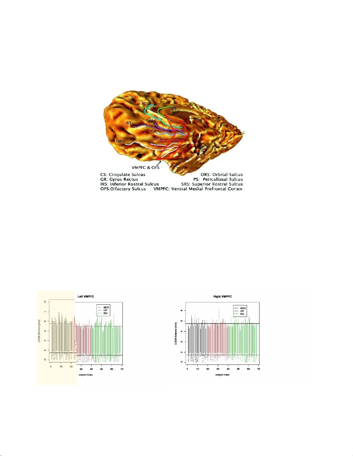
T ec hnical Rep ort # KU -EC-08-2: The Use of Lab eled Cort ical Distance Maps for Quan ti zation and Analysis o f Anatomical Mor ph ometry of Brain Tissues E. Ceyhan 1 , 2 ∗ , M. Hosak ere 2 , T. Nishino 3 , 4 , J. Alexopo ulos 3 , R.D. T o dd 5 , K.N. Botteron 3 , 4 , M.I. Miller 2 , 6 , 7 , J.T. Ratnanather 2 , 6 , 7 Octob er 27, 2018 1 Dept. of Mathematics, Ko¸ c University, 344 50, Sarıyer, Istanbul, T urkey. 2 Center for Imaging Scienc e, Th e Johns Hopkins University, Baltimor e, MD 21218. 3 Dept. of Psychiatry, Washington University Scho ol of Me di cine, St. L ou is, MO 6311 0. 4 Dept. of R adiolo gy, Washington University Scho ol of Me dici ne, St . L ouis, MO 63110. 5 Dept. of Genetics, Washington University Scho ol of Me dici ne, St . L ouis, MO 63110. 6 Institute for Computational Me dici ne, The Johns Hopkins University, Baltimor e, MD 21218 . 7 Dept. of Biome dic al Engine ering, The Johns Hopki ns University, Baltimor e, MD 21218. * corresp onding author: Elv an Ceyhan, Dept. of Mathematics, Ko¸ c Univ ersity , Rumelifeneri Y olu, 3 4450 Sarıyer, Istanbul, T urkey e-mail: elceyhan@ku.edu.tr phone: +90 (2 1 2) 338- 1845 fax: +90 (2 1 2) 338- 1559 short title: Using La beled Cortical Distance Maps for Morphometric Qua ntization k eywords: c o mputational anatomy , depr ession, lab eled cor tica l distance map (LCDM), morphometry , p oole d distances 1 Abstract Anatomical shap e diﬀerences in cortical structu res in the brain can b e associated with v arious neuropsychi- atric and neuro-developmen tal diseases or disorders. Lab eled Cortical Distance Map (LCDM), a recen tly devised tool, can b e a p o werful tool to q u an tize suc h morphometric diﬀerences. In this article, we inve sti- gate v arious issues regarding the analysis of LCDM d istances in relation to morphometry . T he length of the LCDM distance vector provides the num b er of voxels (app ro ximately a multiple of volume (in mm 3 )); median, mo de, range, and v ariance of LCDM distances are all suggestiv e of size, thickness, an d shap e diﬀerences. V arious statistical tests are emplo yed to detect left-righ t morph ometri c asymmetry , group dif- ferences, and stochastic ordering (i.e., cdf diﬀerences) of th es e quantities. How ever these measures provide a crude summary based on LCDM distances which may conv ey much more information about the tissue in question. T o utilize more of this in f ormation, w e p ool (merge) the LCDM distances from sub jects in the same group or condition. W e chec k for the similarity of the distributions of LCDM distances for sub jects in the same group u s ing the kernel d ensit y plots, and also inv estigate the inﬂu ence of the outliers (i.e., sub jects with extremely diﬀerent LCDM distance distributions). The statistical meth odology we employ require normality and within and betw een sample indep endence. W e demonstrate that the v io lation of these assumptions have mild inﬂ uence on th e tests. W e specify the types of alternativ es the parametric and nonparametric t ests are more sensitive for. W e also show th at the p ooled LCDM distances p ro vide p o wer ful results for group diﬀerences in distribution, left-right morph ometric asymmetry of the tissues, and v ariation of LCDM distances. As an illustrative example, we use gray matter (GM) tissue of ventral medial prefrontal cortices (VMPFCs) from sub jects with ma jor depressive disorder, sub jects at high risk, and con t ro l sub jects. W e ﬁ n d signiﬁcant ev idence that VMPFCs of sub jects with depressive disorders are diﬀerent in shap e compared to th o se of normal sub jects. Although the metho d ol ogy used here is applied on the LCDM distances of GM of V MP F C, it is also v alid for morphometric measures of other organs or tissues and distances similar t o LCDM distances. 2 1 In tro duction Quantiﬁcation of morphometric pro perties of neo cortical tissues is a ma jor comp onen t of Computational Anatomy [1-21]. Our g roup recently developed the La beled Co r tical Distance Ma pping (LCDM) techniques [22] whic h was shown to b e useful in identifying cortical thinning in the cingulate co rtex in sub jects with Alzheimer’s Disease [23] and in sub jects with s c hizophrenia [24] in compar ison to c on trol sub jects. Cortical thinning has b een o bserv ed in other reg ions in a v ariety of neuro-developmental and ne ur o- degenerative disorder s (see ab ove references for examples ). In par ticular, functiona l imaging studies implicate the ven tra l medial prefrontal cor tex (VMPFC) in ma jor depress ive disorder s (MDD) [25, 26] which hav e bee n correla ted with sha pe changes observed in structura l imaging s tudies [2 7, 28]. The pr efron tal cortex , tog ether with amygdala and hipp ocampus, plays a n imp ortan t r ole in mo dulating emotions and mo od. Structural imaging s tudies in MDD have larg e ly fo cused on adult onset with only few fo cused on e arly onset MDD which has b een asso ciated with structural deﬁc its in the subgenual prefrontal cortex , a subregion of the VMPFC [28]. F urthermore, the whole VMPFC has bee n examined in a twin study of ear ly o nset MDD [29]. Several studies of the VMPFC and related s tr uctures hav e b een o btained fro m ana ly sis of the cor tex as a whole [4 ,17, 30, 3 1] whereas o thers have pursued a mor e lo calized analys is attempts to dea l with the highly folded gr a y/ w hite matter cortex [32]. In this way the laminar sha pe o f the brain tissue ca n b e quantiﬁed in great detail. Two asp ects o f the laminar sha pe are structural formation (like s ur face and form of the tissue) and s cale or size (like volume and surface area ). Thro ughout the article, we call all asp ects of laminar s hape as the morphometry of the tissue (including s hape and size), the surface s tructure a nd for m will be referr ed as “shap e” and scale will b e r eferred as “size ” . The ﬁrst step in creating LCDM metrics inv olves segmenting MRI subvolumes of the tissue in question. Then every vo xel is lab eled by tissue type as gray matter (GM), white matter (WM), and cerebros pina l ﬂuid (CSF). F or every vo xel in the imag e volume, its (norma l) distance from the center o f the vo xel to the close s t po in t on GM/WM surface is co mputed. A signed distance is used to indicate the lo cation of ea c h voxel with resp ect to the GM/WM s urface; distances are p ositive for GM and CSF voxels, and nega tiv e for WM vo xels. See Figure 1 for a schematic ﬂowc hart o f the LCDM pro cedure a nd Figure 2 for a tw o-dimensio nal illustration of LCDM distance ca lculation and non-nor malized histogra ms o f the (signed) dista nces for GM, WM, a nd CSF. As an illustrative example, we in vestigate GM tissue in VMPFCs in a study of early onset depress ion in twins. Previous ly , we a nalyzed v ar ious morphometric measur es (i.e., volume, des criptiv e statistics bas ed on LCDM distances such as median, mo de, rang e, and v ariance) a nd demonstrated that e x cept for left-right asymmetry and cor r elation b et ween left and rig ht measures, these v aria bles usually faile d to discriminate the healthy sub jects from depressed ones [3 3 ]. One reas o n for this is the fact that the sub jects in o ur data set are age-matched female twins, who p otent ially hav e VMPFCs similar in size. Moreov er, this might be partly due to the size of gro ups; i.e., if w e ha d more participants in the s tud y , these measures would hav e bee n mor e likely to yield signiﬁcant diﬀerences b et ween the gr o ups. On the other hand, by o nly using a descriptive summary statistic of numerous of dis tances for each per son, we es sen tially lose most of the information provided b y LCDM measures. In this article we provide a s trategy to avoid this information lo s s by p o oling the LCDM distances. W e us e the po oled (by condition or group) distances to detect morphometric diﬀerences such as diﬀer e nces in shap e, size, thickness v ariation, and left-rig ht asymmetry . How ever there is a downside to p ooling, the po oled distances do no t have within sa mple indep endence, as the distances of neighboring voxels for ea c h voxel at a particular hemis pher e o f a p e rson are dep enden t. Moreov er, ther e is also dep endence b et ween distances from left and r igh t VMPFCs of ea c h sub ject. W e demonstra te that within sample dep endence do es no t aﬀect the tests in ter ms of empirical signiﬁcance levels (or Type I erro rs) o r power; and left-right dep endence o nly makes the asy mm etry tests less powerful than they could hav e b een. W e descr ibe the acquisition of LCDM distances for VMPFCs in Section 2 .1, the metho ds we employ in Sections 2.2 , descr ibe the example data set in Section 2.3, provide analysis of volumes and des criptiv e measures based on LCDMs in Section 3, outlier detection in Section 4 .1 , analyz e the p oo led dis ta nces in Section 4 .2, and present the inﬂuence of as sumption of violatio ns in Sec tio n 5. In [33] we computed simple descriptive measures for each left a nd right VMPFCs o f the sub jects a nd analyze d these measures for gro up diﬀerences. These LCDM-based de s criptiv e s ta tistics ar e also a nalyzed in more detail in this article. F or more technical detail on LCDM see, e.g., [36], where accur acy of LCDMs and v ar iabilit y of cortica l mantle distance proﬁle s 3 are also discussed. In [36], LCDM is used for detecting diﬀerences in cingulate due to dementia of Alzheimer’s t yp e (DA T). The usual W elch’s t -test is applied for volume compa r isons, Wilcoxon r ank sum test is applied for group co mparisons on randomly s elected subsamples fro m LCDM distances. In this article, ra ther than subsampling or summarizing , we use the entire LCDM distance se t by p ooling the distanc e s for ea c h group and inv estigate the v alidity of the under lying ass umptions for the tes ts used. Since in this article we fo cus on the use of LCDM distance s , r a ther than the clinical implications o f the genetic inﬂuence (due to twinness), we ignore the twin inﬂuence for most o f the curr en t analysis. 2 Metho ds 2.1 Data Acquisition A cohor t of 34 r igh t-handed young female twin pairs b et ween the a g es o f 1 5 a nd 24 years old were obtained from the Missour i Twin Registry and used to study cortical changes in the VMPFC asso ciated with MDD. Both monozygo tic and dizygo tic t win pa irs were included, of which 14 pa ir s were controls (Ctrl) and 20 pairs had o ne twin aﬀected with MDD, their co-twins were designated as the High Risk (HR) gro up. Three high resolution T1-weight ed MPRAGE magnetic res onance scans of this p opulation were acquired using a Siemens sc a nner with 1 mm 3 isotropic resolution. Images were then averaged, c o rrected for intensit y inhomogeneity and interpolated to 0 . 5 × 0 . 5 × 0 . 5 3 isotropic vo xels. F ollowing Ratnanather et a l. [32], a reg io n of in ter est (ROI) comprising the prefro n tal co rtex stripp ed o f the basal g anglia, eyes, sinus, cavit y , and temp oral lob e was de ﬁned ma n ually a nd segmented into gr ay matter (GM), white matter (WM), and cerebro s pinal ﬂuid (CSF) by Bay es ian segmentation using the expe c tation maximization a lgorithm [3 4]. A triangulated r epresen tation of the cortex a t the GM/WM bo unda ry w as generated using isosur face a lgorithms [35]. See Figure 1 for the schematic ﬂowc hart of LCDM measurement pro cedure and Figure 2 for an illustra tion of norma l distances from GM and WM voxels to the interface in a tw o-dimensional setting and non-normalized histograms of LCDM distances fo r GM, WM, a nd CSF tiss ues of a cingulate tissue. The GM tissue comprises most of the cor tex; and by co nstruction, most of GM distances are p ositive, mo st of WM distances are negative, and all of CSF dis tances a r e p ositive. The mismatch of the signs for so me GM and WM vo xels clos e to the GM/WM b oundary ar e due to the wa y the surface is constructed in re la tion to how the pixels are lab eled, such that a sur fa ce is alwa ys intersecting pixels, and has to maintain a somewha t smo oth shap e. So some appropria tely lab eled GM and WM pixels may fall o n a side of surface that they s ho uld not b elong to; how ever, these misla beled voxels constitute a small num b er of vo x els and do not aﬀect our ov er all analysis. Le t V b e the reg ular la ttice of vo xels deﬁning the regio n of interest, S (∆) b e the triangulated graph representing the smo oth b oundary at the GM/WM sur f ace. Then the distance computation algor ithm is sp eciﬁed as [36-38 ]. for all v i ∈ V do s closest ← a po in t in S (∆) s uc h that for all s j ∈ S (∆) do d ( s closest , v i ) ≤ d ( s j , v i ) end for D i ← d ( s closest , v i ) end for where d ( · , · ) stands for the usua l Euclidean distance , v i is the i th vo xel, s j is the j th po in t in S (∆) a nd D i is the i th distance (i.e., distance for i th vo xel). That is, an LCDM distance is a set distance function d : v i ∈ V → d (cen troid( v i ) , S (∆)), which is the distance b et ween the centroid (or center of mass) of v i and the set S (∆). More precisely , D i := d (centroid( v i ) , S (∆)) = min s ∈ S (∆) k cen troid( v i ) − s k 2 T o distinguish the dis tances for voxels from diﬀerent tiss ue types, we denote the distance for i th vo xel in tissue type lab el as D i ( la bel ) for l abel ∈ { WM,GM,CSF } . 4 V olume and GM distr ibut ions as a function of p osition from the GM/WM interface can b e derived fro m LCDMs. The GM volume is simply the tota l num b er of GM voxels (times the v olume of a single v oxel). As v ariability of to tal GM volume ca n be a confounding factor in studying cortical thickness, nor malizing LCDMs of each individual by its total GM volume gener ates Cor tical Mantle Distance (CMD) proﬁles. Integrating the density function r esults in a distribution function that repres e n ts the p ercen tage of GM as a function of distance from the cor tica l sur f ace. 2.2 Statistical T ests W e use v ar ious morphometric measures of left (and r ig h t) VMPF Cs in our analysis. LCDM dista nc e measures are suﬃcient to determine the volumes (in mm 3 ) of VMPFCs. F or each p erson, we als o rec ord the median, mo de, range, and v aria nce of LCDM distances. F or left (and right) volume, media n, mo de, ra ng e, and v ariance compariso ns b et ween gro ups , w e ca n not apply K rusk a l-W allis (K-W) test for equality of the distr ibut ions of thes e meas ures for all groups, b ecause there is an inherent (genetic) dep endence b et ween MDD and HR groups, since co t win o f each MDD sub ject is by deﬁnition a HR sub ject. So we use Wilcoxon rank sum test to compar e MDD and Ctr l VMPFC, and als o HR and Ctrl VMPFC. On the other ha nd, we use Wilcoxon signed rank test for MDD and HR VMP F C, due to dep endence of the sa mples. Then we a dj ust these p -v a lue s for simultaneous pair wise comparis ons by Holm’s co rrection metho d. Se e [45] for the tests and [39] for Holm’s correctio n. W e r e s ort to the non-par ametric tests only , when the assumptions o f normality and ho mogeneit y of the v a riances (HOV) are not met. When the a ssumptions are met and only the parametric tests yield signiﬁcant results, w e use the par ametric counter-parts (W elch’s t -test for indep e nden t sa mples a nd paire d t -test). F or morpho metric as ymmetry of left and right VMPFCs, we compare these measures b et ween left and right VMPFCs (ov erall and for each gr o up) by Wilcoxon signed ra nk test which is a paired (for diﬀerences o f measures) test (see, e.g., [40]). W e p erform correla tion analysis b et ween left and rig h t morphometric meas ures using Sp earman’s rank cor - relation co eﬃcien t and the co rrespo nding test aga inst the corr elation co eﬃcient b eing nonzero. W e a lso com- pare cdfs (cumulativ e distribution functions) be tw een gr oups for left (a nd r igh t) VMPFCs using Kolmogo ro v - Smirnov (K-S) test (see, e.g., [40 ]). When we p o ol (i.e., merg e ) the LCDM distances by group, there is a n inher en t dep endence b et ween LCDM distances due to the spatial corr elation b et ween neighbor ing vo xels of a left o r rig ht VMPFC. F or the parametric tests (ANO V A F -test and t -test), the assumptions of normality and within sample independenc e are vio lated, while for nonpa rametric tests (K-W test a nd Wilcoxon tests) only within sample independence is violated. Since more assumptions are viola ted for the parametric tests, the no nparametric tests are exp ected to b e mor e a ppropriate in our ana lysis. Ho wev er, since the co rrelation structure is similar for ea c h p erson (hence for each gro up) , its inﬂuence on bo th parametr ic and nonparametric tests is negligible. See Section 5 for a Monte Car lo simulation study to justify the use of these tests for s uc h data structures. W e use Krusk al- W allis (K-W) test for equality of the distributions of the p ooled distances for all left g roups and ANOV A F -tests (with and without HOV) for equality of the means for a ll left gr oups; if K-W test yie lds a signiﬁcant p -v alue, then we use pairwise Wilcoxon r ank sum test to compare the pair s of the groups; similarly , if one of the ANO V A F -tests is sig niﬁca n t, then we use pairwise t -test to compare the pairs of the groups. Then we adjust these p -v alues for s im ultaneous pairwise compar is ons by Holm’s corre ction method [3 9]. W e per form similar analys is for rig ht g roups. F or morpho metr ic a symmetry of left and right VMPFCs, we compare these measures betw een left a nd right VMPFCs (ov er all and for each gro up) by Wilcoxon r ank s um tes t (see, e.g., [40]) and W elch’s t -tes t. A lthough there is an inherent dependence on the MDD a nd HR VMPF C or left and right distances, we do not use Wilcoxon signed rank test (for dep enden t samples) or matched pair t - test, bec ause the distances for the left and right VMPFCs can no t b e matched (paired). F o r the same r eason, we ca nnot per form corre lation analysis on these g roups. W e also compa re cdfs b et ween gr oups for left (and right) VMPFCs using Ko lmogorov-Smirnov (K-S) test (see, e.g., [40 ]). The tes t of equality or homog eneit y o f the v aria nces (HOV) of p ooled distances is a ls o imp ortan t. Be- cause, v ariance diﬀerences b et ween gro ups might b e indicative of diﬀerences betw een the v ariations o f the morphometry of VMPFCs. Therefor e , we p erform HOV test by using Levene’s test with absolute disp ersion around the median, which is also known a s Brown-F orsythe’s (B- F) HOV test (see, e.g., [41 ]). 5 2.3 Example Data Set As an illustr a tiv e example, we use GM of left and rig h t VMP F Cs. The prefro ntal cortex, together with the amygdala and hippo campus plays an imp ortant r o le in mo dulating emo tions and mo od. F or the lo cation of VMP F C in brain, s ee Fig ur e 3 . Abnormalities have b een demons tr ated in structur e a nd function of the prefrontal cor tex due to depressio n [2 5,26]. Pr evious structura l imaging studies on Ma jor Depressive Disorder (MDD) have larg ely fo cused on adult onset, while o nly few hav e foc us ed on ear ly onset MDD. Botter o n et al. [44] hav e conducted structura l imag ing s tudies on e a rly onset of MDD in the v en tral media l prefr on tal cortex (VMPFC) region o f twins. Structural deﬁcits in the subgenual prefrontal cor tex hav e b een shown to implicate early onset of MDD [29 ]. F or conv enience in no tation, we suppress the la bel argument in the dis tances, as we only co nsider the GM tissue. Let D L be the set of LCDM distances, D L ij k , which is the distance as sociated with k th vo xel in GM o f left VMPFC of sub ject j in gr o up i for j = 1 , . . ., n i and i = 1 , 2 , 3 (group 1 is for MDD, gro up 2 fo r HR, and group 3 for Ctr l). Right VMPFC dista nces D R are denoted similarly as D R ij k . The LCDM distances for GM in left and right VMPFCs, D L and D R , ar e plotted by sub ject in Figure 4. The automated seg men tation is more reliable for the GM close to the GM/WM surface due to the high level o f contrast. How ever, there are still voxels which, althoug h lab eled a ppr opriately , hav e the inco rrect sign, that is, some of D L ij k and D R ij k are negative for ea c h sub ject. Lar ge dis ta nces ar e p o ten tially less reliable, due to the diminishing co ntrast around the bo unda ry of GM and CSF compar tm ent s. Thus, ba s ed on Figure 4 and pr io r anatomical knowledge on VMPFCs (e.g., [42]), we only keep dista nces larger than − 0 . 5 mm so that mislab eled WM is excluded fro m the da ta, and the upp er limit is set to 5 . 5 mm , so that the er ror due to less r eliable large distances is r educed. Observe that in the left VMPFC distances, MDD sub jects 8 a nd 11, HR sub jects 3 and 1 8 , and Ctrl sub jects 6, 10, 11 , 1 2, and 22 s eem to b e more diﬀerent with Ctr l sub jects 11 and 12 being “thinner” while the res t are “thick e r ” than other left VMP F Cs. On the other hand, in the right VMPFC distances , VMPFC of MDD sub ject 4, HR sub ject 5 , and Ctrl sub jects 12 and 2 1 seem to b e mor e diﬀer en t, with VMP F Cs o f HR s ub ject 5 and Ctrl sub ject 12 b eing thinner and the other s being thicker than the rest of the right VMP F Cs. Note that Figure 4 provides a preliminary asses s men t of relia bilit y of LCDM distances, since it do es not provide the distr ibutio na l b ehavior of the distances , but only pr o blems with small (negative) a nd large distanc e s. As a technical a side, we no te that o nly 0 .16 % o f left distances and 0.14 % of right dista nces a re below -0 .5 mm ; on the other hand, only 0.22 % of left distances and 0 .07 % of r igh t distances are ab ov e 5 . 5 mm . 3 Analysis of V olumes and Descriptiv e M ea sures of LCDM Dis- tances of VMPFCs V olume is a mea sure o f size of VMPFCs. Let V L ij be the volume of le ft VMPFC o f sub ject j in gro up i , for j = 1 , . . . , n i and i = 1 , 2 , 3. Right VMPFC volumes are denoted similar ly as V R ij . F o r each p erson, n um b er of L CDM dis tances reco r ded yie ld the num b er o f v oxels, which in turn yie lds a multiple o f the volumes in mm 3 , since each vo xe l is a cub e of size 0 . 5 × 0 . 5 × 0 . 5 mm 3 . Tha t is, V L ij = 0 . 125 × X k I  D L ij k ∈ [ − . 5 , 5 . 5]  where I ( · ) stands for the indicator function. Right VMPFC volumes c an b e obtained similar ly . 3.1 Analysis of V olumes of VMPF Cs W e analyze volumes of VMPFCs for v arious purp oses: (i) to provide an outline of the metho dology we will employ for other qua n tities in this a rticle, (ii) to compare the volume r esults with o ther comparis ons, and (iii) to check the volume (size or scale) diﬀerences due to groups. W e no te the group of e ac h volume v alue; for example, if a volume is of a VMPFC o f a per son in gro up MDD, then the corr esponding gr oup is MDD. See Figure 5 for the (jittered) scatter plot of the volumes by gr oup for left and r igh t VMPFCs. See a lso T a ble 1 for the sample sizes, means, a nd standar d deviations of the v olumes, ov era ll and for each gr o up, for left a nd right VMPFCs. Observe that left VMPFC volumes are larg er than the right VMPFC volumes. Moreov er 6 the mean volume measures fo r the left VMPFC s eem to b e more diﬀerent be tw een gro ups co mpared to right VMPFCs. T o ﬁnd which pairs, if any , manifest sig niﬁca n t diﬀerenc e s, we p erform pa irwise comparis o ns by Wilcoxon rank sum tes ts fo r MDD,Ctrl and HR,Ctrl pairs a nd Wilcoxon signed ra nk test for MDD,HR pair for left VMPFC volumes using Holm’s corr ection. The p -v alues for the pairwise tests for left a nd right VMPFC volumes are pr esen ted in T able 2, where p W stands fo r p -v alue for Wilcoxon r ank sum test, p t stands for p -v alue for W elch’s t -test, signiﬁcant results are ma rk ed with an asterisk (*) and ( ℓ ) stands for the alternative that ﬁr s t g roup volumes tend to be le s s than second gro up volumes a nd ( g ) stands for the alternative that ﬁr st group volumes tend to b e grea ter than second gr oup volumes. More precisely , given t wo groups o f ra ndom v ariables X and Y , ( ℓ ) alternative implies F X ( x ) > F Y ( x ) where F X and F Y are the distribution functions for X and Y , resp ectiv ely , or E [ X ] < E [ Y ] where E [ · ] stands for exp ectation or P ( X > Y ) < P ( X < Y ). Notice tha t all of these v arious forms of alterna tiv es c o n vey the idea that “X tends to be smaller than Y” in some way [40]. O bserv e that none of the pair s manifest signiﬁcant diﬀerences in distribution o f volumes. F or the t - test, ( ℓ ) stands for the alternative that the ﬁrst g roup mean volume is less than the sec o nd group mea n, and ( g ) stands for the alternative that the ﬁr st gr o up mean is g r eater than the s econd gro up mean. None of the pairs indicate signiﬁcant diﬀerences in mean volumes. Since MDD,HR v olumes a re dep enden t, we only test for the homogene ity or equality of the v ariances of volumes of MDD,Ctrl a nd HR,Ctrl pair s . W e o bserv e that HOV of MDD a nd Ctrl left VMPFC volumes is not re j ected ( p = . 3 610), and likewise fo r HR and Ctr l le f t VMPFC volumes ( p = . 3202 ). Similarly , HOV of MDD and Ctrl rig h t VMPFC volumes is not rejected ( p = . 10 38), a nd likewise for HR and Ctrl right VMPFC volumes ( p = . 1038). This suggests that the sprea d o r v ariation in volumes of left (and r igh t) VMPFC within groups is not signiﬁcantly diﬀerent fro m each other for the gro ups co ns idered. W e also test fo r the diﬀerences b et ween left a nd right VMPFC volumes, i.e., left-rig h t volumetric asym- metry . F or the asso ciated p -v alues, see T able 3, where p W stands for the p -v alue for Wilcoxon s igned r ank test, and p t stands for pair e d t - tes t. F or testing ov erall left-right asymmetry , we po ol all the left volumes into one set, and all the r igh t volumes into ano ther. Observe that left VMPFC volumes a re signiﬁcantly larger than right VMPFC volumes ( p W = . 00 64 and p t = . 0087 ). Among the groups, only MDD VMPFC shows signiﬁcant volumetric left-rig h t asymmetry with p W = . 0360 and p t = . 0233 . Tha t is, the depressed sub jects tend to hav e more left-right volumetric asymmetry c ompared to HR and Ctrl sub jects, in such a way that left volumes tend to b e s igniﬁcan tly larger than the right volumes in MDD s ub jects. Spea rman’s rank corr elation c o eﬃcients, denoted ρ S , a nd the asso ciated p -v alues betw een the left and right scales a re given in T able 4, where MDDL r efers to volumes of left VMPFC of MDD patients, MDDR, HRL, and HRR are deﬁned similar ly . Observe that there is signiﬁcant (po sitiv e) corr elation between the left and rig h t v olumes for overall, MDD, HR, and Ctr l VMP FCs. Correla tio n implies that, for example, when left volumes increas e or decr ease, so do the rig ht volumes. On the other hand, MDD,HR left volumes are mildly correla ted, while MDD,HR r igh t volumes are not signiﬁca n tly cor related. W e also co mpare the cumulativ e dis tribution function of the volumes by group, which may also provide a sto c ha stic ordering , for MDD,Ctrl and HR,Ctrl pairs only , since the MDD,HR pair s are dep enden t. See T able 5 for the a ssociated p -v alues. O bserv e that none of the p -v alues is signiﬁca n t. Notice that e x cept for left-right asymmetry and corr elation b et ween left and right v o lumes (for each gro up) , none of the compa r isons is signiﬁcant at .05 level. But this do es not necessa rily imply la c k o f VMPFC shap e diﬀerences b et ween gro ups, as volume only measures a n asp ect of size. Next, we analyze v ar io us descr iptiv e measures (summary statistics ) based on GM LCDM distances. The lack of sig niﬁcan t group diﬀerences in volumes might b e due to the fact that the data co nsists of age-matched female sub jects, who se VMPFCs might b e very similar in size. F ur ther more, if the num b er of sub jects p er group is incr eased, then it is more likely to see signiﬁcant gr oup diﬀer e nc e s, if they exist. 3.2 Analysis of Descriptiv e Measures of LCDM Distances of GM of VMPF Cs In this section we a nalyze some other measures which are mor e directly asso ciated with LCDM dista nces. W e ﬁnd the descriptive measure s (summary statistics) o f the LCDM dista nces for ea ch per son. Among the descriptive statistics we analyze ar e the median, mo de, ra ng e, and v aria nce of the LCDM distances. W e 7 conduct the tests that we used for volumes in Se c tion 3.1 on these descriptive meas ures. Note that each of these desc r iptiv e mea sures conv eys infor mation a bout some asp ect o f morphometry (shap e and s ize) of VMPFCs. W e provide these analys is to demonstra te how LCDM distances can b e used as a simple compara tiv e to ol. The m edian of LCDM distances for VMPFCs yields a ce ntral distance measure, or distance fr om “center” of VMPFC GM to the GM/WM in terface. The median distance for left and right VMPFC gray matter for sub ject j in gr oup i are deno ted as med  D L ij  and m e d  D R ij  , resp ectiv ely . W e use the median dis tance rather than the mean distance here, b ecause LCDM distances are skew ed r igh t, so median is a b etter measure of centralit y as it is mor e r obust to extreme v alues compar ed to the mean. Se e Figure 4 for right skewness of distances in the scatterplo t and Figure 6 for the kernel density plo ts for LCDM distances for left and r igh t VMPFC by sub ject. The tests indicate that there is no g roup diﬀere nc e s in the dis tributions of the median distances for b oth left and right VMP FCs, no sig niﬁca n t left-right as ymmetry , a nd no signiﬁca nt diﬀerence betw een the cdfs of median distances of gr oups for b oth left and r igh t VMPFCs. HOV is rejected for HR and Ctrl left media n distances with p = . 0261 only . F urthermore, MDD,HR, and Ctrl-left,Ctrl-rig h t median distances are signiﬁcantly p ositiv ely co rrelated, while MDD,HR left (a nd right) median distances are not. The m ode of a data set as a descr iptiv e statistic is the most frequent observ a tion in the data set. T o make it more meaningful for our data, we rounded the distances to 1 decimal place. Hence mo de corresp onds to the ten th of a millimeter that co n tains the most num b er of GM vo x el distances . F or instance, if mo de of a sub ject is 2 .2 mm the mos t num b er o f distances a re in the interv al [2 . 2 mm, 2 . 3 mm ] compared to other interv als. More precisely , the mo de of LCDM distances for VMPF C y ields the distance fro m the “widest” strip para llel to the GM-WM interface. The mo de of distances fo r left a nd right VMP F C gray matter for sub ject j in group i are deno ted as mode  D L ij  and mode  D R ij  , resp ectiv e ly . The tests indica te that ther e is no g roup diﬀerences in mo de of the dista nces for b oth left and rig h t VMP F C, no signiﬁcant left-right a symmetry , no signiﬁcant v a riance diﬀerence of mo de of distances b et ween gro ups, a nd no sig niﬁca n t diﬀerence b e t ween the cdfs of the mo des of the distances b et ween groups for b oth left and r igh t VMPFCs. There is mild p ositiv e correla tion b et ween Ctr l-left,Ctrl-righ t mo des, a nd MDD,HR rig ht mo des. The range of LCDM distanc e s for VMPFCs yields a roug h measure of “ th ickness” of GM of VMPF C. W e use the range (maximum LCDM distance min us minimum L CD M dista nce) rather than the ma xim um distance here, although co nceiv a bly the la tter is also a reaso nable choice. The range of dista nces for left a nd right VMPFC g ra y matter for sub ject j in gro up i ar e denoted as rang e  D L ij  and r ang e  D R ij  , r espectively . The tests indicate that ther e is no gro up diﬀerences in range of distances (thic k ness) for b oth left a nd r igh t VMPFCs, no signiﬁcant diﬀerences b et ween the cdfs o f groups for b oth left and rig h t VMPFCs, and HOV of r anges of g r oups is not r ejected. Left distance ranges are sig niﬁcan tly larger than right distance ra nges, ov era ll and for each gr oup. F urthermor e, there is mild p ositiv e correla tion b et ween Ctrl-left,Ctrl-right ranges, and MDD,HR right ranges . The v ariance o f LCDM distance s for VMPF C yie lds a measure of “v ar ia tion” of size o f GM in VMP F C. W e use the v aria nces, r ather than s tandard deviatio ns here, since b oth yield the same res ults under rank ba sed non-para metr ic tests. The v aria nce of distances for left and right VMPFC g ra y matter for sub ject j in gr oup i a re deno ted as V ar  D L ij  and V ar  D R ij  , res pectively . The tests indicate that there is no group diﬀerence in v ariance of dista nces (size v a r iation) for b oth left and right VMPFC, and no sig niﬁcan t diﬀerence b et ween the cdfs of v ariances of dis tances b et ween gr oups for b oth left and right VMP FCs, and HOV of v aria nc e s of groups is no t rejected. The r e is signiﬁcant left-right as y mmet ry in v a r iance o f distances, with left v aria nces signiﬁcantly larger than right v ariances , ov era ll and for each group. F ur th ermore, there is mild corr elation betw een MDD left and right v aria nces. Although descriptive statistics of LCDM distance s measure so me mor phometric asp ect of VMPFCs, they usually fail to discriminate the healthy VMPF Cs from depress ed VMPFCs. One rea son for this is the fac t that the sub jects in our data set ar e ag e-matc hed female twins, who p oten tially hav e similar size VMPFCs. Moreov er, this might b e par tly due to the siz e of gro ups; i.e., if we had more participants in the s tudy , these measures ar e more likely to yield signiﬁcant diﬀere nce s b et w een the gr oups. O n the o ther hand, by only using a descriptive summary statistic of thousands of distances for ea c h p erson, we e ssen tially lo s e mos t of the information LCDM mea sures conv ey . T o avoid this ov er-summariza tion, we will use all the distances in our analysis in the next section. One could a ls o use other descr iptiv e measur es such a s inter-quartile rang e (IQR), skewness, and kurtosis 8 of the LCDM distances. 4 P o oling LCDM Distances Since the descriptive measur es of LCDM distances ar e summary statistics, they tend to ov ers implif y the data[33], a nd hence we los e most of the information convey ed by the LCDM distances . T o av o id this informa- tion loss, we p ool LCDM distances of s ub jects from the same gr o up or condition; that is, we p ool the LCDM distances of a ll left MDD VMPFCs in o ne gr oup, those of a ll left HR VMPFCs in one gr oup, and those of all left Ctrl VMPFCs in one gro up. That is, D L iℓ = n i [ j =1 D L ij k where D L iℓ is the ℓ th distance v alue for distances from sub jects in group i . W e p oo l the right VMPFC LCDM distances in a similar fashion and denote the rig h t po oled distances as D R iℓ . One of the underlying assumptions is that the distances from VMPFC of sub jects with MDD have the same distribution, thos e of HR hav e the sa me distr ibution, and so do those of Ctrl gr o up. In other words, we assume that D L ij k are identically distributed for all j = 1,. . . , n i and i = 1 , 2 , 3 . So, D L ij k ∼ F L i for all j, k , and likewise D R ij k ∼ F R i for a ll j, k . Hence the po oled distances are distributed as D L iℓ ∼ F L i and D R iℓ ∼ F R i for i = 1 , 2 , 3 . W e take this action under the presumption that the morphometry o f VMPFCs ar e a ﬀ ected by the condition in a simila r wa y and hence ag e and g ender matched sub jects with the same condition should hav e VMP F Cs similar in morphometry . As a prec a utionary step, we ﬁnd the extr eme (outlier) sub jects; i.e., the sub jects whos e VMPFCs have muc h diﬀere n t distributions than the rest in Section 4.1 by (sub jectively) comparing the kernel density estimates. 4.1 Outlier Detection b y Using Kernel Densit y Plots When p o oling the distances for s ub jects at a particula r gro up, we implicitly assume that the distance s for s ub jects in the same group hav e identical distributions. As a precautionar y step, we ﬁnd the extr eme ( outlier ) sub jects; i.e., the sub jects with VMPFCs having muc h diﬀerent distributions than the r est. In Figure 4, obs e rv e that in the left VMPFC distances , MDD sub jects 8 a nd 11, HR sub jects 3 and 18 , and Ctrl sub jects 6 , 10, 1 1, 12, and 22 seem to b e more diﬀerent with Ctrl sub jects 11 and 12 b eing “ thinn er” while the r est ar e “thick er” than other left VMPFCs. O n the other hand, in the rig h t VMPFC dis ta nces, VMPFC of MDD sub ject 4, HR s ub ject 5, and Ctr l sub jects 12 and 21 seem to b e mor e diﬀerent, with VMPFCs of HR sub ject 5 and Ctrl sub ject 12 b eing thinner and the others b eing thick er than the rest o f the right VMPFCs. Note that Fig ure 4 provides only a prelimina r y asses smen t of reliability of LCDM distances, since it do es not provide the distributional behavior of the distance s, but only p oin ts the pro ble ms with sma ll (negative) and large (po sitiv e) distances. Hence the kernel densit y e stimates (or normalize d histograms) ca n serve as a be tter explor atory to ol to detect o utliers. See Figure 6 for the kernel density estimates of LCDM distances plotted by sub ject. Notice that these kernel density es tima tes are nor malized for volume, a s each density curve has the sa me unit a rea under it. Reca ll also that Figur e 4 pr ovides some insight on kurtosis (the thickness of le f t and r ig h t tails ) of the distr ibut ions of LCDM dista nces. Using b oth Figur es 4 and 6, we observe that LCDM distances for s o me sub jects hav e very diﬀerent distributions tha n the o thers; i.e ., they are outliers. How ever, although Figure 4 provides informa tio n ab out the tails (i.e., sma ll or la rge distances), Figure 6 is more reliable to detect the outliers as it is nor malized fo r volume and pr ovides infor mation for all distance v alues. The VMPFC of o utlier s ub jects are extr e mely diﬀere nt in shap e from the rema ining sub jects in each gro up. Hence an outlier VMPF C in a gr oup do es no t repre sen t an av e rage VMP FC in that group and this discrepancy (extremeness) might be due to so me o ther factor aﬀecting that sub ject only . A careful inv es tigation shows that, among the left VMPFCs, MDD sub jects 1 and 9 , HR s ub jects 3 a nd 1 2, and Ctrl sub jects 6, 10 , 11, 12, and 19 ar e outlier s, while among the rig h t VMPFCs, MDD sub jects 7 , 11, 13, 15, 18, 19, and 2 0, HR sub jects 4, 8, 14, and Ctr l sub jects 4, 1 0, 11, 1 2, 25, and 26 seem to be the outliers. Ther efore, we remov e these sub jects in our p ooled distance data sets, but p erform ana lysis on bo th the po oled distances with a ll sub jects included and the po oled distances without the o utliers a nd remark on how the outliers inﬂuence the co mparisons. Notice that HR le ft sub ject 3, Ctrl left sub jects 6, 10, 11, 12, 9 and Ctrl right sub ject 1 2 a re the sub jects deemed as outliers by b o th of Figures 4 a nd 6. Observe a lso that LCDM dista nce s (mor e pr ecisely the normaliz e d histog rams or kernel density estima tes ) can b e used as a n explorato r y to ol to detect the outliers. Here it may seem a little excessive to use the term “outlier” as the num b er of sub jects that ar e deﬁned as outliers seem to b e numerous. Approximately 15% of left-VMPFCs ar e deﬁned as o utliers, while over 20% of right-VMPF Cs are c la ssiﬁed as outliers. This might see m to o high to trea t these sub jects as outliers, there by suggesting that some form o f mixed distribution mo deling may b e mo re appropr ia te. Although keeping the outliers changes the results co nsiderably compared to results from deleting the o utliers, for the metho ds based on po oling the distances, w e r ecommend removing the outliers, p erhaps in a more conser v ative manner than ours, b ecause the basic premise of p oo ling is bas ed on the similar it y of the distance distributions for VMPFCs of the same group. The issue of mo deling the distances with mixed distr ibutions is a to pic of o ngoing res earc h. See Figure 7 for the kernel densit y estimates of p oo led LCDM distances when the outliers are r emo ved. See also T able 6 for the corres p onding sa mple sizes, means, and standa rd deviations of the p o oled LCDM distances, overall and for e a c h gro up. Obser v e tha t the dens it y proﬁles of LCDM distances for the left VMPFC of MDD and HR s ub jects seem to be very similar while bo th a re diﬀerent fr o m that of C tr l sub jects. On the other hand, there seems to b e more separ a tion be tw een the density proﬁles in r igh t VMPFCs. After removing the extreme sub jects, the s ample sizes of LCDM dista nces hav e decreased while the medians and standard devia tions (hence the v ariance s ) for a ll left and rig h t gro ups hav e increas ed. F urthermore, mean LCDM distances for left VMPFC g ot sma ller, while for right VMPFC the mean distances hav e incr e a sed. F urthermor e, the order of mean distances for left a nd right VMPF Cs do not change with all the sub jects included and when outliers remov ed. F or left VMPFCs, the o rder of mean and standard deviations are HR < MDD < Ctrl (more accur ate notation would b e me an  D L 2  < me an  D L 1  < me an  D L 3  , which w e shor ten for conv enienc e ), while the order of medians is MDD < HR < Ctrl. The change in the order of means a nd medians is due to the levels of rig h t skewness of the distributions. F or right VMP FCs, the o rder o f means, medians, and standard deviations are HR < MDD < Ctrl. Thus, we obser v e that the outliers in the right VMPFC, although inﬂuence the means, medians, a nd v aria nces, do not change their order. 4.2 Results 4.2.1 The Equali t y of the Distributions of Pool ed LCDM Distances First we address the diﬀerences in the distributions in lo cation but not in s pread. The diﬀer e nc e s in the distributions in the lo cation (e.g., means or medians) of LCDM distances imply shap e diﬀer e nc e s. Hence, we test the equality of the distributions o f the left (p ooled) distance s b et ween g roups; i.e., H o : F L 1 = F L 2 = F L 3 where F L i is the distribution function of the p ooled distances fo r group i = 1 , 2 , 3. Likewise for rig h t p ooled distances. The left and rig h t p ooled distances fo r each group are signiﬁca n tly non-no rmal with p L < . 0001 for each test where p L is the p -v alue for Lilliefor ’s test of normality (see, e .g., [43]), p ossibly due to heavy right skewness of the de ns ities. Moreov er, HOV is rejected with p B F < . 0001 for bo th left and rig h t p oole d distances where p B F is the p -v alue fo r B-F test. Hence non-pa rametric tests o f group compariso ns ar e more appropriate for this data. Note that the ab o ve hypothesis o f equality of the distributions of the p ooled distances ca n b e attributable to the similar ity in the VMPFC shap es for all groups, but not vice versa (i.e., the equality of the distr ibutio ns do es not necessar ily imply morpho metric s imila rit y , but s imilarit y in the distance structure of GM tissue with r e spect to the GM/WM s urface.) Notice that LCDM distances ana lyzed in this fashion provide morphometr ic infor mation, on cortica l mantle thic kness and shap e, but the width (the length of VMPFC parallel to the GM/WM sur face) is less relev ant. Because the compar ison is done o n the ra nking of distances with resp ect to the GM/WM surfa c e. F or example, suppo se t wo VMPFC tiss ue s are comp osed of 100 and 10 00 voxels of similar distances and then the test will detect no diﬀerence, altho ugh the mor phometry is o b viously diﬀerent. Hence, a s long a s the vo x e ls are at a similar distance fro m the GM/WM surface, their abundance will not b e inﬂuencing the test r esults. The equality of the distributions of the dis tances of left VMPF Cs is rejected with p K W < . 00 01 where 10 p K W is the p - v alue for K-W tes t, and likewise for rig h t VMPFC distance s ( p K W < . 0001). Without removing the extreme s ub jects (i.e., when all sub jects a re included), we hav e the same conclusions for right and le ft VMPFCs with p K W < . 0001 for bo th. Hence, we p erform pairwise compa risons by Wilcoxon rank sum tes t for left (and right) VMPFC dis tances, using Holm’s corre ction for multiple compariso ns. The p -v a lues adjusted by Holm’s c o rrection method for the simultaneous pair w is e comparis ons for left and right VMPFC distances are presented in T able 7. Observe that, with all sub jects included and when the outliers are removed, MDD- left and HR-le ft distances are not s igniﬁcan tly diﬀerent ( p W = . 3022 for former, p W = . 0776 for latter where p W is the p -v alue for Wilcoxon rank sum test), while b oth tend to be signiﬁcantly less than Ctr l-left dista nces ( p W < . 0 001 for all). Hence, the VMPFC left distances tend to decrea se due to the depressive disorder s, po ssibly due to a thinning in left VMPFCs. In r igh t VMPFC distances, with all the sub jects included, we observe that MDD and HR-right distances a r e not sig niﬁcan tly diﬀerent from each other, while b oth tend to b e signiﬁcantly smaller than Ctrl-right distances ( p W < . 0001 for b oth). When outliers ar e removed, we observe that MDD-right distances tend to b e sig niﬁcan tly sma ller than HR-right distance s ( p W = . 0084 ) which tend to b e signiﬁcantly smaller than Ctrl-right distances ( p W < . 00 01 for b oth). Obse r v e that outlier s (althoug h do not change the order of mean p oo led distances) do inﬂuence the results, in particular for MDD a nd HR groups. Looking at the k ernel density estimates in Figur e 6, w e see that the outlier s in the HR g roup ar e more simila r to MDD g roup, hence making the MDD a nd HR distance dis tributions mor e simila r than ch ance. Recall that we were not able to detect these diﬀerences by using volume, or simple descriptive mea s ures based on LCDM [33 ]. Thus, the p o oled LCDM distances provide co mparisons that are mor e powerful to detect group diﬀerences. Since the densities o f the distances ar e skew ed r igh t, these diﬀerences do not reﬂect the o r der in the mea n distances, but rather the o rder in the median dis tances. F ur thermore, in these analysis w e ig no re the inﬂuence of p ossible dep endence betw een twin pairs due to genetic similar it y . 4.2.2 Homogenei t y o f the V ariances (HOV) of Pool ed LCDM Distances Observe that K-W and Wilcoxon tes ts suggest sha pe diﬀerence s when rejected, in particular the direction of the alterna tives might indicate cor tical thinning. Similarity of the mo rphometry of VMP F Cs will ca use similarity of LCDM dista nc e s, which in turn implies simila rit y of the v ar iances of LCDM distances. V aria nce of distances is s uggestiv e of morpho metric v aria tio n in VMPFCs. So similar shap es and sizes imply s imilar v ariances, but not vice versa. F or example, cor tical thinning will r educe the v ariation in LCDM distance s; and the larg er the spread in the b oundary (surfa c e ) o f VMPFC, the large r the v aria nce of LCDM dista nces. Hence, we test the equality of the v aria nces of the left (po oled) distances b et ween groups; i.e., H o : V ar  D L 1 ℓ  = V ar  D L 2 ℓ  = V ar  D L 3 ℓ  where D L il is the v ariance of the p o oled distances for group i = 1 , 2 , 3. Likewise for right dista nces. With all the sub jects included a nd when extreme sub jects are r emo ved, HOV is rejected with p B F < . 0001 for b oth left and r igh t VMPFC. See T able 8 for the corresp onding p -v alues for s imultaneous pair wise comparis ons adjusted by Holm’s cor rection metho d. With all the sub jects included a nd when the extreme s ub jects are remov e d, the order of the v ariances is HR < MDD < Ctrl for b oth left a nd right VMPFCs with p B F < . 0001 for all six po ssible compa risons. This implies that the morphometr ic v ariation reduces in left and right VMPFCs due to suﬀering from or being at hig h r isk for depressive diso rders compa red to Ctrl sub jects and is smallest for the HR sub jects for bo th left and r igh t VMPFCs. Obser ve that b oth Wilcoxon ra nk sum tests (for lo cation) and B-F tests (for v ariances) yield s igniﬁcan t res ults with the same order ing betw een gro ups (HR < MDD < Ctrl), which might b e due to co rtical thinning among other factors . 4.2.3 Morphometric Left-R igh t Asymm etry wi th P o oled Dis ta nces LCDM dista nces can als o b e used to detect left-rig h t mor phometric asymmetry , which mig h t b e due to s hape or size as ymmetry betw ee n left and r igh t VMP FCs. If the left a nd right VMPFCs a re similar, then the distributions of the left and rig h t VMPFCs will b e similar, but not v ice versa. But, if the distributions of the left and right VMPFCs are diﬀerent, then there is evidence for morphometric left-right asymmetry , which can also b e detected by the use of LCDM distance s (with Wilcoxon rank sum test). In terms of size a symmetry , LCDM emphasizes mantle thickness asymmetr y , ra ther than the mantle width asy mm etry . 11 Hence we test H o : F L i = F R i for each i = 1 , 2 , 3. See T able 9 for the as sociated p -v alues, which are adjusted by Ho lm’s correctio n metho d. Observe tha t when a ll the sub jects ar e included, le ft dis ta nces a re signiﬁcantly larger than r ig h t distance s, ov era ll, and by g roup with p W < . 0001 for each test. When extr eme sub jects (outlier s) ar e remov e d, Ctrl and MDD VMPFC distances yield signiﬁca n t left-right a symmetry , with left distances b eing sig niﬁcan tly smaller than rig ht distances ( p W < . 000 1 for b oth); a nd HR-left dista nces are signiﬁca n tly la rger than HR- right distanc e s ( p W = . 001 5). Hence, we co nclude that there is signiﬁcant left-right a symmetry in LCDM distances. How ever, the direction of left-right a symmetry is diﬀerent for MDD a nd HR sub jects, while it is same for MDD and Ctrl sub jects. This sugges ts that cor tical mantle in left VMPFC is thinner for MDD and Ctrl sub jects and thick er for HR sub jects co mpared to their right counterparts. Notice tha t the inclus io n of outliers (i.e., when all sub jects are included) inﬂuences MDD and Ctrl gr oups to the extent that the direc tio n of the asymmetry is reversed. 4.2.4 Sto c hastic O rdering of Pool ed LCDM Dis ta n c es Recall that we used Wilcoxon tests to test the null hypothesis of equality of the distributions , i.e., H o : F X = F Y where F X and F Y are the distributions of v ariables X and Y , re s pectively . F or one-sided alter na tiv es, the p -v alues based on Wilcoxon test ar e complementary (i.e., the p -v a lue for “ < ” and “ > ” alter nativ es add up to 1). Hence p - v alue will b e signiﬁcant for only one type of directiona l alternative. F urthermore , when rejected, Wilcoxon test implies an order ing in lo cation par ameter such as mea n or median. Sto c hastic or dering, if present, c an b e deduced fro m the directio n o f the a lternativ e, together with c df plots. See Figure 8 for the cdf plots of the LCDM distances for each sub ject and Fig ure 9 for the cdf plots o f the p o oled distances. Observe that the cdf plots for the p ooled distances ar e not suggestive of the sto c has tic o r dering with the current resolution. W e can also use Ko lmogorov-Smirno v (K -S) tests for H o : F X = F Y . Unlike Wilcoxon tests, K -S test yields p -v alues tha t are no t complementary for the one-sided alter nativ es (i.e., they don’t add up to 1). Hence, p -v alue can be signiﬁcant fo r b oth o r no ne of the directiona l alter nativ es. This results from the fact that the orde r o f the cdfs F X and F Y can b e diﬀerent at diﬀeren t distance v alues on the ho rizon ta l axis. Mor eo ver, if p -v alue based on K -S test is signiﬁcant for only one-sided alternative, then we can deduce sto c hastic or de r ing. The p -v alues being insigniﬁcant o r signiﬁcant for bo th one-sided alternatives imply la ck of s tochastic o r dering. But, ﬁrs t case implies that e qualit y of the distributions is retained, while the latter implies s igniﬁcan t diﬀerences in the dis tributions. So, we also apply K- S test on o ur da ta set to compar e the cum ulative distribution functions of the dis ta nces by g roup, whic h might also provide a sto c hastic o rdering. The null hypotheses are H o : F L i = F L j for ea c h ( i , j ) ∈ { (1 , 2) , (1 , 3) , (2 , 3) } . See T able 10 for the asso ciated p -v alues where tests for each alternative are adjusted by Holm’s co rrection metho d. O bserv e that, with all the sub jects included, the cdf o f MDD-left distances is signiﬁcantly smaller than those of Ctrl a nd HR-left distances. F urthermore, the cdfs of MDD and HR-left distances are signiﬁcantly diﬀerent from each other, with b oth sides be ing sig niﬁcan t, which suggests that the order of cdf compariso ns change at diﬀerent distance v alues. When the extreme sub jects are removed, the cdf of Ctrl-left VMPFC dista nces is sig niﬁcan tly larger than tho s e of MDD-left and HR-left distances, and the cdf of MDD-left dis ta nces is signiﬁcantly sma ller than that of HR-left distances. Th us, we conclude that the sto c hastic order ing o f left dista nces is HR < S T MDD < S T Ctrl; i.e., it is more likely fo r HR-left distances to b e sma lle r compared to MDD-left and Ctr l-left distances, and more likely for MDD-left distances to be smaller than Ctrl-left distances. In other words, it is more likely for left VMPFCs of HR sub jects to b e thinner than those of MDD sub jects, which are mor e likely to b e thinner than those of Ctrl sub jects. With all sub jects included, the cdf o f MDD-r igh t distance s is signiﬁcantly sma ller than HR-right dista nc e s. But K -S test yie lds signiﬁcant result for b oth types of one-sided alternative for MDD,Ctrl and HR,Ctrl pa irs. This implies , for example, the cdfs o f MDD and Ctrl-rig h t distances ar e diﬀerent, henc e no sto c hastic o rdering betw een them. F urthermo r e, the diﬀerences b et ween the cdfs of the gr oups change ov er the distance v alues; that is , for small distance v alues, the order is Ctrl < MDD < HR, while for large distance v alues the or der is HR < MDD < Ctrl. When extreme sub jects are remov ed, the cdfs hav e the following order: Ctrl < MDD < HR. This implies the sto chastic o rdering as HR < S T MDD < S T Ctrl; i.e., it is more likely for HR-right dis tances to be sma ller compared to MDD a nd Ctrl-rig h t distances, and more lik ely for MDD-r igh t distances to be 12 smaller than Ctrl-right distances. Tha t is, it is more likely for r igh t VMPFCs of HR sub jects to b e thinner than those of MDD s ub jects, which are mo re likely to b e thinner than those of Ctrl sub jects. Thus, applying K-S test on LCDM distances may provide the s tochastic ordering of or LCDM distances or lack of it. 5 The Inﬂuence of Assumption Violations on the T ests: A Mon te Carlo Analysis 5.1 The Underlying Assumptions for the T ests In our analysis, we have used v arious (par a metric and nonparametric ) tests, without addr essing the v alidit y of underlying assumptions. Let X i = { X i 1 , . . . , X i,n i } be m samples each of size n i from their resp ectiv e po pulations. Then, the assumptions for the K- W test for dis tr ibutional equality of several indep enden t samples are as follows [40]: 1. All s amples, X i , are random s ets fro m their resp ectiv e po pulations; i.e., there is indep endence within each sa mple. 2. There is m utua l indep endence among v a r ious samples. F o r exa mple X i and X j are indep enden t for all po ssible combinations of ( i, j ). 3. The measurement scale is at leas t or dina l. 4. Under the null hypothesis, the p opulation distributions a r e identical. That is, X ij ∼ F for all i = 1 , . . . , m . The a ssumptions for Wilc oxon r ank sum test are same; only we hav e t wo samples. F or K -S test for cdf compariso ns, the ﬁrs t three assumptions are same, but assumption 4 is: 4. F or K- S test to be exact, the random v ariables are assumed to b e contin uous. F or discre te ra ndom v ariables, K-S test is still v alid, but b ecomes a little conserv ative [40]. B-F t est for HOV is the regula r o ne- w ay ANOV A test on the absolute deviations fro m s ample medians. That is, the usual ANOV A test is applied to samples X med i = {| X i − med ( X i ) |} for i = 1 , . . . , m . Hence the assumptions fo r B-F test a r e the assumptions for ANOV A F-test on the abso lute devia tions from medians. Therefore the assumptions for B-F test a re: 1. All samples of abso lute deviations from medians, X med i , are rando m from their resp ectiv e p opulations; i.e., ther e is indep endence within each sample of deviations. 2. There is mutual independence among v arious s a mples of deviations. F or example X med i and X med j are independent for all po ssible co m binations of ( i, j ). 3. The measurement scale is at leas t interv al and the deviatio ns are normally distributed. 4. The homogeneity of the v ariances of the dev iations; i.e., the v ariances of the deviations for each sample are identical. [46] hav e shown that B -F test gives quite accura te er r or rates even when assumption 3 is violated. Howev er, the robustness o f B-F test agains t assumption 4 is no t clear , since this test is for HOV a nd it dep ends on the HOV o f the abso lut e dev iations [47]. The a ssumptions for Wilc oxon signe d r ank test are as follows [4 0]: 1. The distribution of each paired diﬀerence is symmetr ic . 13 2. The paired diﬀerences are mutually indep enden t. 3. The measurement scale is at leas t interv al. 4. The paired diﬀerences hav e the same mean, which is usually zer o. Note that these a ssumptions ar e r easonably v alid for the mor phometric mea s ures like volume, surface area, media n, mo de, range, and v ariance o f the LCDM distances . Hence, we can safely use the ab o ve tests for these measures, except for the p ossible dep endence b et ween MDD and HR twins. How ever, p o oled LCDM distances have spatial dep endence (or co rrelation) hence indep endence within ea c h sample do es not ho ld, although the other a ssumptions for K- W, Wilcoxon rank sum, B-F, and K-S tests are reasona bly v alid. In the next section, we inv estiga te the inﬂuence of as s umpt ion vio la tions on the results by Mo n te Ca rlo simulations. 5.2 Sim ulation of Data that Resem ble LCDM D istan ces In this sectio n, we inv es tig ate the inﬂuence o f the as s umpt ion violations due to the spatial corr e lation and non- normality inherent in the LCDM distance measure s on the tests. The most crucial s tep in a Monte Carlo sim- ulation is b eing a ble to gene r ate dista nces resembling those of LCDM dista nces of GM tis s ue in VMPFCs; i.e., capturing the true randomness in L C DM distances. F or demo ns trativ e purp oses, we pick the left VMPFC of HR sub ject 1. Recall that the LCDM distances for left VMP F C of HR sub ject 1 were denoted by D L 21 . W e r ear- range the dis ta nces, D L 21 , so that ﬁr st stack of distances a re in I 0 := [ − 1 , 0 . 5] mm , the second stack of dis tances are in I 1 := (0 . 5 , 1 . 0] mm , the third stack o f distances are in I 2 := (1 . 0 , 1 . 5] mm , and so on (un til the las t s ta c k of distances a re in I 11 := (5 . 5 , 6 . 0] mm ). Let ν i be the num b er of distances that fall in I i , i.e ., ν i =   D L 21 ∩ I i   , for i = 0 , 1 , . . . , 11. Hence ~ ν = ( ν 0 , ν 1 , . . . , ν 11 ) = (205 9 , 189 8 , 17 64 , 1670 , 1492 , 1268 , 8 14 , 417 , 142 , 81 , 61 , 16). Then w e merg e these stacks into one gr oup, (b y app ending D L 21 ∩ I i +1 to D L 21 ∩ I i for i = 1 , 2 , 3 , . . . , 1 0). See Figure 10 where the top gr aph is for the merg ed distances and bo tt om graph is fo r distances sorted in ascending order . A p ossible Monte Carlo simulation for these distances can b e p e rformed as follows. W e generate n num ber s in { 0 , 1 , 2 , . . . , 1 1 } pr oportiona l to the ab o ve frequencies, ν i , with replac e men t. The num b er o f distances for left VMP FC of HR sub ject 1 is 11659 , so we generate n = 100 0 0 such num b ers. T hen we genera te as many U (0 , 1) num ber s for each i ∈ { 0 , 1 , 2 , . . . , 11 } a s i oc c ur s in the gener ated sample of 1000 0 num b ers, and add these unifor m num b ers to i . Then we divide each distance by 2 to match the range of gene r ated distances w ith [0 , 6 . 0 ] mm which is the ra nge of D L 21 . More sp eciﬁcally , we indep enden tly gener ate n num b ers from { 0 , 1 , 2 , . . . , 11 } with the discrete probability mass function P N ( N j = i ) = ν i /1165 9 for i = 1 , 2 , . . ., 11 and j = 1 , 2 , . . . , n . Le t n i be the frequency of i among the n gener a ted num b ers from { 0 , 1 , 2 , . . . , 11 } with distribution P N , for i = 0 , 1 , 2 , . . ., 11 . Hence n = P 11 i =0 n i . Then we generate U ik ∼ U (0 , 1) for k = 1 , 2 , . . . , n i for each i , and the desired distance v alues ar e d ik = ( i + U ik ) / 2. Hence the set o f simulated distances is D mc = { d ik = ( i + U ik ) / 2 : U ik ∼ U (0 , 1) for k = 1 , , N i and N i ∼ P N for i = 0 , 1 , 2 , . . . , 11 } . A sample of the dis ta nces gener ated in this fashion is plotted in Figure 11, where the top plot is for the distances as they are generated at each bin (stack) of size 0 . 5 mm , the b ottom plot is for the distances sorted in ascending order. Comparing Figure s 10 a nd 11, we observe that the Monte Carlo scheme describ ed ab o ve generates distances that r esem ble LCDM distances for left VMPFC of HR s ub ject 1. Therefore, the distances generated in this fashion together with mo diﬁcation of so me parameter s such as ν i resemble the distances of VMPFCs from real sub jects. 5.2.1 Empirical Size Estim at es for the Mu lti-Sample Case F or the null hypothesis of multi-sample case which states the equality of the dis tribution of LCDM distances, we g enerate three samples X , Y , and Z each of size n x , n y , a nd n z , r espectively . Each sample is g enerated as describ ed a bov e with the sample s izes for bins (stacks) have b een selec ted to b e prop ortional to the fre quencies ~ ν = ( ν 0 , ν 1 , . . . , ν 11 ) = (2059 , 1 898 , 1 764 , 1670 , 1469 , 1268 , 814 , 417 , 142 , 81 , 61 , 16), i.e., the le ft VMPFC of HR sub ject 1. This is do ne without loss of genera lit y since any other VMPFC ca n either b e obtained by a rescaling of the gener ated distances, or by mo difying the frequencies in ~ ν . That is , we ge ner ate n n um ber s 14 in { 0 , 1 , 2 , . . . , 11 } prop ortional to the above frequencies, ν i , with replace ment. Then we gener a te as many U (0 , 1 ) num b ers for each i ∈ { 0 , 1 , 2 , . . . , 11 } a s i o ccurs in the gener ated s ample of 1 0000 num b ers, and add these unifor m num b ers to i . More sp eciﬁcally , we indep enden tly genera te n num b ers fro m { 0 , 1 , 2 , , 11 } with the discr ete proba bilit y mass function P N ( N j = i ) = ν i /11659 for i = 0 , 1 , 2 , . . ., 11 and j = 1 , . . ., n . Let n i be the fr equency o f i among the n g enerated n um ber s fro m { 0 , 1 , 2 , . . . , 11 } with distr ibution P N , for i = 0 , 1 , 2 , . . . , 11. Then we genera te U ik ∼ U (0 , 1) for k = 1 , . . . , n i for each i , a nd the desired distance v alues are d ik = ( i + U ik ). Hence the s et of simulated distance s is D mc =  d ik = ( i + U ik )  2 : U ik ∼ U (0 , 1) for k = 1 , , N i and N i ∼ P N for i = 0 , 1 , 2 , . . . , 11  . W e re p eat these sample gener ations N mc = 1000 0 times. W e count the num b er of times the null hypothesis is rejected at α = 0 . 05 level for B- F test of HOV , K-W test of dis tributional equa lity , and ANOV A F -tests (with and without HOV) of equality of mean distances , th us o btain the estimated signiﬁca nc e le vels under H o . The estimated signiﬁcance le vels for v arious v alues of n x , n y , and n z are provided in T able 11, whe r e b α B F is the empir ical size estimate for B-F tes t, b α K W is for K - W test, b α F 1 is for ANOV A F -test with HOV , and b α F 2 is for ANOV A F -test witho ut HOV; furthermor e, b α K W ,F 1 is the pro portion of a greemen t b et ween K-W a nd ANOV A F -test with HOV, i.e., the num b er o f times out o f 10 000 Monte Carlo r e plic a tes b oth K-W and ANOV A F -test with HOV reject the null h ypo thesis. Similarly , b α K W ,F 2 is the prop ortion of ag reemen t betw een K- W and ANOV A F -test without HOV , and b α F 1 ,F 2 is the prop ortion of ag reemen t b et ween ANOV A F -test with HOV and ANOV A F -test without HOV. Using the a symptotic no r malit y of the prop ortions, we test the equality of the empirical size estimates with 0 .05, and compar e the empirica l sizes pair wise. W e observe that K-W a nd B-F tests ar e b oth at the desired sig niﬁcance level, while ANOV A F -tests with and without HOV are at the desired level or slightly conser v ative. Notice also that under H o , the tests tend to be mo re cons e r v a tiv e as the sa mple sizes increase. Hence, if the distance s are not that diﬀerent; i.e., the frequency o f distances for each bin and the dis tances for each bin a re identically distributed for each gr oup, the inherent spatial cor r elation do es not se e m to inﬂuence the signiﬁcance levels. Moreover, we obser v e that for LCDM distances K-W and F 1 tests hav e signiﬁcantly diﬀerent r ejection (hence acceptance ) reg ions b ecause, the prop ortion o f agre e men t for these tests, b α K W ,F 1 is signiﬁcantly smaller than the minim um of b α K W and b α F 1 . Similarly , K - W a nd F 2 tests hav e signiﬁcantly diﬀerent rejection (hence acceptance) regions b ecause, the prop ortion o f a greemen t for these tes ts , b α K W ,F 2 is signiﬁcantly sma lle r than the minimum of b α K W and b α F 2 . How ever, F 1 and F 2 tests hav e ab out the same rejection (hence acce pt ance) regio ns b ecause, the prop ortion of ag reemen t for these tests, b α F 1 ,F 2 is not sig niﬁcan tly diﬀerent fro m the minimum of b α F 1 and b α F 2 . This mainly r esults fro m the fact that K-W and F 1 tests test diﬀerent h y potheses, and so do the K-W and F 2 tests. B ut, F 1 and F 2 tests basically test the same hypotheses . 5.2.2 Empirical P ow er Estimates for Multi -Sample Case F or the alternative hypotheses, we genera te sample X as follows. W e genera te a s many U (0 , 1) num b ers for each i ∈ { 0 , 1 , 2 , . . . , 11 } as i o ccurs in the genera ted sample of n x nu m ber s, and add these uniform num b ers to i for sample X . F or sample Y , we generate num ber s in { 0,1 ,2 ,. . . ,12 } with r eplacemen t prop ortional to the frequencies ~ ν y = ( ν y 0 , ν y 1 , . . . , ν y 12 ) wher e ν y i is the i th v alue a fter the entries | ν i − η y | a re s orted in descending order for i = 0 , 1 , 2 , . . . , 11 and ν y 12 = 1165 9 − P 11 i =0 | ν i − η y | . Then we generate as many U (0 , r y ) num b ers fo r each i ∈ { 0 , 1 , 2 , . . . , 12 } a s i o ccurs in the gener ated sample of n y nu m ber s, and add these uniform num b ers to i . F or s ample Z , we generate n um ber s in { 0 ,1 ,2,. . . ,12 } with r e placemen t prop ortional to the frequencies ~ ν z = ( ν z 0 , ν z 1 , . . . , ν z 12 ) where ν z i is the i th v alue after the entries | ν i − η z | ar e sorted in descending order for i = 0 , 1 , 2 , . . . , 11 and ν z 12 = 11659 − P 11 i =0 | ν i − η z | . Then we generate as many U (0 , r z ) num b ers fo r ea ch i ∈ { 0 , 1 , 2 , . . . , 12 } as i o ccurs in the genera ted sample of n z nu m ber s, and add these uniform n umber s to i . More for mally , the s amples are gener ated a s N X = { J ∼ P X , J = 1 , . . . , n x } , N Y = { J ∼ P Y , J = 1 , . . . , n y } , N Z = { J ∼ P Z , J = 1 , . . . , n z } , where P X ( X j = i ) = ν x i / 1165 9 with ν x i is the i th ent ry in ~ v ; P Y ( J = i ) = ν y i . P 12 i =0 ν y i with ν y i is the i th ent ry 15 in ~ ν y ; and P Z ( J = i ) = ν z i . P 12 i =0 ν z i with ν z i is the i th ent ry in ~ ν z . Let n x i be the frequency of i among the n x generated n um ber s fr om P X , n y i be the frequency of i among the n y generated n um ber s fr om P Y , and n z i be the frequency of i amo ng the n z generated num b ers fro m P Z . Then we ge nerate U ik ∼ U (0 , 1) for k = 1,. . . , n x i for each i . Hence the s et of simulated distances for set X is X =  ( i + U ik )  2 : U ik ∼ U (0 , 1) for i = 0 , 1 , , 11 and k = 1 , . . . , N X  , similarly , Y =  ( i + U ik )  2 : U ik ∼ U (0 , r y ) for i = 0 , 1 , , 12 and k = 1 , . . . , N Y  , and Z =  ( i + U ik )  2 : U ik ∼ U (0 , r z ) for i = 0 , 1 , . . . , 12 a nd k = 1 , . . . , N Z  . Note that when r y = r z = 1 and η y = η z = 0, we obtain the null cas e of distributional eq ualit y betw een X , Y and Z . The a lternativ e cases we consider are ( r y , r z , η y , η z ) ∈ { (1 . 1 , 1 . 0 , 0 , 0) , (1 . 1 , 1 . 2 , 0 , 0) , (1 . 0 , 1 . 0 , 10 , 0 ) , (1 . 0 , 1 . 0 , 10 , 1 0 ) , (1 . 0 , 1 . 0 , 10 , 30) } . See Figure 1 2 for the kernel density estimates of sample distances under the n ull case and v arious alternatives. W e re p eat these sample gener ations N mc = 1000 0 times. W e count the num b er of times the null hypothesis is r ejected for B-F test of HOV, K- W tes t o f distributional equa lity , and ANO V A F -tests (with and witho ut HOV) of equa lit y of mean dista nc e s, thus obtain the empir ical power estimates under H a which are pr o vided in T able 12, where b β B F is the empirical p o wer estimate for B- F tes t, b β K W is for K-W test, b β F 1 is for ANOV A F - test with HOV, and b β F 2 is for ANOV A F -test without HOV . Using the asymptotic no rmalit y o f the empirica l power estimates, we o bserv e that under H a with ( r y , r z , η y , η z ) ∈ { (1 . 1 , 1 . 0 , 0 , 0) , (1 . 1 , 1 . 2 , 0 , 0) } the v a riances of the dista nc e s a re not that diﬀerent, so we still have p o wer estimates for B-F test around .05 (see Figur e 12 (left) and T able 12). But the distributions are diﬀerent, so the lar ger the r y and r z from 1.0, the higher the p o wer estima tes for K-W and ANOV A F -tests. F urthermore, a s the sample size n increases , the power estimates for K-W and ANO V A F -tests also increase . Notice that under these alternatives, K- W test tends to be more p o werful than ANOV A F -tests, since such alternatives inﬂuence the ranking (hence the distribution) of the distances, more than the mean of the distance s . F urthermore, under these a lternativ es , it is no t the size or scale tha t is really diﬀerent; it is the shap e that is more emphasized. This size comp onen t is distance with resp ect to the GM/WM surface; i.e., if the GM vo xels from the GM/WM surface are at ab out the same distance, K -W test is more sensitive to the diﬀerences in LCDM distances. W e also note that ANO V A F -tests hav e a bout the same p o wer estimates . Under H a with ( r y , r z , η y , η z ) ∈ { (1 . 0 , 1 . 0 , 10 , 0) , (1 . 0 , 1 . 0 , 10 , 10) , (1 . 0 , 1 . 0 , 10 , 30 ) } the v ariances of the distances star t to diﬀer (see Figure 1 2 (rig h t) and T a ble 12); as η y , η z deviate more from 0 , the p o wer estimates for B-F test increa se, and so do the power estimates of K- W and ANOV A F -tests. Note that as n increases , the p o wer estimates also increas e under these alternative cas es. Under these seco nd type of alternatives, ANOV A F -tests tend to b e mor e powerful, since the right skewness (tail) of dista nces are more emphasized, which in turn implies that the diﬀerences in the mea n distances a re emphasized more. Under these alternatives, b oth the size or scale and shap e are diﬀere nt. If the GM vo xels from the GM/WM sur fa ce are a t diﬀerent distances, ANOV A F -tests are more sensitive to the diﬀerences in LCDM distances. W e also note tha t b oth ANOV A F -tests hav e a b out the s ame p o wer es tim ates. Therefore, based on our Mo n te Ca rlo a nalysis, the spatia l corr elation b et ween distances has a mild inﬂuence on our re sults. That is, the res ults based o n B-F, K-W, and ANO V A F -tests o n mu ltiple samples a re still reliable, although the assumption of within sa mple indep endence is violated. Since normality is also violated, K-W test has fewer a ssumption viola tions than the ANOV A F -tests. How ever, our Monte Carlo analy sis suggests tha t K-W test is more sensitive a gainst the shap e diﬀerences fo r GM of VMPFCs with similar distances to the GM/WM b oundary; o n the other ha nd, ANOV A F -tests are more sensitive ag ainst the shap e diﬀerences for GM of VMPFCs with diﬀerent dista nces to the b o undary . 5.2.3 Empirical Size Estim at es for the Two-Sample Case F or the null hypothesis for the tw o -sample ca se, we g e nerate t wo samples X and Y each of size n x and n y , resp ectiv ely . Eac h sample is generated as des cribed a bov e. W e rep eat the sample g eneration N mc = 100 00 times. 16 W e count the num b er of times the null hypothesis is r e j ected a t α = 0 . 0 5 for Lilliefor’s test of nor malit y , B- F test of HOV, Wilcoxon ra nk sum test of distributional equality , W elch’s t -test of equality of mean dista nce s, and K-S test of equality of cdfs, thereby obtain the estimated signiﬁcance le vels. Unlike the m ulti-s ample ca se, for the tw o-sa mple case, except for Lilliefor’s test there are thre e t y p es o f alternative hypotheses poss ible: t wo-sided, left, and r igh t-sided a lternativ es. The estimated s igniﬁcance levels a re pr o vided in T a ble 13, where b α B F is the empir ical size estimate for B - F test, b α W is for Wilcoxon rank sum test, b α t is for W elc h’s t -test, b α K S is for K-S test. F urthermore, b α W , t is the prop ortion of ag reemen t b et ween Wilcoxon r a nk s um and W elch’s t -tests, b α W , K S is the pro p ortion of agree men t b et ween Wilcoxon rank s um and K -S tests, and b α t,K S is the prop ortion o f a greemen t b et ween W elch’s t - tes t and K-S test. W e o mit the Lilliefor’s tes t, since by construction, our samples a re s ev erely non-norma l, so normality is rejected for almo st all samples ge ner ated. Observe that under H o , the empirical signiﬁca nce levels are a bout the desir ed le vel for all three t ype s of alternatives, although B- F and Wilcoxon tests are slig h tly libe ral, while K-S test is slightly conserv a tiv e. Hence, if the distances ar e not that diﬀerent; i.e., the freq uency of dis tances for ea c h bin and the distances for each bin a re iden tically distributed for ea c h group, the inhere n t spatial correla tion do es not inﬂuence the signiﬁcance levels. How ever, Wilcoxon rank s um, W elch’s t -test, and K-S tests test diﬀerent hypotheses, so their acceptance and rejection regions a r e signiﬁcantly diﬀerent for LCDM distances, since the pr oportio n of agreement for each pa ir is s ig niﬁcan tly sma lle r than the minim um o f the empirica l s ize estimates for ea ch pair of tests. 5.2.4 Empirical P ow er Estimates for the Tw o-Sampl e C a se F or the alterna tiv e hypotheses , we genera te samples X and Y a s in Section 5.2.1 also. Note that when r y = 1 and η y = 0, we o bt ain the null cas e. The a lternativ e cases we co nsider are ( r y , η y ) ∈ { (1 . 1 , 0) , (1 . 2 , 0) , (1 . 0 , 10) , (1 . 0 , 30) , (1 . 0 , 50 ) } . W e count the num b er of times the null hypothes is is rejected for Lilliefor’s test o f nor- mality , B-F test of HOV, Wilcoxon rank sum test of distributional equality , W elc h’s t -test of equality of mean distances, and K-S test of equality o f c dfs, thereby obta in the estimated signiﬁca nce levels. The p o wer estimates a re provided in T able 14, where b β B F is the p o w er e s tim ate for B-F test, b β W is for Wilcoxon ra nk sum test, b β t is fo r W elch’s t -test, b β K S is fo r K-S test. Under H a with ( r y , η y ) ∈ { (1 . 1 , 0) , (1 . 2 , 0) } , the v ariances of the distances a r e not that diﬀerent (see Figure 12 (left) and T able 14), so we still hav e p o wer estimates for B-F test aro und .05. But the distributions sta rt to diﬀer; so as r y deviates further awa y from 1 .0 , then the p o wer estimates for Wilcoxon rank s um, W elc h’s t -test, and K- S tes ts incr ease. F urther more, as the s a mple size n increases, the p o wer estimates for Wilcoxon, W elch’s t - test, and K -S tests als o incr ease. O bserv e that, as in the multi-sample case, under these alternatives, Wilcoxon test is mor e p o werful than W elch’s t - test, since the ranking o f the distances a re aﬀected mo re tha n the mean distances under these alternatives. But K-S test has the highest p o wer estima tes fo r sample sizes larger than 10 00. Thu s, for diﬀer ences in shap e rather than the distance fro m the GM/ W M sur fa ce, K -S test and Wilcoxon r ank s um test ar e mor e sensitive tha n W elch’s t -tes t. F urthermore, as the sample sizes increase, the left-sided tests b ecome more p o werful than their tw o-sided co un terparts . Notice that we omit the p ower estimates for the right-sided a lternativ es . By construction, X v alues tend to be smaller than Y v alues for these alternatives; hence the tests vir tua lly hav e no p o wer for the right-sided alternatives. Under H a with ( r y , η y ) ∈ { (1 . 0 , 10) , (1 . 0 , 30 ) , (1 . 0 , 50) } , the v aria nces of the distances sta r t to diﬀer (see Figure 12 (right) a nd T able 14); a s η 1 deviates more from 0, the p o wer estimates for B -F test inc r ease, and so do the p ow er e s timates of Wilcoxon, W elc h’s t -test, and K-S tests. Note that as n increas es, the power estimates also increase under ea c h alter nativ e case. Under these alternatives, t -test is more p o werful than Wilcoxon test, since mean distances are mo re aﬀected than the r ankings under such a lternativ es . How ever, K-S test has higher p o w er estimates for larg er deviations from the n ull ca s e. These alternatives imply that the distances o f the GM vo xels are at diﬀerent s c a les, W elch’s t -test has the b est p erformance for small diﬀerences, while for large diﬀerences, K -S has the b est pe r formance. F urthermore, as the sa mple sizes incr ease, the left- sided tests b ecome more powerful than their t wo-sided counterparts. Ag ain, we omit the p o wer estimates for the right-sided alter nativ es beca use by co ns truction, X v alues tend to b e smaller than Y v alues for these alternatives. W e do not rep ort the p o w er estimates for Lilliefor’s test of normality , since b y c o nstruction our da ta is severely non-nor ma l, and we g et power estimates of 1.000 under b oth n ull a nd alternative cases. Therefore, ba sed on our Monte Ca rlo analysis, the spatial co rrelation betw e e n distances has a mild in- 17 ﬂuence, if a n y , on our r esults. That is, the results ba sed on Wilcoxon rank sum test, W elch’s t -test, K-S, and B-F tes ts for t wo s amples are still reliable, althoug h the assumption o f within sample independenc e is violated. How ever, Wilcoxon rank sum tes t is more se nsitiv e a gainst the shap e diﬀerences of GM o f VMPFCs with similar distance from the GM/WM b oundary; while the W elch’s t -test is mor e s e nsitiv e a g ainst the diﬀerences of GM tissue with diﬀerent distances fro m the bo undary . 6 Discussion and Conclusions In this article, we inv estiga te v ar ious uses of the LCDM distances to detect diﬀerences in mor phometry in brain tissues due to v arious factors such as a disease or disorder . As a n illus trativ e example, we use GM tiss ue in V entral Medial Pr efron tal Cortices (VMPFCs) for three g roups of sub jects; namely , sub jects with ma jor depressive disorder (MDD), sub jects a t high risk for depression (HR), and c o n trol sub jects (Ctrl). Our study comprises of (MDD,HR) a nd (Ctrl,Ctrl) co-twin pairs. Since we fo cus o n the use of LCDM distances, rather than the clinica l implications of the genetic inﬂuence (due to twinness), we ignor e the twin inﬂuence for mo s t of the analy sis in this a rticle (exc ept in the comparis o n of MDD and HR volumes a nd descriptive measures). LCDM distance data set co mprises of a la rge set of distances, which depends on the voxel size which is us e d to partition the tissue (GM of VMPFCs). Firs t, as a preliminary step, we us e simple morphometric mea sures based on LCDM distances. These simple measures include, volume (a multiple of the num b er of LCDM distances), and descr iptive measures such as median, mo de, r ange, and v ar iance o f LCDM dista nces. The lo cation of the distribution (e.g., median) of LCDM distances pr o vide information on the (av era ge) co rtical mantle thickness, on the other hand, the s cale of the distribution (e.g., s tandard deviation or v ariance) of the distribution of LCDM distances provide informa tion on v ar iation in morphometr y (shap e and/or size). Mor e v ariation in the distanc e s can be resulting from the hig he r co rtical mantle thickness or more v ariation in the surface str uc tur e. In the analysis o f thes e descriptive summary mea sures, we can both use no nparametric or para metric tests, since most o f the time the ass umptions were met for b oth t y pes of tests. F or e x ample, for multi-group compariso ns we could apply Krusk al-W allis (K-W) test or ANOV A F -test. Each of these measures co nveys infor mation on some asp ect of the mo r phometry of VMPF Cs . The analysis of these measur es might provide a pr e limina ry ass essmen t of diﬀerences in mo rphometry , although by summarizing most of the information LCDM distances conv ey is lost. F or example, in our data set volumes and descriptive mea s ures do not indicate muc h separa tion b et ween g roups due to depres s iv e dis o rders. Since the descriptive measures of LCDM distance s are summary statistics , they tend to oversimplify the data, and hence we lose most o f the information c on vey ed by the LCDM distances. T o av oid the loss of information when using the descriptive s umm ary statistics from LCDM distance a s p erformed [33], we po ol L CDM distances o f sub jects from the same gr oup assuming distances in the same g roup have the similar distributions. As a precautio na ry s tep, we ﬁnd the ex treme (outlier) sub jects; i.e ., the sub jects whose VMPF Cs hav e muc h diﬀere n t distributions than the re st. Note that the kernel densit y estimates (or normalized histog rams) can b e used as an explora tory to ol to detec t outliers. The p o oled LCDM distances can b e used to detect gr o up diﬀerences in morpho metr y , left-right mor pho metric asymmetry , and sto chastic ordering o f the distances. Since LCDM is designed to measure cortical ma n tle thickness (with r espect to the GM/WM surface), it naturally pr o vides size diﬀerences in the no rmal direction from the surface. Ho wever, the “width” (i.e., the thic kness of VMPFC par allel to the sur face) is less relev ant, so LCDM tends to ignor e the size diﬀerences in the paralle l (to the s ur face) direction. W e apply the parametric tests (e.g., ANOV A F - tes t and W elch’s t -test) and nonpa rametric tests (K-W test and Wilcoxon ra nk sum tests) fo r multi-group and t wo-group comparisons of LCDM dis tances. W e use Brown-F or sythe (B-F) test for homogeneity of the v ariances (HOV) and K olmogorov-Smirnov (K-S) test for cdf comparis ons. But the parametric tests require normality and all o f these tests req uire within sample independenc e . The p ooled LCDM dista nc e s are extre mely non-normal due to heavy right skewness, and within sample indep endence is violated due to the spatial cor relation b et ween LCDM distances of neighboring vo xels . How ever, o ur extensive Monte Ca rlo study reveals that the inﬂuence of these vio lations is very mild if no t negligible. Applying K -S tes t on LCDM distances may provide the s tochastic ordering of LCDM distances, if present. Although, Wilcoxon ra nk sum test and K -S test hav e the sa me null hypothesis , the alternatives and information they provide ar e diﬀerent. If K-S test fails to r eject the null, it means no signiﬁcant distributional diﬀerences ov er the w ho le r ange of the v ariable, w hile if Wilcoxon test fails to r eject the n ull hypothesis, it 18 means that the lo cation par ameter or mor e pr ecisely the ranking of the v aria bles is not signiﬁca n tly diﬀere nt. If K- S test rejects the null hyp o thesis a nd there is no sto c ha stic o rdering, then it means that the directio n of distributional diﬀerences v ar y at diﬀeren t v alues of the v a riable (LCDM distance). Left-right mor phometric asymmetry can also be detected b y the use of LCDM distances (with Wilcoxon rank s um tes t and t -test). Suc h as ymmetry mig h t be due to b oth a symmetry in sha pe and/or size. In terms of size asymmetry , LCDM emphasize s mantle thic k ness asymmetry , r ather than the mantle width a symmetry . W e demo nstrate that p o oled LCDM distances a r e a p ow erful to ol to detect v arious types o f morphometr ic diﬀerences. F or the illustra tiv e example w e used in the article, the analysis on LCDM distances indica te that VMPFC left a nd right distances tend to decr ease due to the depressive disor ders or b e ing at hig h risk for depress ion, p ossibly due to a thinning in le ft and r igh t VMPFCs; the morphometric v aria tio n reduces in left and right VMPFCs due to suﬀering from or b eing at high risk for depressive disor ders compared to Ctrl sub jects and is smallest for the HR sub jects for b oth left and right VMPFCs; there is signiﬁca n t left-right asymmetry in LCDM distances in the sense that, the cortical mantle in left VMPFC is thinner for MDD and Ctrl sub jects and thick er for HR sub jects compared to their right counterparts. Moreov er, the analysis of LCDM distances yield a sto chastic order ing as HR < S T MDD < S T Ctrl for b oth left and right VMPFCs; i.e., it is more likely fo r HR-left distances to b e smaller compar ed to MDD-left a nd Ctrl-left distance s , a nd more likely for MDD-left dis ta nces to b e smaller tha n Ctrl-left dista nces. That is, it is mor e likely for left VMPFC of HR sub jects to b e thinner compared to those of MDD sub jects, and more likely for VMPFC of MDD sub jects to be thinner compar e d to those of Ctr l sub jects. The same ho lds for r igh t VMPFCs. The corres p onding clinical ﬁnding s, together with the interpretations, hav e b een describ ed elsewhere [44]. Note that, p o oled distances are only sug gestiv e of morphometric diﬀerence s , but do not provide information o n the lo cation of these diﬀerences. This asp ect of LCDM a nalysis is a topic of ongo ing resea rc h. Observe also that LCDM distances pr o vide information on mor phometry (b oth s hape and size (esp ecially in the normal direction fro m the in terface, i.e., thic kness). One ca n adjust the dista nces for size (e.g., volume), then LCDM distances will only provide shap e infor mation. The size (or sca le) adjustment for LCDM distances is a lso a topic of ongo ing r esearch . Finally , we emphasize that the metho dology used in this ar ticle for VMPFC shap e diﬀer ences can b e used for other tissues or orga ns o f humans and animals, as well as distances similar to the LCDM distances . Ac kno wledgmen ts Research supp orted by R0 1-MH62626-01 , P4 1 -RR15241, R01-MH571 80. References 1. Fjell, A.M., et al., Sele ctive incr e ase of c ortic al thickness in high-p erforming elderly–structur al indic es of optimal c o gnitive aging. Neuro image, 2006 . 29 ( 3): p. 98 4 -94. 2. Goghar i, V.M., et al., Re gio nal ly Sp e ciﬁc Cortic al Thinning and Gr ay Matter Abnormalities in t he He althy Rela tives of S ch izophr enia Patients. Cereb Cortex, 2006 . 3. Lyoo, I.K., et al., R e gional c er ebr al c ortic al t hinning in bip olar disor der. Bip olar Disor d, 2006 . 8 (1): p. 65-74 . 4. Lu, L.H., et al., Normal Developmental Changes in Inferior F r ontal Gr ay Matter Ar e A sso ciate d with Impr ovement in Phonolo gic al Pr o c essing: A L ongitudinal MRI Analysis. Cer e b Cortex , 2006 . 5. Har dan, A.Y., et al., An MRI study of incr e ase d c ortic al thickness in aut ism. Am J Psy c hiatry , 20 0 6. 163 (7): p. 129 0 -2. 6. Haidar , H. and J.S. Soul, Me asur ement of c ortic al t h ickness in 3D br ain MRI data: validation of the L aplacian metho d. J Neuro imaging, 2006 . 16 (2): p. 146-5 3 . 19 7. Sigalovsky , I.S., B. Fischl, a nd J.R. Melcher, Mapping an intrinsic MR pr op erty of gr ay matter in audi- tory c ortex of living humans: A p ossible marker for primary c ortex and hemispheric diﬀer enc es. Neuro image, 2006. 8. Shaw, P ., et al., L ongitudinal mapping of c ortic al thickness and clinic al outc ome in childr en and adolesc ents with attention-deﬁcit/hyp er activity disor der. Arch Gen Psychiatry , 2006. 63 (5): p. 540- 9 . 9. Co lliot, O., et al., In vivo pr oﬁling of fo c al c ortic al dysplasia on high-r esolution MRI with c omputational mo dels. E pilepsia, 200 6. 47 (1): p. 134-4 2. 10. Hutsler, J.J., T. Love, and H. Zhang, Histolo gic al and Magnetic R esonanc e Imaging Assessment of Cortic al L ayering and Thickness in Autism Sp e ctrum Disor ders. Bio l Psychiatry , 2 006. 11. Luders, E ., et al., Hemispheric asymmetries in c ortic al thickness. Cer eb Cortex , 20 06. 16 (8): p. 1232- 8. 12. Luders, E., et al., Gender eﬀe cts on c ortic al thickness and the inﬂuenc e of sc aling. Hum Bra in Mapp, 2006. 27 ( 4): p. 314 -24. 13. Makris , N., et al., Cortic al Thinning of t h e Attention and Exe cutive F u nction Networks in A dults with Attention-Deﬁcit/Hyp er activity Disor der. Cereb Cortex , 20 06. 14. Park, H.J ., et al., Cortic al surfac e-b ase d analysis of 18F-FDG PET: me asur e d metab olic abnormalities in schizoph r enia ar e aﬀe cte d by c ortic al structur al abnormalities. Neuroima ge, 2006 . 31 (4): p. 14 34-44. 15. Hadjikhani, N., et al., Anatomic al diﬀer enc es in the mirr or neur on s yst em and so cial c o gnition network in autism. Cer e b Cortex, 2006 . 16 (9): p. 127 6-82. 16. Tho mpson, P .M., et a l., Thinning of the c er ebr al c ortex visualize d in HIV/AIDS r eﬂe cts CD4+ T lympho cyte de cline. Pro c Natl Acad Sci U S A, 200 5. 102 (4 3): p. 15 6 47-52. 17. Milad, M.R., et al., Thickness of ventr ome dial pr efr ontal c ortex in humans is c orr elate d with extinction memory. P roc Natl Acad Sci U S A, 2005 . 102 (30 ): p. 1 0 706-11. 18. Barta, P ., M.I. Miller, and A. Qiu, A sto chastic m o del for stu d ying t h e laminar st ructur e of c ortex fr om MRI. IEEE T r ans Med Imaging, 2005 . 24 (6): p. 728 -42. 19. Scott, M.L. and N.A. Thack er, R obust tissue b oun da ry dete ction for c er ebr al c ortic al t hickness estima- tion. Med Image Comput Co mput Assist Interv Int Conf Med Image Co mput Comput Assist In terv, 2005 . 8 (Pt 2): p. 878 -85. 20. Ziv adinov, R., et al., R epr o ducibility and ac cur acy of quantitative magnetic r esonanc e imaging te ch- niques of whole-br ain atr ophy m e asureme nt in multiple scler osis. J Neuroimag ing, 2 0 05. 1 5 (1): p. 27 -36. 21. Preul, C., et a l., Morpho metry demonstr ates loss of c ortic al thickness in c er ebr al micr o angiop athy. J Neurol, 2005. 25 2 (4): p. 441 -7. 22. Miller , M.I., et al., Bayesia n c onstru ctio n of ge ometric al ly b ase d c ortic al thickness metr ics. Neuro im- age, 2000 . 12 (6): p. 676 -87. 23. Miller, M.I., et al., L ab ele d c ortic al mantle distanc e maps of the cingulate quantify diﬀer enc es b etwe en dementia of the Alzheimer t yp e and he althy aging. P r oc Natl Acad Sci U S A, 2003. 10 0 (25): p. 15 1 72-7. 24. W a ng, L., et al., Abnorma lities of cingulate gyrus neur o anatomy in schizophr en ia. Schizophrenia Research, 2007 . 93 (1-3 ): p. 66-7 8. 25. Elkis, H., et al., Incr e ase d pr efr ontal sulc al pr ominenc e in r elatively young p atients with unip olar major depr ession. Psychiatry Res, 1996 . 67 (2): p. 123-3 4 . 26. Drevets, W.C., et al., Sub genu al pr efontal c ortex abnormalities in mo o d disor ders. Na tu re, 1997 . 386 : p. 82 4-827. 27. Botteron, K.N., Genetic Analysis of br ain imaging abnormalities. Psychiatric Clinics of North Amer- ica, 2001. 10 (2 ): p. 24 1-258. 20 28. Botter o n, K.N., e t al., V olumetric r e duction in the left su b genual pr efr ontal c ortex in e arly onset depr ession. Biologica l Ps y c hiatry , 20 02. 51 (4): p. 34 2-344. 29. Botter o n, K.N., e t al., V olumetric r e duction in the left su b genual pr efr ontal c ortex in e arly onset depr ession. Biol. Ps y c h., 2002. 51 (4): p. 342 -344. 30. Wiegand, L.C., et a l., Pr efr ontal c ortic al thickness in ﬁrst-episo de psychosis: a magnetic r esonanc e imaging study. Biol Ps y c hiatry , 2004 . 55 (2): p. 13 1-40. 31. O’Donnell, S., et al., Cortic al thickness of the fr ontop olar ar e a in typic al ly developi ng childr en and adolesc ents. Neuro image, 20 05. 24 (4 ): p. 948- 54. 32. Ratnanather, J.T., et a l., V alid ating c ortic al surfac e analysis of me dial pr efr ontal c ortex. Neuroimage, 2001. 14 ( 5): p. 105 8-69. 33. Ceyhan, E., et al. S tatistic al Analysis of Morphometric Me asur es Base d on L ab ele d Cortic al Distanc e Maps . in Fifth International Symp osium on Image and Signal Pr o c essing and Anal ysis (ISP A 2007) . 2007 . Istanbul, T urkey . 34. Joshi, M., et al., Br ain se gmen tatio n and the gener ation of c ortic al s urfa c es. Neuro Image, 19 99. 9 (5): p. 46 1-76. 35. Gueziec, A. and R. Hummel, Exploiting triangulate d sur fac e ext r action using tetr ahe dr al de c omp osition. IEEE T rans a ctions on Visua lization and Co mp uter Graphics, 1995 . 1 (4): p. 3 28-342. 36. Miller, M.I., et al., L ab ele d c ortic al mantle distanc e maps of the cingulate quantify diﬀer enc es b etwe en dementia of the Alzhei mer typ e and he althy aging. Pro ceedings of the National Academy of Sciences of the United States of America, 20 0 3. 100 (25): p. 1517 2-15177. 37. Miller , M.I., et al., Bayesia n c onstru ctio n of ge ometric al ly b ase d c ortic al thickness metr ics. Neuro im- age, 2000 . 12 (6): p. 676 -687. 38. Ratnanather, J .T., et al., V alidating c ortic al surfac e analysis of me dial pr efr ontal c ortex. Neuro I ma ge, 2001. 14 ( 5): p. 105 8-1069. 39. Holm, S., A s imple se qu en tia l ly r eje ctive multiple test pr o c e dur e. Scandina vian J ournal of Statistics, 1979. 6 : p. 65–7 0. 40. Co nover, W., Pr actic al Nonp ar ametric Statistics . 3rd ed. 199 9: Wiley & Sons. 41. Manly , B., Mu lt i variate Statistic al Metho ds: A Primer . 2 nd ed. 1 9 94: Cha pman & Hall. 42. Makris , N., et al., Cortic al Thinning of t h e Attention and Exe cutive F u nction Networks in A dults with Attention-Deﬁcit/Hyp er activity Disor der. Cerebr a l Cor tex, 2006 . 43. Tho de J r., H., T est ing for Normality . 2002, New Y ork: Marc el Dekker. 44. Bottero n, K.N., et al., V en t r al Me dial Pr efr ontal Cortex Metrics in Early Onset Major Depr essive Disor der: A Twin MRI Study. Submitted for Publication, 2007 . 45. Dalg aard, P ., Intr o ductory Statistics with R . 2002 , New Y o rk: Springer V erla g. 46. Olejnik, S. F. and Algina , J., T yp e i err or r ates and p ower estimates of sele cte d p ar ametric and non-p ar ametric tests of sc ale. J o urnal of Educationa l Statistics, 1987. 12 : p. 45 -61. 47. Gla ss, G. V. a nd Hopkins, K . D. Statistic al metho ds in psycholo gy and e duc ation ( 3 r d e d.) . 1996 , Needham Heights, MA: Allyn & Bacon. 21 T ables volume ( mm 3 ) left right group n mean std dev mean std dev MDD 20 1680.7 248.2 1607.8 220.0 HR 20 160 1.6 235.6 1589 .8 239.5 Ctrl 28 170 0.6 295.3 1676 .3 297.5 ov era ll 68 1665 .6 264.9 1630.7 259.2 T able 1: The sample size s ( n ), means, and standard deviations (std de v ) of the volumes for left and r igh t VMPFCs ov er a ll and for each gr oup. p -v alues for pa irwise volume ( mm 3 ) compariso ns left right pair p W p t p W p t MDD,HR .2145 ( g ) .2400 ( g ) .3990 ( g ) .4068 ( g ) MDD,Ctrl .4794 ( g ) .4006 ( g ) .3 990 ( ℓ ) .4068 ( ℓ ) HR,Ctrl .2145 ( ℓ ) .2400 ( ℓ ) .3990 ( ℓ ) .4068 ( ℓ ) T able 2: The p - v alues for the pair wis e comparisons of the mean volumes with pairwise Wilcoxon tests a nd W elch’s t - tests. p W : p -v alue based on Wilcoxon r ank sum test and p t : p -v alue based on W elch’s t -test; g ( ℓ ) stands for the greater (less) than a lter nativ e. p -v alues for left-right volume ( mm 3 ) asymmetry ov era ll MDD HR Ctrl p W .0064* ( g ) .0360* ( g ) .2545 ( g ) .2545 ( g ) p t .0087* ( g ) .0233* ( g ) .3376 ( g ) .2436 ( g ) T able 3: The p -v alues fo r the tests of left-rig ht volume asymmetry by Wilcoxon signed rank test. p W : p -v alue based o n Wilcoxon signed rank test a nd p t : p -v alue bas ed on W elc h’s t - tes t; g ( ℓ ) stands for the greater (less) than alternative. Signiﬁcant p -v alues at α = 0 . 0 5 a re marked with an ∗ . 22 correla tion co eﬃcients ov era ll (L,R) MDD (L,R) HR (L,R) Ctrl (L,R) MDDL,HRL MDDR,HRR ρ S .8882 .8120 .8556 .9425 .4120 .3158 p < . 0001* < . 0001 * < . 0001* < . 00 0 1* .0359* .0868 T able 4: The Sp earman correlatio n co eﬃcien ts (denoted by ρ S ) betw een left and right VMPFC volumes and the asso ciated p - v a lues for the a lternativ e that cor relation co eﬃcient is non-zer o. Signiﬁcant p -v alues a t α = 0 . 05 are marked with a n ∗ . p -v alues for cdf comparis ons volume ( mm 3 ) pair left right MDD,Ctrl .2735 ( ℓ ) .1489 ( g ) HR,Ctrl .17 92 ( g ) .1 489 ( g ) T able 5: The p -v alues based on K-S test for the cdf compariso ns (ov erall and by gr oup) of the volumes. g ( ℓ ) stands for the grea ter (less) than alterna tiv e. Left VMPFC Right VMPFC Group n mean median std dev n mean median std dev MDD 23893 7 1.62 1.46 1.13 17053 4 1.63 1.49 1.10 HR 22822 4 1.61 1.46 1.11 216978 1.59 1.46 1.08 Ctrl 308 498 1 .6 6 1.50 1.14 29347 9 1.66 1.53 1.12 Overall 775659 1.63 1 .4 8 1.13 68099 1 1.63 1.50 1.10 T able 6: The sample sizes ( n ), mea ns, media ns, a nd standard deviations (std dev) of the p oo led LCDM distances (in mm ) for left and right VMPFCs ov er all and for each gro up (after extreme s ub jects are removed). With t -test all sub jects included extreme sub jects r e moved Pair Left Right Left Right MDD, HR .0383* ( g ) .0041 * ( g ) < . 000 1 ∗ ( g ) < . 0001 ∗ ( g ) MDD, Ctrl < . 00 01 ∗ ( ℓ ) < . 0001 ∗ ( ℓ ) < . 000 1 ∗ ( ℓ ) < . 000 1 ∗ ( ℓ ) HR, Ctrl < . 00 01 ∗ ( ℓ ) < . 0001 ∗ ( ℓ ) < . 000 1 ∗ ( ℓ ) < . 000 1 ∗ ( ℓ ) With Wilcoxon rank sum test all sub jects included extreme sub jects r e moved Pair Left Right Left Right MDD, HR .3022 ( ℓ ) .0776 ( g ) .0084 * ( g ) < . 0001 ∗ ( g ) MDD, Ctrl < . 00 01 ∗ ( ℓ ) < . 0001 ∗ ( ℓ ) < . 000 1 ∗ ( ℓ ) < . 000 1 ∗ ( ℓ ) HR, Ctrl < . 00 01 ∗ ( ℓ ) < . 0001 ∗ ( ℓ ) < . 000 1 ∗ ( ℓ ) < . 000 1 ∗ ( ℓ ) T able 7: The p - v alues fo r the simultaneous pairwise co mparisons of the p ooled distances by W elch’s t a nd Wilcoxon r ank sum tests. The p -v alues a re a dj usted by Holm’s co rrection metho d. g ( ℓ ) stands for the g reater (less) than alternative. Signiﬁcant p -v alues at α = 0 . 0 5 a re ma rk ed with an ∗ . with all sub jects included extreme sub jects re mo ved Pair Left Right Left Right MDD, HR < . 000 1 ∗ ( g ) < . 0 001 ∗ ( g ) < . 0001 ∗ ( g ) < . 0001 ∗ ( g ) MDD, Ctrl < . 0001 ∗ ( ℓ ) < . 0001 ∗ ( ℓ ) < . 0001 ∗ ( ℓ ) < . 000 1 ∗ ( ℓ ) HR, Ctrl < . 0 001 ∗ ( ℓ ) < . 0001 ∗ ( ℓ ) < . 0001 ∗ ( ℓ ) < . 000 1 ∗ ( ℓ ) T able 8: The p - v a lues for the simultaneous pairwise compariso ns o f the v ariances of distances by B-F HOV test. The p -v a lue s ar e a djusted by Holm’s correction method. g ( ℓ ) stands for the greater (less) than alternative. Signiﬁcant p -v alues at α = 0 . 0 5 are mar ked with an ∗ . 23 With t -test ov era ll MDD HR Ctrl all sub jects < . 0001 ∗ ( g ) < . 0001 ∗ ( g ) < . 0001 ∗ ( g ) < . 0 001 ∗ ( g ) outliers remov ed .1439 ( g ) .0227* ( ℓ ) < . 0 001 ∗ ( g ) .068 1 * ( ℓ ) With Wilcoxon test all sub jects < . 0001 ∗ ( g ) < . 0001 ∗ ( g ) < . 0001 ∗ ( g ) < . 0 001 ∗ ( g ) outliers remov ed < . 0001 ∗ ( ℓ ) < . 0001 ∗ ( ℓ ) .0015* ( g ) < . 0001 ∗ ( ℓ ) T able 9: The p -v alues for the tests of left-r igh t distance asymmetry by W elch’s t and Wilcoxon r ank sum tests. The p -v alues for gr oups ar e adjusted by Holm’s cor rection metho d. g ( ℓ ) stands for the greater (less) than alternative. Signiﬁcant p -v alues at α = 0 . 0 5 a re marked with an ∗ . p − v alues for cdf comparis ons when all sub jects included Left Right Pair 2-sided 1 st < 2 nd 1 st > 2 nd 2-sided 1 st < 2 nd 1 st > 2 nd MDD, HR < . 000 1 ∗ < . 0001 ∗ .0073* .0316* .0158* .60 1 7 MDD, Ctrl < . 00 01 ∗ .8340 < . 00 01 ∗ < . 0001 ∗ .0138* < . 0001 ∗ HR, Ctrl < . 00 01 ∗ .8340 < . 00 01 ∗ < . 0001 ∗ .0129* < . 0001 ∗ p − v alues for cdf comparis ons when extr e me sub jects removed Left Right Pair 2-sided 1 st < 2 nd 1 st > 2 nd 2-sided 1 st < 2 nd 1 st > 2 nd MDD, HR < . 000 1 ∗ < . 0001 ∗ .7519 < . 0001 ∗ < . 0001 ∗ .9585 MDD, Ctrl < . 00 01 ∗ .9544 < . 00 01 ∗ < . 0001 ∗ 1.000 < . 0001 ∗ HR, Ctrl < . 00 01 ∗ .9544 < . 00 01 ∗ < . 0001 ∗ 1.000 < . 0001 ∗ T able 10: The p -v alues based on K -S test for the cdf compa r isons (ov era ll and b y group) o f the p oo led LCDM distances. The p -v a lues for ea c h type of alterna tiv e a r e a djusted b y Holm’s co rrection method. Signiﬁca n t p -v alues at α = 0 . 05 ar e mar k ed with an ∗ . Empirical size Prop. of ag reemen t ( n x , n y , n z ) b α B F b α K W b α F 1 b α F 2 b α K W ,F 1 b α K W ,F 2 b α F 1 ,F 2 (1000,1 000,1000) .0508 a .0511 a .0508 a .0506 a .0417 l .0419 l .0499 ≈ (5000,5 000,10000 ) .0516 a .0495 a .0498 a .0497 a .0386 l .0386 l .0491 ≈ (5000,7 500,10000 ) .0499 a .0480 a .0451 a,< .0449 a,< .0368 l .0369 l .0446 ≈ (10000 , 10 000, 1 0000) .048 5 a .0483 a .0483 a .0480 a .0392 l .0392 l .0477 ≈ T able 11: Estimated sig niﬁca nce levels and prop ortion o f agreement betw een the tes ts ba sed on Monte Carlo simulation of distances with three gro ups, X , Y , and Z ea c h with size n x , n y , and n z , r e spectively , with N mc = 1 0000 Monte Carlo r eplicates. b α B F is for empir ical size estimate for B-F test, b α K W is for K -W test, b α F 1 and b α F 2 are for ANO V A F -tests with a nd witho ut HOV, resp ectively; b α K W ,F 1 is the pr oportion of agr eemen t betw een K-W and ANO V A F - test with HOV , b α K W ,F 2 is the pr oportion o f ag r eemen t betw een K-W and ANOV A F -test witho ut HOV, and b α F 1 ,F 2 is the prop ortion of agr eemen t b et ween ANO V A F - tests with and without HOV. The empiric al sizes with the same super script are not signiﬁcantly diﬀerent fr o m each other. > :Empirical size is signiﬁcantly larg er than 0.05 ; i.e. metho d is liber al. < :Empirical size is signiﬁcantly smaller tha n 0.05; i.e. metho d is conse rv a tiv e. l :The prop ortion of agre e men t signiﬁcantly less than the minim um of the e mpir ical sizes . ≈ :The prop ortion of agr eemen t no t signiﬁcantly le ss than the minim um of the empirical sizes. 24 ( r y , r z ) =(1.1 ,1 .0); ( η y , η z )=(0,0) ( n x , n y , n z ) b β B F b β K W b β F 1 b β F 2 (1000,1 000,1000) .0 511 .0 778 .077 0 .076 8 (5000,5 000,10000 ) .0511 .2281 .2137 .211 4 (5000,1 0000,5000 ) .0512 .2936 .2731 .274 5 (5000,1 0000,7500 ) .0508 .3244 .2939 .294 7 (10000 ,10000,100 00) .0482 .390 0 .3564 .355 9 ( r y , r z ) =(1.1 ,1 .2); ( η y , η z )=(0,0) (1000,1 000,1000) .0 516 .1 396 .131 6 .131 3 (5000,5 000,10000 ) .0519 .6725 .6315 .631 7 (10000 ,5000,5000 ) .0503 .6651 .6262 .625 3 (5000,1 0000,5000 ) .0516 .5296 .4828 .482 8 (10000 ,10000,100 00) .0490 .841 0 .8050 .805 0 ( r y , r z ) =(1.0 ,1 .0); ( η y , η z )=(10,0) (1000,1 000,1000) .0 899 .0 574 .072 8 .072 1 (5000,5 000,10000 ) .3408 .0767 .1930 .185 4 (5000,1 0000,5000 ) .4275 .0884 .2341 .238 1 (5000,7 500,10000 ) .4378 .0832 .2415 .236 0 (5000,1 0000,7500 ) .4713 .0878 .2571 .258 4 (10000 ,10000,100 00) .5564 .100 6 .3127 .306 1 ( r y , r z ) =(1.0,1.0); ( η y , η z )=(10,30) (1000,1 000,1000) .2 236 .0 963 .151 9 .151 2 (5000,5 000,10000 ) .9255 .3986 .7436 .753 7 (10000 ,5000,5000 ) .9186 .3556 .7175 .707 1 (5000,1 0000,5000 ) .8083 .2908 .5826 .583 1 (5000,7 500,10000 ) .9214 .4191 .7578 .762 7 (10000 ,7500,5000 ) .9144 .3652 .7229 .714 7 (10000 ,5000,7500 ) .9643 .4554 .8260 .822 6 (7500,5 000,10000 ) .9644 .4739 .8331 .836 3 (7500,1 0000,5000 ) .8765 .3421 .6743 .670 2 (5000,1 0000,7500 ) .8811 .3752 .6938 .698 3 (10000 ,10000,100 00) .9851 .535 2 .8842 .883 5 T able 1 2: The p o w er estimates based on Mo n te Carlo simulation of distances with three gro ups, X , Y , and Z each with size n x , n y , and n z , r espectively , with N mc = 1000 0 Monte Car lo replica tes. F or the parameters r y , r z , η y , and η z , see Section 5.2.2. b β B F is the empirical power estimate for B-F tes t, b β K W is fo r K-W test, b β F 1 and b β F 2 are for ANOV A F -tests with and witho ut HOV, res pectively . 25 Two-Sided T ests Empirical size Prop. of ag reemen t ( n x , n y ) b α B F b α W b α t b α K S b α W , t b α W , K S b α t,K S (1000,1 000) .0514 .0517 .0 505 .048 6 .040 3 l .0305 l .0273 l (5000,1 0000) .05 33 .0457 < .0463 < .0465 .0356 l .0273 l .0244 l (7500,1 0000) .04 86 .0493 .0463 < .0464 .0385 l .0282 l .0246 l (10000 , 10 000) .0 525 .0518 .0 525 .050 1 .042 1 l .0320 l .0281 l Left-Sided T ests (i.e., X v alues tend to b e smaller than Y v alues) Empirical size Prop. of ag reemen t (1000,1 000) .0503 .0517 .0 527 .048 6 .044 0 l .0329 l .0305 l (5000,1 0000) .05 12 .0470 .04 89 .0492 .038 2 l .0311 l .0282 l (7500,1 0000) .05 21 .0490 .04 93 .0478 .039 9 l .0322 l .0284 l (10000 , 10 000) .0 489 .0517 .0 514 .049 4 .042 6 l .0330 l .0301 l Right-Sided T e sts (i.e., X v alues tend to b e la rger than Y v alues) Empirical size Prop. of ag reemen t (1000,1 000) .0514 .0521 .0 502 .049 1 .040 9 l .0337 l .0294 l (5000,1 0000) .04 85 .0486 .05 02 .0478 .040 5 l .0308 l .0285 l (7500,1 0000) .04 93 .0479 .04 69 .0495 .039 1 l .0325 l .0287 l (10000 , 10 000) .054 9 > .0532 .0 517 .04 69 .04 3 5 l .0354 l .0311 l T able 1 3 : Estimated signiﬁca nce le vels based o n Monte Carlo simulation of dista nces with tw o gr oups X and Y each with size n x and n z , resp ectiv ely , with N mc = 10000 Monte Carlo replica tes . b α B F is the empirical s ize es tima te for B-F test, b α W is for Wilcoxon rank s um test, b α t is for W elch’s t -test, b α K S is for K-S test; b α W , t is the prop ortion of agr eemen t b et ween Wilcoxon ra nk sum a nd W elch’s t - tests, b α W , K S is the prop ortion o f agre e men t b et ween Wilcoxon ra nk sum and K-S tests, a nd b α t,K S is the pro portion o f agr eemen t betw een W elch’s t -test and K-S test. > :Empirical size is signiﬁca n tly larger than 0.0 5 ; i.e. metho d is liber al. < :Empirical size is signiﬁcantly smaller than 0.05 ; i.e. metho d is conse r v a tive. l :The prop ortion of agreement signiﬁcantly less than the minim um of the empirical s izes. ≈ :The pr oportio n of a greemen t not signiﬁcantly less than the minimum of the empirica l sizes. 26 r y = 1 . 1; η y = 0 Two-Sided Left-Sided ( n x , n y ) b β B F b β W b β t b β K S b β B F b β W b β t b β K S (1000,1 000) .0517 .1317 .1264 .0788 .0524 .07 42 .07 12 .0750 (5000,1 0000) .05 2 9 .2723 .252 0 .373 4 .056 8 .38 1 6 .36 00 .5122 (10000 ,5000) .04 7 1 .2720 .250 7 .375 3 .052 2 .38 3 8 .35 72 .5157 (7500,1 0000) .04 9 1 .3242 .304 6 .473 1 .057 0 .44 2 5 .41 78 .6139 (10000 ,7500) .05 1 5 .3305 .310 0 .485 0 .055 1 .44 5 5 .42 04 .6253 (10000 ,10000) .0498 .3662 .33 6 2 .55 04 .05 2 1 .49 24 .45 88 .6861 r y = 1 . 2; η y = 0 (1000,1 000) .0511 .2635 .2533 .1838 .0527 .16 95 .16 30 .1813 (5000,1 0000) .05 4 7 .7606 .733 1 .940 1 .066 3 .84 6 3 .82 50 .9755 (10000 ,5000) .05 2 1 .7588 .726 9 .942 1 .062 7 .84 3 7 .81 78 .9765 (7500,1 0000) .05 2 6 .8514 .828 2 .983 9 .066 6 .91 2 1 .89 50 .9945 (10000 ,7500) .05 4 5 .8561 .830 0 .984 5 .067 2 .91 3 3 .89 69 .8882 (10000 ,10000) .0512 .8976 .87 5 0 .99 35 .06 2 4 .94 68 .93 12 .9982 r y = 1 . 0; η y = 10 (1000,1 000) .0965 .0772 .1173 .0514 .1009 .05 06 .06 77 .0477 (5000,1 0000) .38 8 5 .0871 .222 2 .067 3 .511 1 .13 6 1 .32 97 .1089 (10000 ,5000) .36 8 7 .0841 .218 6 .067 0 .494 1 .13 9 0 .32 32 .1076 (7500,1 0000) .47 6 7 .0951 .263 8 .073 7 .596 4 .14 9 7 .37 86 .1159 (10000 ,7500) .46 4 7 .0995 .263 0 .074 8 .592 7 .15 6 0 .37 25 .1161 (10000 ,10000) .5253 .1018 .29 7 8 .07 43 .65 0 5 .16 28 .41 32 .1200 r y = 1 . 0; η y = 30 (1000,1 000) .2858 .1760 .2887 .0878 .2905 .10 28 .18 85 .0793 (5000,1 0000) .95 2 8 .4677 .825 4 .708 0 .976 9 .59 2 7 .88 81 .8911 (10000 ,5000) .94 5 2 .4668 .809 4 .690 1 .970 7 .59 1 8 .88 07 .8659 (7500,1 0000) .98 5 9 .5578 .898 7 .907 8 .993 8 .67 7 3 .94 35 .9792 (10000 ,7500) .98 3 7 .5509 .897 6 .898 3 .991 9 .67 5 0 .94 38 .9713 (10000 ,10000) .9932 .6188 .93 6 9 .96 91 .99 7 1 .73 39 .96 79 .9942 r y = 1 . 0; η y = 50 (1000,1 000) .4724 .3361 .4865 .2041 .4789 .22 66 .35 21 .2048 (5000,1 0000) .99 8 9 .8876 .984 2 .998 0 .999 8 .93 6 3 .99 36 .9998 (10000 ,5000) .99 8 1 .8830 .984 4 .998 0 .999 6 .93 2 5 .99 31 1.000 (7500,1 0000) .99 9 9 .9478 .996 4 1.00 0 .973 2 .99 3 2 .99 86 1.000 (10000 ,7500) .99 9 8 .9473 .996 1 1.00 0 1.00 0 .97 4 1 .99 84 1.000 (10000 ,10000) .9999 .9716 .99 8 4 1.0 00 1.0 0 0 .98 47 .99 95 1.000 T able 14: The power estimates ba s ed o n Monte Carlo simu lation of distanc e s with t w o groups, X , and Y , each with size n x and n y , resp ectiv ely , w ith N mc = 1000 0 Monte Ca rlo r e plic a tes. F o r the par ameters r y and η y , see Section 5 .2.4 . b β B F is the power estimate for B-F test, b β W is for Wilcoxon rank sum test, b β t is for W elch’s t - test, and b β K S is for K-S test. 27 Figures Figure 1: A schematic view of ﬂowc hart of LCDM mea suremen t pro cedure. Figure 2: A tw o- dimensional illustratio n o f no r mal dista nc e s from a GM and a WM vo xe l to the GM/WM int erface (left) and non-norma lized histog rams of LCDM distances of GM, WM, and CSF tissue s . 28 Figure 3: The lo cation of VMPFC in the brain. Figure 4: Depicted ar e the s catter plots of the LCDM distances for the left a nd right VMPFCs by sub ject and c olor-co ded for g roup. The horizontal lines are lo cated at -0.5 and 5.5 mm . 29 MDD HR Ctrl 10000 12000 14000 16000 18000 Left VMPFC group GM volume ( mm 3 ) MDD HR Ctrl 10000 12000 14000 16000 18000 Right VMPFC group GM volume ( mm 3 ) Figure 5 : Depicted are the (slig h tly jittered) scatter plo ts o f the volumes of the left a nd r ig h t VMPFCs. The crosses , × , are lo cated at the mea n volume v alue for each gr oup. 30 Figure 6: Depicted are the plots of the k ernel dens ity estimates of the LCDM distances for the left and right VMPFCs by sub ject. 31 −2 0 2 4 6 8 0.0 0.1 0.2 0.3 Left VMPFC distance (mm) density MDD HR Ctrl −2 0 2 4 6 0.0 0.1 0.2 0.3 Right VMPFC distance (mm) density MDD HR Ctrl Figure 7: Depicted are the plots o f the kernel density estimates o f the p o oled LCDM distance s b y gro up when extreme sub jects are removed for the left a nd right VMPFC. Figure 8: Depicted a re the plo ts of the empirical cdfs o f the L C DM distances o f left and right VMPFCs by sub ject when extr eme sub jects are removed for the left and r igh t VMP F C (color -coded fo r g roup) . Figure 9 : Depicted are the plots of the empirical cdfs of the po oled LCDM distances when extreme sub jects are remov ed for the left and right VMPFCs. 32 Figure 10: Depicted ar e the plots o f the LCDM distances for the left VMPFC of HR sub ject 1. The left plot is the distances stacked for interv als o f s ize 0 . 5 mm and the right plot is for the sor ted dis tances. Figure 11: Depicted a r e the plots of the da ta v alues gener a ted b y Monte Carlo simulation to r esem ble LCDM distances. The left plo t is the distances stack ed for interv als of s ize 0 . 5 and the right plo t is for the s orted distances. 33 0 2 4 6 0.00 0.05 0.10 0.15 0.20 0.25 0.30 0.35 simulated distances distance (mm) density H o :r y =0 H a :r y =1.1 H a :r y =1.2 0 2 4 6 0.00 0.05 0.10 0.15 0.20 0.25 0.30 0.35 simulated distances distance (mm) density H o : η z =0 H a : η z =10 H a : η z =30 H a : η z =50 Figure 12: Depicted are the plo ts of the kernel density e stimates of the Mo n te Carlo simulated LCDM distances under the n ull ca se and alternatives with η z = 0 and r y ∈ { 1 . 1 , 1 . 2 } (left); null case and alter nativ es with r y = 1 . 0 and η z ∈ { 10 , 30 , 50 } . F or the pa rameters r y , r z , η y , a nd η z , see Section 5.2.2. 34

The Use of Labeled Cortical Distance Maps for Quantization and Analysis of Anatomical Morphometry of Brain Tissues

Original Paper

Comments & Academic Discussion

Leave a Comment

Original Paper

Related Papers

Comments & Academic Discussion

Leave a Comment