Feature Selection for Bayesian Evaluation of Trauma Death Risk

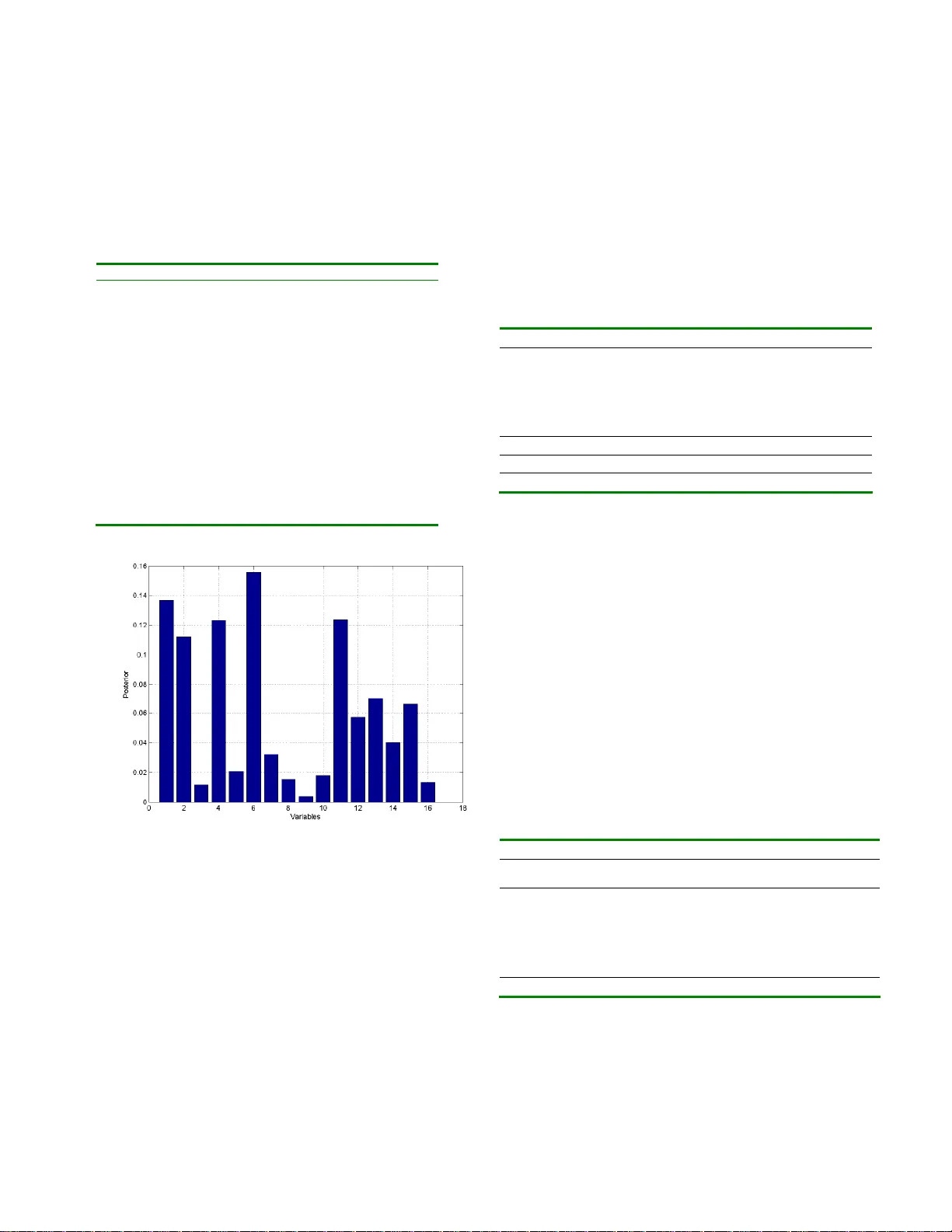
1 Feature Selection for Bayesi an Evaluation of Traum a Death Risk L. Jakaite and V. Schetinin University of Bedfordshire/Department of Computing and Information Systems, Luton, UK Abstract — In the last year more than 70,0 00 people have been brought to the UK hospitals with serious injuries. Each time a clinician has to urgently take a patient through a screening procedure to make a reliable decision on the trauma treatment. Typically, such procedure comprises around 20 tests; however the condition of a trauma patient remains very difficult to be tested properly. What happens if these tests are ambiguously interpreted, and information about the severity of the injury w ill come misleading? The m istake in a decision can be fatal – using a mild treat ment can put a patient at risk of dying from posttraumatic shock, while using an over- treatment can also cause death. How can w e redu ce the risk of the death caused by unreliable decisions? It has been shown that probabilistic reasoning, based on the Bayesian methodol- ogy of averaging over decision models, allows clinician s to evaluate the uncertainty in decision making. Based on this methodology, in this paper w e aim at selecting th e most impor- tant screening tests, keeping a high performance. We assume that the probabilistic reasoning within the Bayesian methodol- ogy allows us to discover new relationships between the screen- ing tests and uncertainty in decisions. In practice, selection of the most infor ma tive tests can also reduce the cost of a screen- ing procedure in trauma care centers. In our experiments we use the UK Trauma data to compare the efficiency of the pro- posed technique in terms of t he performance. We also compare the uncertainty in decisions in terms of entropy. Keywords — Bayesian model averaging, MCMC, decision tree, trauma care, feature selection. I. I NTRODUCTION As it has been reported in [1], more than 70,00 0 people have been admitted into the UK hospitals with serious inju- ries. To make a reliable decisi on on the trau ma treatment, a clinician has to urgently take a patient throu gh a screening procedure which typically compri ses around 20 tests [2]. However, the condition of a trauma patient is still very difficult to be tested prop erly. If the screeni ng tests are ambiguously interpreted, and information about the severity of the injur y is misleading, the mistake in a decision can be fatal; the choice of a mild treatment can put a patient at risk of dying from posttraumatic shock, while the choice of an overtreatment can also cause death [1]. How can we red uce the risk of the death caused b y unreliable decisio ns? It has been shown in [3 - 6] that prob abilistic reasonin g, based on the Bayesian methodology of averaging over deci- sion models, enables to evaluate the uncertainty in decision making. The use of the Ba yesian Model Averaging (BMA) over Decision Tre es (DTs) makes decision models inter - pretable for clinicians as shown in [7]. The Bayesian aver- aging over DTs (BDT s) enables to select attributes which make the most significant contrib ution to decisions. Within the Ba yesian DTs averaging we would expect that discard - ing weakest attributes would improve the performance. However, in our experiments, w e observed that the per- formance decreased. Obviously, we can explain that this happened because the discarded attribute was still important for a small amount of the data. If this is the case, then we can expect that the replacement of this attribute by noise will further decrease the performance. Alternatively, we ca n assume that the weakest attri bute makes a contribution to the BM A. Would it be possible to discard the weakest at- tribute without decreasing the performance? If so, then we can reduce the number of screening tests requir ed for mak- ing reliable decisio ns within BDT methodology. In theory, BMA methodology is immune to overfitting problem [3]. However, in some cases, overfittin g was shown to affect the BM A perfor mance [8]. Based on these results we can assume t hat if the replace ment of the weakest attribute by noise does not decrease the BMA perfor man ce, this attrib ute, making negligib le contribution, provides bet- ter conditions for mitigating B MA overfitting. Based on these assumptions, in this paper we aim at se- lecting the most importa nt screening tests, keeping the BDT performance high. This is important because selection of the most informati ve screening tests can reduce the cost of a screening proced ure in trauma care centers. In our experi- ments we use the UK Trauma data to compare the effi- ciency of the prop osed BMA technique in terms of the per- formance. We also compare the uncertaint y in decisio ns in terms of entrop y. Section 2 of the paper describes the bases of BMA over DTs, and section 3 describes the Trauma data used for the experiments. The experi mental results are presented in sec- tion 4, and section 5 conclude s the paper. II. METHODOLOG Y OF BAYESIAN MODEL AV ERAGING For a DT given with parameters  , the predictive distri- bution is written a s an integral over the para meters  2    θ D θ D θ x D x d p y p y p ) | ( ) , , | ( ) , | ( where y is the predicted class (1, …, C ), x = ( x 1 , …, x m ) is the m -dimensional vector of input, and D are the given training data. This integral can be analyticall y calculated only in si mple cases, and in practice part of the integrand, which is the posterior density of  conditio ned on the data D, p (  |D) , cannot usually be evaluated. However if values  (1) , …,  ( N ) are the samples dra wn from the posterior distribution p (  |D) , we can w rite       N i i i N i i y p N p y p y p 1 ) ( ) ( 1 ) ( ) , , | ( 1 ) | ( ) , , | ( ) , | ( D θ x D θ D θ x D x The above integral can be approximated by using Markov Chain Monte Carlo (MCMC) technique [3]. To perform such an approximation, we need to run a Markov Chain until it has converged to a stationary distribution. Then we can collect N random samples from the posterior p (  |D) to calculate the desire d predictive p osterior density . Using DTs for the classification, we need to find the probability  tj with which an input x is assigned by terminal node t = 1, …, k to the j th cl ass, where k is the number of terminal nodes in the DT. The DT parameters are de fined as  = ( s i pos , s i var , s i rule ), i = 1 , …, k – 1, where s i pos , s i var and s i rule define the position , predictor and rule of each splitting node, respectively. For these parameters the priors can be specified as follows. First we can define a maximal number of splitting nodes, say, s max = n – 1. Second we dra w any of the m predicto rs from a uniform discrete distribution U (1, …, m ) and assign } ,..., 1 { var m s i  . Finally the candidate value for the splitting variable x j = s i var can be drawn from a discrete distribution U ( x j (1) , …, x j ( L ) ), w here L is the number of possible splitting rules for variable x j , either categorica l or continuous. Such priors allow us to explore DT s which split data in as many ways as possible. However the DTs with different numbers of split- ting nodes should be explored in the same p roportions [3]. To sample DTs of a variable dimensionalit y, the MCM C technique exploits the Rever sible Jump extension [3]. To implement the RJ MCMC technique, Denison et al. [3] and Chipman et al. [6] have suggested exploring the posterior probability by using the followin g types of moves: 1. Birth . Randomly split the data points falling in one of the terminal nodes by a new splitting node with the variable and rule dra w n from the correspo nding priors. 2. Death . Randomly pick a splitt ing node with two ter- minal nodes and assign it to be one terminal with the united data p oints. 3. Change-split . Randomly pick a splitting node and assign it a new splitting variable and rule dra wn from the corresponding priors. 4. Change-rule . Randomly pick a splitting node and as- sign it a new rule drawn fro m a given prior. The first two moves, birth and death , are reversible and change the dimensiona lity of  . The remaining moves pro- vide jumps within the current dimensionality o f  . Note that the change-split move is included to make “large” jumps which potentially increase the chance of sampling from a maximal p osterior whilst the change-rule move do es “local” jumps. The RJ MCMC technique starts dra w ing samples from a DT consisting of one splitting node whose para meters were randomly assig ned within the predefined priors. So we need to run the Markov Chain while a DT grows and its likeli- hood is unstable. This phase is said burn-in and it should be preset enough long in order to stabilize the Markov Chain. When the Markov Chain will be enough stable, we ca n start sampling. T his phase is said post burn-in . III. THE PROPOSED METH OD To test the assumptions made in section I, we propose two methods – the first is based on selection of DTs ensem - ble, and the second is based on the rando mization of vari- ables. The selection techniqu e aims to omit the DTs which use the weakest variable. The rando mization technique aims to provide better conditions for mitigating DT ensemble overfitting. In the following sections we test and compare these techniques o n the Trauma data. IV. EXPERI MENTS AND RESULTS A. Trauma Da ta The Tra um a data collec ted at the Royal London Hospita l comprises 16 screening tests and attributes and the outcome (lived or died) for 316 injured patients. Among these vari- ables 5 are continuous and 11 are categorical, see T able 1. B. Variable’ s Importance In our experi ments we collecte d 10,000 DTs during post burn-in phase after sampling 200,000 DTs during burn-in phase. The sampling rate for post burn-in phase was 7; the 3 number of minimal data instances allowed in DT nodes w as 3; the acceptance rate was around 0 .25. Having obtai ned the ensembl e of DTs, we estimated the importance of all 16 variables for the predictio n. The esti- mates were calculated as the posterior probabilities of vari- ables used in the DT s ensemble as shown in Fig. 1. Table 1 Scree ning tests and attributes of the Trauma data No Screening Tests and Attrib utes Type 1 Age Continuous 2 Gender: Male = 1, Fe male = 0. 0,1 3 Injury type: Blunt = 1, penetra ting = 0 0,1 4 Head injury , no injury = 0 0,1,2,3,4,5,6 5 Facial injury 0,1,2,3,4 6 Chest injury 0,1,2,3,4,5,6 7 Abdominal or pelv ic contents injury 0,1,2,3,4,5 8 Limbs or bony pelv is in jury 0,1,2,3,4,5 9 External injury 0,1,2,3 10 Respiration rate Continuous 11 Systolic blood pressure Continuous 12 Glasgow coma score (G CS) eye response 0,1,2,3,4 13 GCS motor response 0,1,2,3,4,5,6 14 GCS verbal re sponse 0,1,2,3,4,5 15 Oximetry Continuous 16 Heart rate Continuous 17 Died = 1, living = 0. 0,1 Fig. 1 Posterior probabil ities of variables used in the ense mble From Fig. 1 we can observe that the posterior probability of variable 9 is the smallest, around 0.005 , while the maxi- mal value is around 0.16 for variable 6. Therefore w e can assume that the variable 9 makes negligible contribution to the ensemble’s outcome. To test our assumptions, we aim to discard this variable from the T rauma data. Tab le 2 shows the maximal values o f loglikelihoods calculated within 5- fold cross-validation for two sets includin g 16 and 16\9 variables. From this table, we can observe that the logli kelihood value for the 16\9 set becomes greater than that for the set of all 16 variables. However the per formance of the ensemble using the set of 16\9 variables is slightly fewer than that using the set of 16 variables. This can happen because the ensemble using the set of 16\9 variab les bec omes more over fitted to the training data. Thus, w e can conclude that the w eakest variable 9 provides better conditions for mitigating the DT ensemble overfitting. Table 2 Maximal logl ikelihoods, L 16 and L 16\9 , performances and entrop ies of the ensembles using sets of 16 and 16\9 variable s within 5-fold cross- validation Fold Loglikelihood ( L 16 ) Loglikelihood ( L 16\9 ) 1 -36.14 -33.4 2 -44.29 -37.33 3 -37.23 -33.19 4 -36.24 -38.37 5 -37.98 -40.41 Loglikelihood -38.37 ±3.39 -36.48 ±3.23 Performance, % 84.66 ±4.70 83.85 ±6.95 Entropy 29.8 ±2.1 30.0 ±4.7 C. Selection of DT Ensemb le As shown above, the presence of the weakest variable has the positive effect on mitigating overfitting of the DT ensemble. This means that the DT ensemble should use all 16 input variables duri ng sampling, b ut then we can e xclude those DTs w hich use the weakest variable 9. After such selection of DTs there is no ne ed to use the variable 9. In our experiments this technique was tested within 5- fold cross-validation and results shown in Tab le 3 which compares the perfor mance of the original DT ensemble using all 16 variables with the performance of the selected ensemble. This table also shows the number of DTs omitted after the selection. Table 3 Perf ormances and entropies of the original and selected ensembles within 5-fold cross-val idation Original ensemble Selected ensemble Fold Performance, % Entropy BDTs omitted Perform ance, % Entropy 1 85.93 26.47 314 85.93 26.46 2 80.95 28.89 467 80.95 28.91 3 84.13 31.80 217 84.13 31.79 4 82.54 32.05 631 82.54 32.04 5 87.30 31.44 336 87.30 31.46 84.17±2.54 30.13±2.40 393±160 84.17±2.54 30.13±2.40 This table show that the performance of the selected ensemble using 16\9 variables is the same as that of the 4 original ense mble using all 16 input variables. The entropies in decisions are also the same. Thus from this experiment we can see that prop osed technique allows us to use a re- duced set of variables. D. Addition of Noise to Variables In our experiments some amount of noise added to a weak variable can provide better conditions for mitigating DTs ensemble overfitting. Therefore, we can assume that the addition of noise to all variables will further improve conditions for mitigating DTs ensemble overfitting. To test this assumption we removed the variable 9 and added a uniform noise to the remaining 15 variables. The intensity of the noise was 0.01. Table 4 shows the perfor m- ances of DT ensembles using the set of 16 variables and the set of 16\9 with the added noise compared within 5-fold cross-validation. This table shows that the perfor mance of the DT ensemble using the set of 16\9 + noise is better on 2%, than that of the ense mble using the original 16 inputs. Table 4 Perform ance and entropy of the ensemble s using 16 variables and 16\9 variables with noise e stimated within 5-fol d cross-validation Fold Trauma (16 variables) Trauma (16\9 variable s + noise) Performance, % Entropy Performance, % Entropy 1 84.37 26.63 85.93 26.52 2 79.36 28.70 80.95 30.31 3 84.12 32.54 88.88 32.47 4 88.88 31.24 90.47 32.00 5 88.88 28.11 88.88 32.65 85.13± 7.94 29.4± 4.80 87.03± 7.54 30.8± 5.10 Thus we can see that the addition of the noise to the set of 16\9 variables allows us to exclude the weakest variable 9 and, at the same time, this enables to improve the DT en- semble perfor mance. V. CONCLUSIONS & DISCUSSION We have expected that discar ding weakest attributes can improve the perfor mance of the BDT ensemble. However, in our experiments, the perfor mance has oppo sitely de- creased. We have assumed that this happened because the discarded weakest attrib ute was still importa nt for a small amount of the data. Alternatively, we have assumed that the weakest attrib ute makes a noticeable contribution to the BDT ensemble’s outcome. The question was would it be possible to discard the weakest attribute without decreasi ng the perfor man ce? This is important for clinical practice if the number of screening tests required for making reliable decisions within BDT methodo logy can be reduced . Although BM A methodolo gy in theor y is immune to overfitting prob lem, in some cases, it was shown that over- fitting affects the BMA performance. We have observed that the replace ment of the weakest attribute by noise did not decrease the BDT performance, and therefore this at- tribute, making negligible contribution, provided better conditions for mitigating BDT ensemble overfitti ng. In this paper w e aimed at selecting the most important screening tests, keeping the BDT performance high. In our experiments we used the UK Trauma data to compare the efficiency of the proposed technique in terms of the per- formance. We also compare the uncertaint y in decisio ns in terms of entrop y. As a result we found that the prop osed techniques allow clinicians to reduce number of screening tests, keeping the performance and reliability of making decisions high. The optimized solutions can reduce the cost of a screening pro- cedure in trauma care centers. R EFERENCES 1. Royal Society for the Prevention of Accidents available at http://www .rospa.com/factsheets 2. Trauma Audit and Research Netw ork available at http://www .tarn.ac.uk 3. Denison D, Holmes C, Malick B, Smith A (2002) Bayesian methods for nonlinear classification and regression. Willey 4. Breiman L, Friedman J, Olshen R, Stone C (1984) Classific ation and regression trees. Bel mont, CA: Wadsw orth. 5. Buntine W (1992) Learning classification trees. Statistics and Com- puting 2: 63-73 6. Chipman H, George E, McCullock R (1998) Bayesian CART model search, J. American Statis tics, 93: 935-960 7. Schetinin V et al. (2007) Confident Interpretation of Bayesian Deci- sion Trees for Clinical Applications. IEEE Transaction on Informa- tion Technology in Biome dicine, Volume 11, I ssue 3, 312-319 8. Domingos P (2000) Bayesian Averaging of Classifiers and the Over- fitting Problem, Proc. 17th International Conf. on Machine Learning, San Francisco, CA, 2000, 223-230 Author: L Jakaite Institute: University of Bedfordshire Street: Park Square City: Luton Country: UK Email: Livija.Jakaite@gmail.com