Estimation of Large Precision Matrices Through Block Penalization

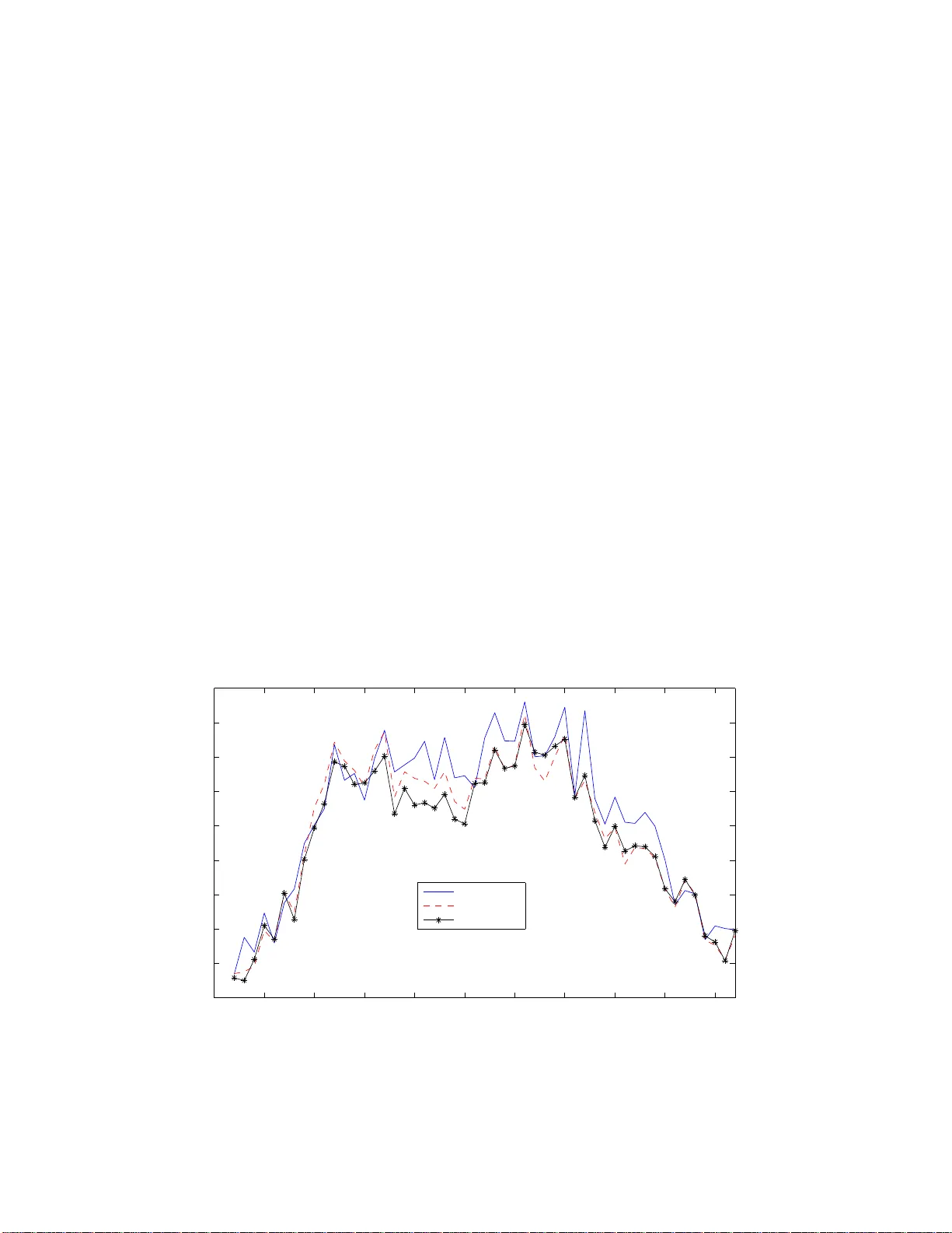
Estimation of Large Precision Matrices Through Blo c k P enalization ∗ By Cliffor d Lam Department of Op er atio n s Resea r c h a nd Financi al Eng i neering Princet o n Universit y , Princeto n, NJ, 0 8544 This pap er fo cuses on exploring the sparsit y of the in v erse cov ariance ma- trix Σ − 1 , or t he precision matrix. W e form blo c ks of parameters based on eac h off-diagonal band of the Cholesky factor fro m its mo dified Cholesky decomp osition, and p enalize eac h blo ck of parameters using the L 2 -norm in- stead of individual elemen t s. W e dev elop a one-step estimator, and pro ve an oracle prop erty whic h consists of a notion of blo ck sign-consistency and asymptotic normalit y . In particular, pro vided the initial estimator o f the Cholesky factor is go o d enough and the true Cholesky has finite n um b er of non-zero off-diagonal bands, or a cle property holds for the one-step estimator ev en if p n ≫ n , and can ev en b e a s large as log p n = o ( n ), where the data y has mean zero and tail probability P ( | y j | > x ) ≤ K exp( − C x d ), d > 0, and p n is the n um b er o f v ariables. W e also pro ve an op erat or norm conv ergence result, sho wing the cost of dimensionalit y is just log p n . The adv an tage of this method o ve r banding b y Bic k el and Levina (200 8) or nested LASSO b y Levina et al. (2007) is that it allo ws f or eliminatio n of w eake r signals that precede stronger ones in the Cholesky factor. A method for obtaining an initial estimator for the Cholesk y factor is discus sed, and a gradien t pro jec- tion algorithm is dev elop ed for calculating the one- step estimate. Sim ulation results are in fav or o f t he new ly pro p osed metho d a nd a set of real data is analyzed using the new pro cedure and the banding method. Short Title : Blo c k-p enalized Precision Matrix Estimation. AMS 2000 subje ct class ific ations . Primary 62F12; secondary 62H12. Key wor ds and phr ases . Co v aria nce matrix, high dimensionalit y , mo dified Cholesky decomp osition, blo c k p enalt y , blo c k sign-consistenc y , ora cle property . ∗ Clifford La m, PhD studen t (Email: wlam@princeton.edu. Phone: (60 9) 240- 6 928). Financial sup- po rt from the NSF grant DMS-07 04337 and NIH grant R01-GM0726 11 is gr atefully ackno wledged. 1 1 In tro ductio n The need for estimating large co v ariance matrices arises naturally in many scien tific applications. F or example in bioinformatics, clus tering of genes using genes expression data in a microarray exp erimen t ; or in finance, when seeking a mean-v ariance efficien t p ortfolio from a univ erse of sto ck s. One common feature is that the dimension of the data p n is usually large compare with the sample size n , or ev en p n ≫ n (genes exp ression data, fMRI data, financial da t a , among man y others). The sample co v ariance matrix S is w ell-kno wn to b e ill-conditioned in suc h cases. Ev en for Σ = I the iden tit y matrix, the eigen v alues of S ar e more spread o ut ar ound 1 asymptotically as p n /n gets larger (the Mar ˆ cenk o-Pastur law, Marˆ c enk o and P astur, 1967). It is singular when p n > n , thus not allo wing a n estimate of the in v erse o f the co v ariance mat r ix, whic h is needed in many m ultiv aria te statistical pro cedures lik e t he linear discriminan t analysis (LD A), regression for mu ltiv ariate norma l data, Gaussian gra phical models or p ortfolio allo cat io ns. Hence alternativ es are needed for more accurate and useful estimation o f cov ariance matrix. One regularization approa c h is p enalization, whic h is the ma in fo cus o f this pa p er. Sparse estimation of the precision mat r ix Ω = Σ − 1 has b een in v estigated by man y r e- searc hers, whic h is v ery useful in Ga ussian graphical mo dels or cov ariance selection for naturally ordered da ta (e.g. long itudinal data, see Diggle and V erb yla (19 98)). Mein- shausen and B ¨ uhlmann (20 06) used the L 1 -p enalized lik eliho o d to c ho ose suitable neigh- b orho o d for a Gaussian graph and show ed that p n can grow arbitrarily fast with n for consisten t estimation, while Li and Gui (2006) considered up dating the off- diagonal ele- men ts o f Ω b y p enalizing on the negative gradien t of the log- likelihoo d with resp ect to these elemen ts. Banerjee, d’Aspremon t and El Gha oui (2006) and Y uan a nd Lin (20 07) used L 1 -p enalt y to directly penalize on the eleme n ts of Ω , and dev elop differen t semi- definite programming alg o rithms to ac hiev e sparsit y of the in v erse. F riedman, Hastie and 2 Tibshirani (2 007) and Rothman et al. (2007) considered maximizing the L 1 -p enalized Gaussian log -lik eliho o d on the off-diagonal elemen ts of the precision matrix Ω , where the Graphical LASSO and the SPICE algorithms are prop osed resp ectiv ely in their pap ers for finding a solution, and the latter pro ved F ro b enius and op erator norms con v ergence results for t he final estimators. P oura hmadi (1 9 99) prop osed the modified Cholesky decomp osition (MCD) whic h fa- cilitates greatly the sparse estimation of Ω t hr o ugh p enalization. The idea is to decomp ose Σ suc h that for zero-mean data y = ( y 1 , · · · , y p n ) T , we ha v e for i = 2 , · · · , p n , y i = i − 1 X j = 1 φ i,j y j + ǫ i , and TΣT T = D , (1.1) where T is the unique unit lo we r triangular matrix with ones on it s diagona l and ( i, j ) th elemen t − φ i,j for j < i , and D is diago na l with i th elemen t σ 2 i = v ar( ǫ i ). The optimization problem is unconstrained (since the φ ij ’s are free v ariables), and the estimate fo r Ω is alw ays p ositive -definite. With MCD in (1.1), Huang et al. (2 006) used the L 1 -p enalt y on the φ i,j ’s and optimized a p enalized G aussian log-lik eliho o d through a prop osed iterativ e sc heme, with the case p n < n considered. Levina, Rothman and Zhu (200 7) pr o p osed a no ve l p enalty called the nested LASSO to ac hiev e a flexible banded structure of T , and demonstrated b y sim ulations t ha t norma lity of data is not necessary , with p n > n considered. F or estimating the precision matrix Ω for naturally ordered data, a pa rt f r om the nested LASSO, Bick el and Levina (200 8) prop osed banding the Cholesky factor T in (1.1), with the banding order k chose n by minimizing a resampling-based estimation of a suitable risk measure. The metho d w orks on estimating a co v aria nce matrix as w ell. While these tw o metho ds are simple to use, t hey cannot eliminate blo cks of w eak signals in b et we en stronger signals. F or instance, consider a time series mo del y i = 0 . 7 y i − 1 + 0 . 3 y i − 3 + ǫ i , 3 whic h corresp onds to (1.1) with φ i, 2 = 0, φ i,j = 0 for j ≥ 4. F or example, this kind of mo del can arise in clinical tria ls data, where response o n a drug f o r pat ients follo ws a certain kind of autoregressiv e pro cess with w eak signals preceding stronger ones. This implies a banded Cholesky factor T , with the first and t hird off-diagonal bands b eing non-zero and zero otherwise. Banding and nested LASSO can band the Cholesky factor T starting from the fourth off-dia g onal ba nd, but cannot se t the second off-diagonal band to zero. And if these metho ds c ho ose to set the second off-diagonal band to zero, then the third non-zero off-diagonal band will b e wrongly set to zero. Both failures can lead to inaccurate a nalysis or prediction, in particular the maxim um eigenv alue of a precision matrix can then b e estimated v ery wrongly . Clearly , an alternativ e metho d is required in this situation. W e presen t the blo ck penalization fr amew ork in the next section and more motiv a t ions and details of the methodo logy . F or more references, Smith and Kohn (20 0 2) used a hierarchic al Ba y esian mo del to iden tify the zeros in the Cholesky factor T of the MCD. F an, F an and Lv (2007), using factor analysis, dev elop ed high-dimensional estimators fo r b oth Σ and Σ − 1 . W u and P oura hmadi (2003) prop o sed a banded estimator through smoot hing of the lo w er off- diagonal bands of ˆ T obtained from the sample co v ariance matr ix (implicitly , p n < n ). Then an order for banding of ˆ T is c hosen b y using AIC p enalty of normal lik eliho o d of data. F urrer and Bengtsson (2007) considered gradually shrinking the off- diagonal bands’ elemen ts of the sample co v ariance matr ix tow ards zero. Bick el and Levina (2007) and El Ka roui (20 07) prop osed the use of en try-wise thresholding to ac hiev e sparsit y in co v ar ia nce matrices estimation, and pro v ed v arious asymptotic results, while Rothman, Levina and Zh u (2 0 08) generalizes these results to a class o f shrink age op erators whic h includes man y commonly used p enalty functions. W ag aman and Levina (2007) deve lop ed an algorithm for finding a meaningful ordering of v aria bles using a manifold pro jection tec hnique called the Isomap, so that exis ting metho d lik e banding can be applied. 4 The rest of the pap er is orga nized as follow s. In section 2 , w e introduce the mo del for blo c k p enalization, and the motiv ation b ehind. A notion of sign-consistency , w e name it blo c k sign- consistency , is in tro duced. T ogether with asymptotic normalit y , w e call it the oracle prop ert y of the resulting one-step estimator. An initial estimator needed for the one-step estimator, with the blo ck zero-consistency concept, is in tro duced in section 2.5. A practical algorithm is discussed, with sim ulations and r eal data analysis in section 3. Theorems 2(i) and 3 are prov ed in the App endix, whereas Theorems 2(ii) and 4 are pro v ed in the Supplemen t. 2 Blo c k P en ali z ation F ramew ork 2.1 Motiv ation F or data with a natural ordering of the v ariables, e.g. longitudinal data, or data with a metric equipp ed lik e spatial data with Euclidean distance, if dat a p oints are remote in time or space, they are likely to ha ve w eak o r no correlation. Then T in equation ( 1.1), and thus Ω , are banded. Banding and neste d LASSO men tioned in se ction 1 are based on this observ ation for obtaining a banded structure of the Cholesky factor T . See Figure 1(b) for a picture of a banded Cholesky factor. Also, for v aria bles within a close neigh b orho o d, the dep endence structure should be similar. Equation (1.1) then sa ys that co efficien ts on a n off-diagona l band o f the Cholesk y factor T are close to neighboring co efficien ts (see also W u and P oura hmadi (20 0 3)). This means that we can impro v e our estimation if we can efficien tly use neigh b orho o d infor- mation (along a n off-diagonal band of T ) to estimate the v alues of individual co efficien ts. With these insigh ts, w e are motiv ated to use the blo c k p enalization metho d. In the con t ext of w av elet co efficie n ts estimation, Cai (1999) in tro duced a James-Stein shrink age 5 rule o v er a blo c k of co efficien ts, whereas Antoniadis and F a n (20 01, page 966 ) w ere the first to p oint out that suc h metho d can b e regarded as a sp ecial kind of p enalized lik eliho o d whic h p enalizes on the L 2 norm of a group of co efficien ts, a nd in tro duced a separable blo ck -p enalized least squares for simple solutions. Both pap ers arg ue that blo c k thresholding helps pull information from neigh b oring empirical w av elet co efficien ts, th us increasing the information a v ailable for estimating co efficien ts within a blo ck . Y uan and Lin (2006) intro duced the same metho d, whic h they called the group LASSO, to select group ed v ar ia bles (facto r s) in m ulti- f actor ANOV A and compare group ed v ersion of LARS and LASSO. Z ho u, Ro c ha and Y u (2007) further introduced a p enalt y called the Composite Absolute P enalty (CAP) to in tro duce grouping and a hierarc h y at the same time for the estimated parameters in a linear mo del. Blo c k p enalization allo ws for a flexible banded structure in T since zero o ff-diagonal bands can precede the non-zero ones. This is an adv an tage ov er banding of Bic k el and Levina (2008) and nested LASSO o f Levina et al. (2007) as discussed in section 1 . Moreo v er, the blo c k sign-consistency prop erty in Theorem 2(i) implies a banded estimated Cholesky factor T if the truth T 0 is banded. See Figure 1 for a demonstration. Figure 1 : Pattern of zer os in the r esulting estimator for T using (a)Blo ck Penaliza tion ; (b)Banding; (c)Neste d LASSO; (d)LASSO 6 2.2 Blo c k p enalization As p ointed out in Levina et al. (2007), the MCD in (1.1) do es not require the normalit y assumption of the data, and t hey in tro duce a least squares v ersion for their p enalization. W e also use suc h an approach , and define L n ( φ n ) = n X i =1 p n X j = 2 ( y ij − y T i [ j ] φ j [ j ] ) 2 , (2.1) with y i [ j ] = ( y i 1 , · · · , y i,j − 1 ) T , φ n = ( φ T 2[2] , · · · , φ T p n [ p n ] ) T , a nd φ j [ j ] = ( φ j, 1 , · · · , φ j,j − 1 ) T . When p λ n ( · ) is singular at the origin, the term-b y-term p enalt y P p n i =2 P i − 1 j = 1 p λ n ( | φ i,j | ) has its singularit ies lo cated at eac h φ i,j = 0, and the blo c k p enalt y J ( φ n ) = p n − 1 X j = 1 p λ nj ( k ℓ j k ) , (2.2) has its singularities lo cated at ℓ j = 0 for j = 1 , · · · , p n − 1, where λ nj = λ n ( p n − j ) 1 / 2 , ℓ j = ( φ j + 1 , 1 , φ j + 2 , 2 , · · · , φ p n ,p n − j ) T is the j th off-diagonal band of the Cholesky factor T in (1.1), and k · k is the L 2 v ector norm. Hence t his blo c k p enalt y either kills off a whole off-diagonal band ℓ j or k eeps it en tirely (see also Antoniadis and F an (2001)). Com bining (2.1) and (2.2) is the block-penalized least squares Q n ( φ n ) = L n ( φ n ) + nJ ( φ n ) . (2.3) W e will use the SCAD p enalt y function for p λ ( · ) in (2.2), defined through its deriv ative p ′ λ ( θ ) = λ 1 { θ ≤ λ } + ( aλ − θ ) + 1 { θ>λ } . (2.4) SCAD p enalty is an un biased p enalt y function whic h has theoretical adv an tages ov er L 1 -p enalt y (LASSO). See Lam and F an (20 0 7) for more details. In fact, in F an, F eng and W u (2007), the SCAD-p enalized estimate o f a gr aphical mo del is substan tially sparser than the L 1 -p enalized one, which has spuriously large num b er of edges, partially due to 7 the bias induced b y L 1 -p enalt y and hence requiring a smaller λ that induces spurious edges. With ˆ φ n , we estim ate D in (1.1) b y ˆ σ 2 1 = n − 1 n X i =1 y 2 i 1 , ˆ σ 2 j = n − 1 n X i =1 ( y ij − y T i [ j ] ˆ φ j [ j ] ) 2 , j = 2 , 3 , · · · , p n . (2.5) 2.3 Linearizing the SCAD p enalt y Minimizing Q n ( φ n ) in (2 .3) poses some c hallenges. Firstly , Q n ( φ n ) is not separable, whic h makes our problem computationally c hallenging. Secondly , the SCAD p enalt y complicates the computations as there are no easy simplifications of the problem lik e equation (5) in Antoniadis a nd F an (2001, page 966). Zou and Li (2 0 07) show ed that linearizing the SCAD p enalty leads t o efficien t algo- rithms like the LARS to b e applicable, and that sparseness, unbiasedne ss and con tin uit y of the estimators contin ue to hold (see F an and Li (2001)). F ollow ing their idea, we linearize each p λ nj ( k ℓ j k ) in (2.2) at an initial v alue k ℓ (0) j k so that minimizing (2.3) is equiv alent to minimizin g, fo r k = 0 , Q ( k ) n ( φ n ) = n X i =1 p n X j = 2 ( y ij − y T i [ j ] φ j [ j ] ) 2 + n p n − 1 X j = 1 p ′ λ nj ( k ℓ ( k ) j k ) k ℓ j k , (2.6) where w e denote the resulting estimate by φ ( k +1) n . P arallel to Theorem 1 and Prop osition 1 of Zou and Li (2007), w e state the following theorem concerning conv ergence in iterating (2.6) starting from k = 0. Theorem 1 F o r k = 0 , 1 , 2 , · · · , the a s c ent pr op erty holds for Q n w.r.t. { φ ( k ) n } , i.e . Q n ( φ ( k +1) n ) ≥ Q n ( φ ( k ) n ) . F urthermor e, let φ ( k +1) n = M ( φ ( k ) n ) , so that M is the map c arrying φ ( k ) n to φ ( k +1) n . I f Q n ( φ n ) = Q n ( M ( φ n )) only for stationary p oints of Q n and if φ ∗ n is a limit p oint of the se quenc e { φ ( k ) n } , then φ ∗ n is a stationary p oint Q n . 8 This con v ergence result follows from more general conv ergence results for MM (minorize- maximize) algo rithms. Hence starting from a n initial v alue φ (0) n , w e ar e able to it- erate (2.6) to find a stationary po in t of Q n . Note that ev en starting from the most primitiv e initial v alue φ j [ j ] = 0 , the first step g iv es a group LASSO estimator since p ′ λ nj (0) = λ nj = λ n ( p n − j ) 1 / 2 . Hence the second step gives a biased reduced estimator of LASSO, as p ′ λ nj ( k ℓ ( k ) j k ) = 0 for k ℓ ( k ) j k > aλ nj . In section 2.5 w e sho w ho w to find a go o d initial estimator whic h is t heoretically sound, and iterating until conv ergence is not alw ays neede d. 2.4 One-Step Estimat or for φ n W e no w dev elop a one-step estimator to reduce the computational burden a nd pro ve that suc h an estimator enjo ys the oracle prop ert y in Theorem 2. The p erformance of this one-step estimator dep ends o n the initial estimator φ (0) n . D efine, for ℓ j 0 denoting the true v alue of ℓ j in T , J n 0 = { j : ℓ j 0 = 0 } , J n 1 = { j : ℓ j 0 6 = 0 } . Definition 1 An initial estimator φ (0) n is c al le d blo ck zer o-c onsistent if ther e exists γ n = O (1) such that (a) P  max j ∈ J n 0 k ℓ (0) j k / ( p n − j ) 1 / 2 ≥ γ n  → 0 as n → ∞ , and (b) for the same γ n , P  min j ∈ J n 1 k ℓ (0) j k / ( p n − j ) 1 / 2 ≥ γ n  → 1 . This definition is similar to the idea of zero- consistency intro duced in Huang, Ma and Zhang (2 0 06), but w e now define it at the blo ck lev el, whic h concerns the av erage magnitude of each elemen t in the off-diagonal ℓ (0) j . With this, w e presen t the main theorem of this section, the oracle prop ert y f o r the one-step estimator. Theorem 2 Assume r e gularity c onditions (A) - (E) in the App en dix, and the Cholesky factor T 0 of the true pr e cision matrix Ω 0 has k n < n non-zer o off-diagona l b ands. If the 9 initial estimator φ (0) n for Q (0) n in (2.6) is blo ck zer o-c onsistent, then the r esulting estimator ˆ φ n by minim izing (2.6) satisfies the fol lowing: (i) (Blo ck sign-c onsistency) P ( A ∩ B ) → 1 , wher e A = { ˆ ℓ j = 0 for all j ∈ J n 0 } , and B = { sgn( ˆ φ j + k, k ) = sgn( φ 0 j + k, k ) for all j ∈ J n 1 , k so that φ 0 j + k, k 6 = 0 } . (ii) (Asymptotic norma lity) L et φ n 1 b e the ve ctor of elements of φ n c orr esp onding to its no n-zer o off- d iagonals. Then for a ve ctor α n of the same size as ˆ φ n 1 so that α n has at most k n non-zer o elements and k α n k = 1 , if k 4 n (log 2 ( k n + 1 ) ) 4 /d /n = o (1) , we have n 1 / 2 ( α T n H n α n ) − 1 / 2 α T n ( ˆ φ n 1 − φ 0 n 1 ) D − → N (0 , 1) , wher e H n is blo ck diagon a l wi th p n − 1 blo cks. Its ( j − 1) -th blo ck is σ 2 j 0 Σ − 1 j 11 , and Σ j 11 = E ( y i [ j ] (1) y i [ j ] (1) T ) , wher e y i [ j ] (1) c o n tains the elements of y i [ j ] c orr esp onding to the n o n - zer o off-diag onals’ elements of φ 0 j [ j ] . F rom this theorem and regularity condition (C) in the App endix, the size p n of the co v ar ia nce matrix can b e la r ger than n . In particular, if k n is finite, the oracle pro p ert y still holds when log p n = o ( n ). This is useful for many a pplications with p n > n , when the sample co v ariance matrix b ecomes singular, whereas Theorem 3 shows that as long as the Cholesky factor is sparse enough, we can get an optimal estimator of the precision matrix via penalization. Theorem 3 L et ˆ T b e the one-s tep es timator as in The or e m 2, and ˆ D b e diagonal with elements ˆ σ 2 j as define d in (2.5), so that ˆ Ω = ˆ T T ˆ D − 1 ˆ T . Then under r e gularity c o nditions (A) - (E) in the App endix, with Ω 0 denoting the true pr e cision matrix, k ˆ Ω − Ω 0 k ∞ = O P (( k n + 1) 3 / 2 (log p n /n ) 1 / 2 ) , k ˆ Ω − Ω 0 k = O P (( k n + 1) 5 / 2 (log p n /n ) 1 / 2 ) , wher e k M k ∞ = max i,j | m i,j | , and k M k = λ 1 / 2 max ( M T M ) . 10 W e will demonstrate related num erical results in section 3. F r o m this theorem, the metho d of blo c k penalizatio n allo ws for consisten t precision matrix estimation as long as the cost of dimensionalit y log p n satisfies ( k n + 1) 5 log p n /n = o (1). In particular, if k n is finite, w e only need log p n /n = o (1) f or consisten t estimation. On the ot her hand, pro vided the cost of dimensionalit y is not to o larg e (e.g. p n = n a for some a > 0, so log p n = a log n and is negligible), w e need k n = o ( n 1 / 3 ) for elemen t -wise consistency . 2.5 Blo c k zero-consisten t initial estimat or W e need a block zero- consisten t initial estimator for finding a n oracle one-step estimator in the sense of Theorem 2 . The next theorem show s that the OLS estimator ˜ T , where the sample co v ariance matrix is S = ˜ T − 1 ˜ D ( ˜ T − 1 ) T using the MCD in (1.1), is block zero- consisten t when p n /n → const. < 1. When p n > n , S is singular and ˜ T is not defined uniquely . Since w e en visage a banded t r ue Cholesky factor T 0 with most non-zero off- diagonals close to the diago nal, w e define ˜ T by considering the least square estimators of the regression y i = i − 1 X j = c ni φ i,j y j + ǫ i , (2.7) where c ni = max {⌊ i − γ n ⌋ , 1 } with some constan t 0 < γ < 1 con trolling the n umber of y j ’s on which y i regresses. The rest o f the φ i,j ’s are set to zero, recalling that eve n starting from the most primitiv e initial v alue φ j [ j ] = 0 , t he one-step estimator is a gro up LASSO estimator since p ′ λ nj (0) = λ nj = λ n ( p n − j ) 1 / 2 . Theorem 4 Assume r e gularity c onditions (A) to (E) in the App e ndix. Then the estima- tor ˜ T obtain e d thr ough the ab ove series of r e gr e ssions is blo ck zer o-c onsistent, pr ovid e d al l the true non-zer o off- diagonal b ands of T 0 ar e within the first ⌊ γ n ⌋ off-diagon a l b ands fr om the main diagonal of T 0 . 11 R emark : In high dimensional mo del selection, the condition of “irrepresen t a bilit y” from Zhao a nd Y u (2 0 06), “w eak partial orthogonalit y” from Huang et al. (2006) or the UUP condition fro m Cand ` es and T ao (2007 ) all desc rib e the need of a w eak asso ciation b et w een the relev ant co v ariat es and the irrelev an t o nes under the true mo del, for the estimation procedures to pic k up the correct sparse signals asymptotically . In our case, with (1.1) as the true mo del, the asso ciation b et w een the v ariables y i and y 1 , · · · , y i − 1 for i = 2 , · · · , p n is incorp orated in to the tail assumption of the y ij ’s, whic h is sp ecified in regula r it y condition (A). This assumption en ta ils that the | φ i,j | ’s f o r i and j far apart are small, so that the asso ciation b et w een the relev ant y i ’s (corr. t o φ t,i 6 = 0) a nd the irrelev a nt y j ’s (corr. to φ t,j = 0) in mo del (1.1) ar e small. In practice, for the series of regression described, w e can con t inue to regress y i on the next ⌊ γ n ⌋ y j ’s etc until all the ˜ φ i,j ’s are obtained. W e adapt this initial estimator in the n umerical studies in section 3. Also in practice, the rate a t whic h max j ∈ J n 0 k ℓ (0) j k / ( p n − j ) 1 / 2 con verges to zero in probabilit y in definition 1 ma y not b e fast enough for the OLS estimators. O ne wa y to improv e the qualit y of the OLS estimators is to smooth along the o ff-diagonals o f ˜ T . F or instance, W u and Pourahmadi (2003) smo othed along off- diagonals of the OLS estimator ˜ T t o r educe estimation errors. This amoun ts to assuming that the co efficien ts φ i,i − j = f j,p n ( i/p n ), where f j,p n ( · ) is a smooth function defined on [0 , 1]. W e then c alculate the smoo t hed co efficien ts ¯ φ j + k, k = p n − j X r =1 w j ( r + j, k + j ) ˜ φ j + r ,r , where the we igh ts w j ( r + j, k + j ) dep ends on the smo othing metho d. W e use lo cal p olynomial smo o thing with bandwidth h → ∞ with h/p n → 0, so t ha t v ar( ¯ φ j + k, k ) = O ( n − 1 h − 1 ) (See W u and P ourahmadi (2003) and F a n and Zhang (2000) for more details.). 12 2.6 Algorithm for practical implemen tation Y ua n and Lin (2006) prop osed a group LASSO alg o rithm to solve problems similar to (2.6). Ho wev er, when p n is large, the algo rithm is computationally v ery exp ensiv e. In- stead, w e adapt an idea from Kim, Kim and Kim (2006) and use a gradien t pro jection metho d to solve for the one-step estimator, whic h is computat io nally m uc h less demand- ing. Since minimizing (2.6) can b e considered as a w eigh ted blo c k-p enalized least squares problem with w eigh ts w k nj = np ′ λ nj ( k ℓ ( k ) j k ) /λ n , it can b e formu lated as: minimizing L n ( φ n ) sub ject to s n X j = 1 w k nj k ℓ j k ≤ M (2.8) for some M ≥ 0. Since the further off-diagonal bands of ˜ T are to o short, in practice w e stac k them t o gether until it is of length of order p n . W e then treat it as one blo ck in the ab o v e dual-like problem, and denote b y s n the n um b er of off-diagonals in ˜ T after stac king. Assume for now t hat all the tuning parameters are know n. Starting from an initial v alue φ (0) n and t = 1, the gradien t pro jection metho d in v olv es computing the gra dient ∇ L n ( φ ( t − 1) n ) and defining b = φ ( t − 1) n − s ∇ L n ( φ ( t − 1) n ), where s is t he steps ize of it erat ions to b e f o und in the next section. Denote b y b ( j ) the j th blo c k of b , with blo c ks formed according to t he off-diagona ls ℓ j of T , j = 1 , · · · , s n . Then the main step o f the algorithm is to solv e φ t n = argmin φ n ∈B k b − φ n k 2 , with B = n s n X j = 1 w k nj k ℓ j k ≤ M o , whic h is called the pro jection step. It can b e easily reform ulated as solving min M j s n X j = 1 ( k b ( j ) k − M j ) 2 sub ject t o s n X j = 1 w k nj M j ≤ M , M j ≥ 0 , (2.9) where then ℓ t j = M j b ( j ) / k b ( j ) k , and w e iterate the ab ov e un til conv ergence. Standard LARS or LASSO pac k ages can solv e (2.9) easily , but w e adapt a pro jection algorithm 13 b y Kim et al. (2006) whic h can solv e the ab ov e ev en faster. In solving (2.9), w e are essen tially pro jecting ( k b (1) k , · · · , k b ( s n ) k ) onto the h yp erplane P s n j = 1 w k nj M j = M with M j ≥ 0. The key observ a tion is that if suc h pro jection has non-p ositiv e v alues on some M j ’s, then the solution t o (2.9) should ha v e those M j ’s exactly equal zero. Hence we can then recalculate the pro jection on to the reduced h yp erplane un til no more negativ e v alues o ccur in the pro jection, and it is easy to see that at most s n suc h iterations ar e needed to solv e (2.9). In detail, w e start a t τ = { 1 , · · · , s n } , and calculate the pro jection M j = 1 { j ∈ τ } h k b ( j ) k +  M − X r ∈ τ w k nr k b ( r ) k  w k nj / X r ∈ τ ( w k nr ) 2 i (2.10) for j = 1 , · · · , s n . W e then update τ = { j : M j > 0 } and calculate the ab ov e pro jection again un til M j ≥ 0 for all j . 2.7 Choice of tuning parameters There ar e three tuning parameters introduced in the previous section, namely λ n , M and s . The small n umber s is a parameter for the gra dient pro j ection algorithm and it is re- quired that s < 2 /L , where L is the Lip c hitz constan t of the gradient of L n ( φ n ). It can b e easily show n that L = 2 λ 1 / 2 max ( S 2 Y ), where S Y = diag( P n i =1 y i [2] y T i [2] , · · · , P n i =1 y i [ p n ] y T i [ p n ] ), so that s < λ − 1 / 2 max ( S 2 Y ). F or the c hoice of M , note that for a suitable λ n and that ℓ j = ℓ j 0 in (2.8), w e either ha v e w k nj = 0 or ℓ j 0 = 0 . Th us, the v alue of P s n j = 1 w k nj k ℓ j 0 k is alw ays zero. In view of this, the oracle c hoice of M is a ctually zero. W e adapt this c hoice in the nume rical studies in section 3. F or the c hoice o f λ n , we use a GCV criterion similar to the one used b y Kim et al . (2006). W e find ˜ T as defined in section 2.5, and smo oth the o ff-diagonal bands of ˜ T to form ¯ T . Define W j = diag( w k ns n / k ¯ ℓ s n k 1 T j − s n , w k n ( c nj − 1) / k ¯ ℓ c nj − 1 k , · · · , w k n 2 / k ¯ ℓ 2 k , w k n 1 / k ¯ ℓ 1 k ) and X j = ( y 1[ j ] , y 2[ j ] , · · · , y n [ j ] ) T , where 1 m denote the column v ector of ones of length 14 m . The GCV-t yp e criterion is to minimize GCV( λ n ) = p n X j = 2 n P n i =1 ( y ij − y T i [ j ] ¯ φ j [ j ] ) 2 ( n − tr[ X j ( X T j X j + λ n W j ) − 1 X T j ]) 2 , (2.11) where tr ( · ) denotes the trace of a square matrix. In practice we calculate GCV( λ n ) on a grid of v alues of λ n and find the one that minimizes GCV( λ n ) as the solution. 3 Sim ulatio ns and Data An alysis In this section, we compare the p erformance of blo c k p enalization (BP) to o ther regular- ization metho ds, in particular banding o f Bick el and Levina (2008) and LASSO of Huang et al. (2006). F or measuring p erformance, the Kullbac k-Leibler loss for a precision matrix is used. It has been used in Levina et al. (2007 ) , defined as L K L ( Σ , ˆ Σ ) = tr( ˆ Σ − 1 Σ ) − log | ˆ Σ − 1 Σ | − p n , whic h is the entrop y loss but with the role of cov ariance matrix and its in ve rse switc hed. See Levina et al. (200 7 ) for more details of the loss function. W e also ev aluate the op erator nor m k ˆ Ω − Ω 0 k fo r differen t metho ds to illustrate the results in Theorem 3 in our sim ulation studies. The prop ortio ns of correct zeros and non-zeros in the estimators for the Cholesky factor s are rep orted. 3.1 Sim ulation analysis The follo wing three co v ariance matrices are considere d in our sim ulation studies. I. Σ 1 = 0 . 8 I . I I. Σ 2 : φ i,i − 1 = φ i,i − 2 = − 0 . 6 , φ i,i − 4 = φ i,i − 6 = − 0 . 4, φ i,j = 0 otherwise; σ 2 j 0 = 0 . 8. 15 I I I. Σ 3 : φ i,j = 0 . 5 i − j , j < i ; σ 2 j 0 = 0 . 1. The co v ariance matrix Σ 1 is a constan t multiple of the iden tit y matrix, whic h is considered b y Huang et al. (20 06) and L evina et a l. (2007). Σ 2 is the co v ariance matrix of an AR(6) pro cess, whic h has a banded in verse . Σ 3 is t he co v ariance matrix of an MA(1) pro ces s. It is itself tri-diagonal and has a non-sparse inv erse. W e in ves tigate the performance of BP in such a non-sparse case. Regularit y conditions (B) to (E) are satisfied fo r the three mo dels b y construction. Since all three define stationary time series mo dels in the sense of (1.1), condition (A) is satisfied from G aussian to general W eibull-distributed innov ations. W e generated n = 10 0 observ ations f or eac h sim ulation run, and considere d p n = 50 , 1 00 and 200. W e used N = 50 sim ulation runs throughout. In order to illustrat e theoretical results and test the robustness of the BP metho d on heavy -tailed data, on top of m ultiv ariate normal for the v ariables, w e also conside r the m ultiv aria te t 3 for the v ari- ables, whic h violated condition (A). T uning parameters for the LASSO and banding are computed using 5-fo ld CV, while the parameter λ n for the BP is obtained b y minimiz ing GCV( λ n ) in (2.11) . W e se t the smoot hing parameter h = 0 . 3 for lo cal linear smo o thing along the off-diagonal bands for demonstration purp o se. The constan t γ and stac king parameter s n men tioned in section 2.5 are set a t 0 .9 and p n − ⌈ 2 p 1 / 2 n ⌉ resp ectiv ely . In fact w e hav e done sim ulations (no t sho wn) sho wing that smo othing alo ng off-diagonals for the initial es timator can impro v e the p erformance of the one-step estimator. All the results below for the p erfo rmance of BP are based on such smo othed initial estimators. Also, all subsequen t tables sho w the median of the 50 sim ulation runs, and the num b er in the brack et is the SD mad whic h is a robust estimate of the standard deviation, defined b y the in terquartile range divided b y 1.3 49. Not sho wn here, w e ha v e carried out comparisons betw een using GCV-based and 5- fold CV-based tuning parameter λ n for the BP metho d, and b o th p erformed similarly . 16 T able 1: Kullback -Leibler loss for m ultiv ariate normal and t 3 sim ulations. Multiv ariate normal Multiv ariate t 3 p n LASSO Banding BP LASSO Banding BP Σ 1 100 1.0(.1) 1.1(.8) 1.0(.1) 7.7(3 .8) 10.7(9.3) 7.8(3.9) 200 2.1(.2) 2.4(3.4) 2.1(.2) 16.4(9.7 ) 22.9(18.8) 16.4(9.7 ) Σ 2 100 27.2 (1.4) 11.1(6.5 ) 5.6(.5) 110.7 (29.2) 57.7(2 1.1) 28.2(10 .6) 200 264.6(39 .9) 20.4(12 .3) 11.5(.7) 789.5(1 32.0) 101.6(3 6.0) 54.7(1 4.2) Σ 3 100 8.8(.7) 7.8(9.7) 4.3(2 .0) 40.2(7.6) 3 1.8(14.9 ) 19.8(7.9) 200 19.4 (1.5) 24.9 (83.4) 18.1 (23.1) 99.6(23 .6) 70.3(35.4) 56.3(2 6.0) Ho w eve r, the GCV-based metho d is m uc h quic k er, and hence results of sim ulations are presen ted with the GCV-based BP method only . T able 1 sho ws the Kullbac k- L eibler loss from v a rious metho ds for multiv ariate nor ma l and t 3 sim ulations. W e o mit the case fo r p n = 50 to sa v e space, but results are similar to those for higher dimensions. In general the higher the dimension, the larger the loss is fo r all the metho ds. On Σ 1 , all metho ds p erform similarly as exp ected (sample cov ariance matrix p erforms m uc h w orse and is not sho wn). Ho w ev er on Σ 2 , BP p erforms m uc h b etter for all p n considered, esp ecially when m ultiv aria te t 3 is concerned. The b etter p erformance is expected, since BP can eliminate w eak er signals that pr ecede stronger ones, but not particularly so for o ther metho ds. On Σ 3 , BP p erforms sligh tly b etter on av erage, particularly f or multiv ariate t 3 sim ulations. F o r normal data, LASSO has smaller v ariabilit y , thoug h. T o demonstrate results of Theorem 3, the o p erator norm of differenc e k ˆ Ω − Ω 0 k fo r differen t metho ds are summarized in T able 2. Cle arly BP p erforms b etter in comparison with LASSO and ba nding on Σ 2 , in b oth normal and t 3 inno v ations. The p erf o rmance gap gets la rger as p n increases. F or Σ 3 BP still outp erforms the ot her t w o metho ds in general, especially for heav y-tailed data. 17 T able 2: Op erat o r nor m of difference k ˆ Ω − Ω 0 k for differen t metho ds. Multiv ariate nor mal Multiv ariate t 3 p n LASSO Banding BP LASSO Banding BP Σ 1 100 .6(.1) .7(.3) .6(.1) 1.7(.5) 2.0(.8) 1.7(.5) 200 .7(.1) .8(.4) .7(.1) 1.8(.6) 2.0(.9) 1.8(.5) Σ 2 100 5.9(.4) 6.2(3.5 ) 2.5(.4 ) 11.3(4.6) 1 1.0(6.6) 7.2(3.5) 200 29.1(11.3 ) 5.7(3.4) 2 .6(.4) 58.1(11 .2) 12.1(5 .7) 7.7(2.3) Σ 3 100 14.7 (1.6) 19.0 (14.2) 11.6 (1.9) 40.3 (9.1) 33.8 (13.5) 28.1(6 .6 ) 200 16.0 (1.4) 27.4 (63.7) 18.4 (6.1) 46.1(6.0 ) 42.2(17 .3) 35.5(11 .0) Finally , to illustrate t he ability to capture sparsit y , w e fo cus on Σ 2 and summarize the correct percen tages of zeros and no n- zeros estimated in T a ble 3. BP almost gets all the zeros and non-zeros righ t in all sim ulations. The LASSO do es po orly in the correct p ercen tag es of zeros. This is due to biases induced b y LASSO that require a relative ly small λ , resulting in many spurious non-zero co efficie n ts. The banding metho d do es not w ork w ell too . Ho w ev er, note that b oth ba nding and BP do b etter as dimension increase s. T able 3 : Correct zeros and non-zeros(%) in the estimated Cholesky fa cto r s for Σ 2 . Multiv ariate nor mal Multiv ariate t 3 p n LASSO Banding BP LASSO Banding BP Correct 50 60.6 (2 .3) 73.5 (20.1) 10 0 (0) 56.5(3.5) 89.1(12.3) 9 5 .6(14.0) per centage 100 7 5.3(.9) 87 .7(12.0) 10 0(0) 70.5(2.6 ) 94.4(5.8) 100(0) of zeros 200 73.5(.7) 92 .9(8.7) 100(0) 72.0(.7) 9 7.3(2.7) 100(0) Correct 50 99.6(.4 ) 10 0 (0) 100 (0 ) 9 6.4(1.6) 71.3(35.0) 100(0) per centage 100 9 9.2(.3) 100(0) 10 0 (0) 95.1(1.8 ) 72.3(3 3.3) 10 0 (0) of non-zeros 200 99.3(.3) 10 0(0) 10 0(0) 97.1(.7) 80.5(25.9) 100(0) 18 3.2 Real data analysis W e analyze the call cen ter data using the BP metho d. This set of data is describ ed in detail and analyzed by Shen and Huang (2005), and w e thank y ou for the data courtesy b y the authors. The original data consists of details o f every call to a call cen ter of a ma jor northeastern U.S. financial firm in 2002. R emo ving calls fro m we ek ends, holida ys, and da ys when recording equipmen t w as faulty , we obtain data from 239 da ys. On eac h of these da ys, the call cente r open from 7am to midnight, so there is a 17 -hour p erio d for calls eac h da y . F or ease o f comparison, following Huang et al. (2006 ) a nd Bic kel and Levina (2008), w e use the data whic h is divided in to 10-minute interv als, and the n um b er of calls in eac h inte rv al is denoted b y N ij , f or da ys i = 1 , · · · , 239 and in terv al j = 1 , · · · , 102. The transformation y ij = ( N ij + 1 / 4) 1 / 2 is used t o make the data closer to normal. 50 55 60 65 70 75 80 85 90 95 100 0.4 0.6 0.8 1 1.2 1.4 1.6 1.8 2 2.2 Time Interval Forecast Error Sample Banding, k=19 BP,GCV Figure 2: Me an absolute for e c a s t err ors for differ ent estimation metho ds. Aver age is taken over 34 days of test data fr om Novemb er to De c emb er, 2002. 19 The g oal is to forecast the coun ts of a rriv al calls in the second half o f the da y fro m those in the first half of the da y . If w e assume y i = ( y i 1 , · · · , y i, 102 ) T ∼ N ( µ , Σ ), partitioning y i in t o y (1) i and y (2) i where y (1) i = ( y i 1 , · · · , y i, 51 ) T , y (2) i = ( y i, 52 , · · · , y i, 102 ) T , and denoting µ = µ 1 µ 2 ! , Σ = Σ 11 Σ 12 Σ 21 Σ 22 ! , the b est mean square error forecast is then giv en b y the conditional mean ˆ y (2) = E ( y (2) | y (1) ) = ˆ µ 2 + ˆ Σ 21 ˆ Σ − 1 11 ( y (1) − ˆ µ 1 ) . This is a lso the b est mean square error linear predictor without normality assumption. T o compare p erformance o f differen t estimators of Σ , w e divide the data into a training set (Jan. to Oct., 205 days ) and a test set (Nov. and Dec., 34 days ). W e estimate ˆ µ = P 205 i =1 y i / 205, and ˆ Σ b y sample co v aria nce, banding and BP . F or each time inte rv al j = 52 , · · · , 102, w e consider the mean a bsolute forecast error Err j = 1 34 239 X i =206 | ˆ y ij − y ij | . F or BP , w e use GCV with h = 0 . 1 . The n um b er k = 19 for ba nding is used in Bick el and Levina (2008). F rom Figure 2, it is clear that the BP outperforms the other t wo me tho ds, in particular for t he time in terv als 66 to 75 corresp onding to the mid-afterno on. App endix: Pro of of T heorems 2(i) and 3 W e state the follo wing general regularit y conditions for the results in section 2. (A) The data y i , i = 1 , 2 , · · · , n are i.i.d. with mean zero and v ariance Σ 0 , a symmetric p ositiv e- definite matrix of size p n . The tail probabilit y of y i satisfies, for j = 1 , 2 , · · · , p n , P ( | y ij | > x ) ≤ K exp( − C x d ), where d > 0 and C , K are constan ts. The inno v ations ǫ i 2 , · · · , ǫ ip n for i = 1 , · · · , n in (1.1) a r e m utually indep enden t zero-mean r.v.’s and v ar( ǫ ij ) = σ 2 j 0 , having tail probability b o unds similar to the y ij ’s. 20 (B) The v ariance-co v ar ia nce matr ix Σ 0 in (A) has eigen v alues uniformly b ounded aw a y from 0 and ∞ w.r.t. n . That is, there exis ts constants C 1 and C 2 suc h that 0 < C 1 < λ min ( Σ 0 ) ≤ λ max ( Σ 0 ) < C 2 < ∞ for all n, where λ min ( Σ 0 ) a nd λ max ( Σ 0 ) a re the minim um and maxim um eigen v alues of Σ 0 resp ectiv ely . (C) Let d n 1 = min { φ 0 n 1 j : φ 0 n 1 j > 0 } , where φ 0 n 1 j is the j -th elemen t of φ 0 n 1 (see Step 2.1 in the proo f of Theorem 2(i) for a definition). Then as n → ∞ , k n log p n nd 2 n 1 → 0 , k 2 n log p n nλ n → 0 , log p n nλ 2 n → 0 . (D) The tuning parameter λ n satisfies 0 < λ n < min j ∈ J n 1 k ℓ j 0 k a ( p n − j ) 1 / 2 , with ( p n − j ) → ∞ fo r a ll j ∈ J n 1 as n → ∞ . (E) The v alues σ 2 ǫM = max 1 ≤ t ≤ p n σ 2 t 0 and σ 2 y M = max 1 ≤ r ≤ p n v ar( y j r ) a re b o unded uni- formly a wa y from zero and infinit y . The fo llowing lemma is a direct conse quence of Theorem 5.11 of Bai and Silv erstein (2006). Lemma 1 L et { y i } 1 ≤ i ≤ n b e a r andom sam p le of n ve ctors with length q n , e ach with m e an 0 and c o v a rianc e matrix Σ . I n addition, e ach element of y i has finite fo urth moment. Then if q n /n → ℓ < 1 , the samp le c ovarianc e matrix S n = n − 1 P n i =1 y i y T i satisfies, alm ost sur ely, lim n →∞ λ max ( S n ) ≤ λ max ( Σ )(1 + √ ℓ ) 2 , lim n →∞ λ min ( S n ) ≥ λ min ( Σ )(1 − √ ℓ ) 2 . 21 Pro of of Lemma 1 . By Theorem 5.11 of Bai and Silv erstein (20 0 6), the matrix S ∗ n = Σ − 1 / 2 S n Σ − 1 / 2 whic h is the sample co v ariance matrix of Σ − 1 / 2 y i , has lim n →∞ λ max ( S ∗ n ) = (1 + √ ℓ ) 2 , lim n →∞ λ min ( S ∗ n ) = (1 − √ ℓ ) 2 almost surely . Since ℓ < 1, this implies that S ∗ n is almost sure ly inv ertible. Then b y standard argumen ts, lim n →∞ λ min ( S n ) = lim n →∞ λ min ( Σ 1 / 2 S ∗ n Σ 1 / 2 ) ≥ λ min ( Σ )(1 − √ ℓ ) 2 almost surely . The other inequalit y is prov ed similarly .  Pro of of Theorem 2 . The idea is to pr ov e that the probability o f a sufficien t condition for blo c k-sign consistency a pproac hes 1 as n → ∞ . W e split the pro of in to m ultiple steps and substeps to enhance readabilit y . W e prov e for the case k n ≥ 1 first, with the case k n = 0 put at the end of the pro of. Step 1. Sufficien t c ondition for solution to exist. An elemen t wise sufficie n t condi- tion, deriv ed from the Karush-Kuhn-T uc k er (K K T) condition for ˆ φ n to b e a solution to minimizing (2.6) (see for example Y uan and Lin (20 06) for the full KKT condition), is 2 n X i =1 y i,t − j ( y it − y T i [ t ] ˆ φ t [ t ] ) = λ n w k nj ˆ φ t,t − j / k ˆ ℓ j k , for all ˆ ℓ j 6 = 0 , (A.1)     2 n X i =1 y i,t − j ( y it − y T i [ t ] ˆ φ t [ t ] )     ≤ λ n w k nj ( p n − j ) − 1 / 2 , for all ˆ ℓ j = 0 , (A.2) where t = j + 1 , · · · , p n and w k nj = np ′ λ nj ( k ℓ ( k ) j k ) /λ n (see section 2 .2 fo r more definitions). W e assume WLOG that the k n non-zero off- diagonals of the true Cholesky factor T 0 are its first k n off-diagonals to simplify notations. W e also assume no stac king (see section 2.6) of the la st off- dia gonal bands of T in solving (2.6); the case of stac k ed off- diagonals can b e treated similarly . 22 Step 2. Sufficient c ondition for blo ck sign-c onsis tency. T o introduce the sufficien t condition for blo ck -sign consistency , w e define C tj k = n − 1 P n i =1 y i [ t ] ( j ) y i [ t ] ( k ) T for j, k = 1 , 2, where y i [ t ] (2) contains the elemen ts of y i [ t ] corresp onding to the zero off-diagonals’ elemen ts o f φ 0 t [ t ] , and y i [ t ] (1) con tains the rest. W e also define, for t = 2 , · · · , p n , v t = n − 1 / 2 n X i =1 ǫ it y i [ t ] , ǫ it = y it − y T i [ t ] φ 0 t [ t ] , W nt = diag( w k nb nt , · · · , w k n 2 , w k n 1 ) , ˜ w nt = ( ˜ w k n ( t − 1) , · · · , ˜ w k n 1 ) T , s t = ( ˆ φ t,t − b nt / k ˆ ℓ b nt k , · · · , ˆ φ t,t − 2 / k ˆ ℓ 2 k , ˆ φ t,t − 1 / k ˆ ℓ 1 k ) T , where b nt = min( t − 1 , k n ), ˜ w k nj = w k nj ( p n − j ) − 1 / 2 . Also, v t ( j ) , ˜ w nt ( j ) f o r j = 1 , 2 a re defined similar to y i [ t ] ( j ); φ 0 t [ t ] ( j ) and ˆ φ t [ t ] ( j ) f or j = 1 , 2 are define d similarly also. F or ˆ φ n to b e blo c k sign- consisten t, we need only to show that equation (A.1) is true for j = 1 , · · · , k n , equation (A.2) is true for j = k n + 1 , · · · , p n − 1, and | ˆ φ t [ t ] (1) − φ 0 t [ t ] (1) | < | φ 0 t [ t ] (1) | . It is sufficien t to sho w that the follo wing conditions o ccur with probability going to 1 (this is similar to Zhou and Y u (2 006) Prop osition 1; see their pap er for more details): | C − 1 t 11 v t (1) | < n 1 / 2 | φ 0 t [ t ] (1) | − λ n n − 1 / 2 C − 1 t 11 W nt s t / 2 , | C r 21 C − 1 r 11 v r (1) − v r (2) | ≤ λ n n − 1 / 2 ( ˜ w nr (2) − | C r 21 C − 1 r 11 W nr s r | ) / 2 , (A.3) where t = 2 , · · · , p n and r = k n + 2 , · · · , p n . Since the matrix C t 11 has size at most k n and k n /n = o (1), C t 11 is almost surely inv ertible as n → ∞ by Lemma 1 and condition (B). In more compact form, it can b e written as | G − 1 11 z | < n 1 / 2 | φ 0 n 1 | − λ n n − 1 / 2 G − 1 11 W n s / 2 , | G 21 G − 1 11 (2) z (2) − ˜ z | ≤ λ n n − 1 / 2 ( ˜ w n − | G 21 G − 1 11 (2) W n (2) s (2) | ) / 2 , (A.4) 23 where G 11 = diag( C 211 , · · · , C p n 11 ) , G 21 = diag( C ( k n +2)21 , · · · , C p n 21 ) , G 11 (2) = diag( C ( k n +2)11 , · · · , C p n 11 ) , z = ( v 2 (1) T , · · · , v p n (1) T ) T , z (2) = ( v k n +2 (1) T , · · · , v p n (1) T ) T , ˜ z = ( v k n +2 (2) T , · · · , v p n (2)) T , φ 0 n 1 = ( φ 0 2[2] (1) T , · · · , φ 0 p n [ p n ] (1) T ) T , W n = diag( W n 2 , · · · , W np n ) , W n (2) = diag( W n ( k n +2) , · · · , W np n ) , s = ( s T 2 , · · · , s T p n ) T , s (2) = ( s T k n +2 , · · · , s T p n ) T , ˜ w n = ( ˜ w n ( k n +2) (2) T , · · · , ˜ w np n (2) T ) T . Step 3. D enote b y A n and B n resp ectiv ely the ev en ts t ha t the first and the second conditions of (A.4) hold. It is sufficien t to show P ( A c n ) → 0 and P ( B c n ) → 0 as n → ∞ . Step 3 . 1 Showing P ( A c n ) → 0 . Define η = G − 1 11 z , and η n = G − 1 11 z n , where z n = ( z n,j ) T j ≥ 1 with z n,j = n − 1 / 2 P n i =1 y ir ǫ it 1 {| y ir | , | ǫ it |≤ a ( n ) } , a truncated vers ion of z j = n − 1 / 2 P n i =1 y ir ǫ it for some r , t with max(1 , t − k n ) ≤ r < t . Denote by η n,j the j -th elemen t of η n . In these definitions , a ( n ) → ∞ as n → ∞ . W e need the follo wing result, whic h will b e sho wn in Step 5: E (max j | η n,j | ) = O (( k n log p n ) 1 / 2 a 2 ( n )) . (A.5) Since the initial estimator φ ( k ) n in (2.6) is blo c k zero- consisten t, if λ n is c hosen to satisfy condition (D ), then γ n in D efinition 1 can b e set to this λ n . It is easy to see that P ( ˜ w k nj = n, ∀ j ∈ J n 0 ) → 1 , P ( w k nj = 0 , ∀ j ∈ J n 1 ) → 1 as n → ∞ . (A.6) By definition, η n − η → 0 almost surely as n → ∞ . Th us, 1 { max j | η n,j |≥ n 1 / 2 d n 1 } − 1 { max j | η j |≥ n 1 / 2 d n 1 } → 0 almost surely , implying P (max j | η n,j | ≥ n 1 / 2 d n 1 ) − P (max j | η j | ≥ n 1 / 2 d n 1 ) → 0 as n → ∞ . (A.7) 24 Then b y the Mark ov inequalit y and (A.5), P  max j | η n,j | ≥ n 1 / 2 d n 1  ≤ E  max j | η n,j |  / ( n 1 / 2 d n 1 ) = O (( k n log p n ) 1 / 2 a 2 ( n ) / ( n 1 / 2 d n 1 )) → 0 , b y condition ( C) and for a ( n ) c hosen to go to infinity slo w enough. Hence b y (A.7), w e ha v e P  max j | η j | ≥ n 1 / 2 d n 1  → 0, th us P ( A c n ) ≤ P ( A c n ∩ { w k nj = 0 , ∀ j ∈ J n 1 } ) + P ( w k nj > 0 , ∀ j ∈ J n 1 ) ≤ P (max j | η j | ≥ n 1 / 2 d n 1 ) + P ( w k nj > 0 , ∀ j ∈ J n 1 ) → 0 , using (A.6) and the fact that A c n ∩ { w k nj = 0 ∀ j ∈ J n 1 } = {| G − 1 11 z | ≥ n 1 / 2 | φ 0 n 1 |} ⊂  max j | η j | ≥ n 1 / 2 d n 1  . Step 3. 2 Showing P ( B c n ) → 0 . Define ζ = G 21 G − 1 11 (2) z (2), then ζ j = ( C t 21 C − 1 t 11 v t (1)) r for some t , r with t ≥ k n + 2. Also, define x r k = n − 1 / 2 P n i =1 y ir y ik , and x n,r k the truncated v ersion (b y a ( n )) similar to z n,j in Step 3.1. Then w e can rewrite ζ j = n − 1 / 2 P k x r k η k , and define ζ n,j = n − 1 / 2 X k x n,r k η n,k , for some r . The summation inv olv es at most k n terms. W e need the follo wing results, whic h will b e sho wn in Step 4 and 6 resp ectiv ely: E (max k | z n,k | ) = O ((log p n ) 1 / 2 a 2 ( n )) , (A.8) E (max j | ζ n,j | ) = O ( k 2 n log p n a 4 ( n )) . (A.9) By definition, for a ll j , ζ n,j − ζ j → 0 and z n,j − z j → 0 almost surely , implying P (max j,k | ζ n,j − z n,k | ≥ λ n n 1 / 2 / 2) − P (max j,k | η j − z k | ≥ λ n n 1 / 2 / 2) → 0 as n → ∞ . (A.10) 25 Then b y the Mark ov inequalit y , (A.8) and (A.9), P (max j,k | ζ n,j − z n,k | ≥ λ n n 1 / 2 / 2) ≤ 2 { E (max j | ζ n,j | ) + E (max k | z k | ) } / ( λ n n 1 / 2 ) = O ( k 2 n log p n · a 4 ( n ) / ( λ n n ) + (lo g p n ) 1 / 2 a 2 ( n ) / ( λ n n 1 / 2 )) , whic h go es to 0 by condition (C), fo r a ( n ) c hosen to go to infinit y slo w enough. This implies P (max j,k | ζ j − z k | ≥ λ n n 1 / 2 / 2) → 0 b y (A.10). Define D n = { ˜ w k nj = n ∀ j ∈ J n 0 } ∩ { w k nj = 0 ∀ j ∈ J n 1 } , so that P ( D c n ) → 0 b y (A.6). Hence using B c n ∩ D n = {| ζ − ˜ z | ≥ λ n n 1 / 2 / 2 } ⊂  max j,k | ζ j − z k | ≥ λ n n 1 / 2 / 2  , P ( B c n ) ≤ P ( B c n ∩ D n ) + P ( D c n ) ≤ P (max j,k | ζ j − z k | ≥ λ n n 1 / 2 / 2) + P ( D c n ) → 0 . Step 4. Pr o of of (A.8). Th is requires the application of Orlicz norm of a rando m v ariable X , whic h is defined a s k X k ψ = inf { C > 0 : E ψ ( | X | /C ) ≤ 1 } , where ψ is a non-decreasing conv ex function with ψ (0) = 0. W e define ψ a ( x ) = exp( x a ) − 1 for a ≥ 1, whic h is no n- decreasing and con vex with ψ a (0) = 0. See section 2.2 of v an der V aart and W ellner (2 000) (hereafter VW(2000) ) for more details. W e need four more general r esults on Orlicz norm: 1. By Prop o sition A.1.6 of VW (2000), for an y indep enden t zero- mean r.v.’s W i , define S n = P n i =1 W i , then k S n k ψ 1 ≤ K 1  E | S n | + k max 1 ≤ i ≤ n | W i |k ψ 1  , (A.11) k S n k ψ 2 ≤ K 2  E | S n | + ( n X i =1 k W i k 2 ψ 2 ) 1 / 2  , (A.12) where K 1 and K 2 are constan ts indep enden t of n and other indices. 2. By Lemma 2.2.2 of VW (2000), for a n y r.v.’s W j and a ≥ 1, k max 1 ≤ j ≤ m W j k ψ a ≤ ˜ K a max 1 ≤ j ≤ m k W j k ψ a (log( m + 1)) 1 /a (A.13) 26 for some constant ˜ K a dep ending on a only . 3. F or an y r.v.’s W i and a ≥ 1, (see page 105, Q.8 of VW (2 000)) E ( max 1 ≤ i ≤ m | W i | ) ≤ (lo g ( m + 1)) 1 /a max 1 ≤ i ≤ m k W i k ψ a . (A.14) 4. F or an y r.v. W a nd a ≥ 1, k W 2 k ψ a = k W k 2 ψ 2 a . (A.15) Since the ( y j r ǫ j t ) j ’s a re i.i.d. with mean zero (v ariance b ounded b y σ 2 y M σ 2 ǫM b y con- dition (E)), b y (A.12), max j k z n,j k ψ 2 ≤ max j K 2 (( E z 2 n,j ) 1 / 2 + n − 1 / 2 ( n k a 2 ( n ) k 2 ψ 2 ) 1 / 2 ) ≤ max j K 2 ( σ y M σ ǫM + O ( a 2 ( n ))) = O ( a 2 ( n )) . (A.16) Then using (A.16) and (A.14), E (max j | z n,j | ) ≤ (lo g ( p n k n + 1)) 1 / 2 max j k z n,j k ψ 2 = O ((log p n ) 1 / 2 a 2 ( n )) , whic h is the inequalit y (A.8). Step 5. Pr o of of (A.5). By Lemma 1 and condition (B), the eigen v alues 0 < τ t 1 ≤ τ t 2 ≤ · · · ≤ τ tk n ≤ ∞ of C t 11 are uniformly b ounded a w ay from 0 (b y 1 /τ ) and ∞ (b y τ ) almost surely whe n n → ∞ . Then k C t 11 k , k C − 1 t 11 k ≤ τ almost surely as n → ∞ . Hence for large enough n , η 2 n,j = k e T k C − 1 t 11 v n,t (1) k 2 ≤ τ 2 k v n,t (1) k 2 , for some k and t , where e k is the unit v ector having the k -th p osition equals to one and zero els ewhere. The v ector v n,t (1) is the truncated v ersion of v t (1) containing elemen ts 27 z n,i . Then b y (A.15) and (A.16), max j k η n,j k ψ 2 = max j k η 2 n,j k 1 / 2 ψ 1 ≤ τ max t    k v n,t (1) k 2    1 / 2 ψ 1 ≤ τ k 1 / 2 n max i = i 1 , ··· ,i k n k z 2 n,i k 1 / 2 ψ 1 = τ k 1 / 2 n max i = i 1 , ··· ,i k n k z n,i k ψ 2 = O ( k 1 / 2 n a 2 ( n )) . (A.17) With this, using ( A.1 4), w e will arriv e at (A.5). Step 6. Pr o of of (A.9). Since the y ir y ik ’s are i.i.d. for eac h r and k with mean σ r k 0 ≤ σ 2 y M (v ariance b ounded b y σ 4 y M for r 6 = k ), arguments similar to that for (A.16) applies and hence max r,k k x n,r k k ψ 2 = O ( a 2 ( n )) . (A.18) Hence w e can use (A.13), (A.15 ), (A.1 7) and (A.18 ) to show that max j k ζ n,j k ψ 1 ≤ n − 1 / 2 k n max r,k k max( x 2 n,r k , η 2 n,k ) k ψ 1 ≤ n − 1 / 2 k n ˜ K 1 log 3 max r,k ( k x n,r k k 2 ψ 2 , k η n,k k 2 ψ 2 ) = O ( n − 1 / 2 k 2 n a 4 ( n )) . (A.19) With this, using ( A.1 4), w e will arriv e at (A.9). Step 7. Pr oving (A.2) o c curs with pr ob a bility going to 1 for k n = 0 . When k n = 0, Σ 0 is diagonal, and w e only need to pro v e (A.2) o ccurs with probability going to 1. Then w e need to pro ve (see Step 3.2 for definition of x k j ) P (max k λ n n 1 / 2 / 2) → 0, whic h follows from (A.18) and (A.14) and argumen ts similar to (A.7 ) or (A.10), P (max k λ n n 1 / 2 / 2) ≤ 2 E (max k t n ) , (A.20) for some t n > 0. Note that ω ij = P p n r =1 σ − 2 r 0 φ r,i φ r,j with φ i,i = − 1 a nd φ i,j = 0 for i < j . W e write ˆ ω ij − ω ij 0 = I 1 + · · · + I 8 , where ( I 5 to I 8 are omitted since they ha ve o r ders smaller than either of I 1 to I 4 under blo c k sign-consistency) I 1 = p n X k =1 ( ˆ σ − 2 k − ˆ σ − 2 k 0 ) φ 0 k ,j φ 0 k ,i , I 2 = p n X k =1 ( ˆ σ − 2 k 0 − σ − 2 k 0 ) φ 0 k ,j φ 0 k ,i , I 3 = p n X k =1 σ − 2 k 0 ( ˆ φ k ,j − φ 0 k ,j ) φ 0 k ,i , I 4 = p n X k =1 σ − 2 k 0 ( ˆ φ k ,i − φ 0 k ,i ) φ 0 k ,j , and ˆ σ 2 k 0 = n − 1 P n i =1 ǫ 2 ik = n − 1 P n i =1 ( y ik − y T i [ k ] φ 0 k [ k ] ) 2 . Then, the probabilit y I in (A.20) can b e decomposed as I ≤ 8 X r =1 a r P (max i,j | I r | > δ t n ) , where a r and δ are absolute constants indep enden t of n . Step 1. Pr oving the c on ver genc e r esults. T he pro o f consis ts of finding the or ders of max i,j | I 1 | to max i,j | I 4 | . W e will sho w in Step 2 that when k n > 0, max i,j | I n, 3 | = O P ( { ( k n + 1) 3 log p n /n } 1 / 2 ) , (A.21) whic h has the highest order among the f o ur. When k n = 0, P ( I 3 = 0) → 1 by blo ck sign-consistency , and max i,j | I 2 | has order dominating the four. In general, w e will show in Step 4 that max i,j | I n, 2 | = O P (( k n + 1)(log p n /n ) 1 / 2 ) . (A.22) 29 Hence k ˆ Ω − Ω 0 k 2 ∞ = max i,j ( ˆ ω ij − ω ij 0 ) 2 = O P (( k n + 1) 3 log p n /n ) . F or k ˆ Ω − Ω 0 k , using the inequality k M k ≤ max i P j | m ij | for a symmetric matrix M (see e.g. Bic k el and Levina (2004)), w e immediately ha v e k ˆ Ω − Ω 0 k = O P (( k n + 1) k ˆ Ω − Ω 0 k ∞ ) , where w e used the blo c k sign-consistency and the f a ct that Ω 0 has k n n umber of non- zero off-diagonals. Step 2. Pr oving (A.21) By the symmetry o f I 3 and I 4 , we only need to consider max i,j | I 3 | . Step 2.1 Defining I n, 3 . By blo c k sign-consistency o f ˆ φ n , ˆ ℓ 1 · · · ˆ ℓ k n are no n-zero with probability going to 1 and (A.1) is v alid for j = 1 , · · · , k n . Then w e can rewrite (A.1) in to C t 11 ( ˆ φ t [ t ] (1) − φ 0 t [ t ] (1)) = n − 1 / 2 v t (1) − λ n W nt s t − C t 12 ˆ φ t [ t ] (2) , (A.23) for t = 2 , · · · , p n . Blo c k sign-consistency implies ˆ φ t [ t ] (2) = 0 with probabilit y going to 1. Also b y (A.6), W nt = 0 with pr o babilit y going to 1. Hence ˆ φ t [ t ] (1) − φ 0 t [ t ] (1) = n − 1 / 2 C − 1 t 11 v t (1) + o P (1) , where almo st sure in v ertibilit y of C t 11 follo ws from Lemma 1 and condition (B) as n → ∞ . This implies that, for j = 1 , · · · , k n (note I 3 = I 4 ≡ 0 when k n = 0) and t = 2 , · · · , p n , ˆ φ t,t − j − φ 0 t,t − j = n − 1 / 2 η k + o P (1) , (A.24) for some k , where η is defined in Step 3 .1 in the previous pro of. The n we can write I 3 as I 3 = n − 1 / 2 p n X k =1 σ − 2 k 0 η i k φ 0 k ,i + o P (1) , 30 for some in tergers i 1 , · · · , i p n . Note that I 3 has at most ( k n + 1) terms in the ab ov e summation. W e define I n, 3 = n − 1 / 2 p n X k =1 σ − 2 k 0 η n,i k φ 0 k ,i , (A.25) where η n,i k is defined in Step 3.1 of the previous pro of. Step 2.2 Finding the or der of max i,j | I 3 | . Under conditions (A) and (E), σ − 2 k 0 φ 0 k ,i is b ounded ab o v e uniformly for all i and k . Then using (A.17) and (A.14), P (max i,j | I n, 3 | > δ t n ) ≤ E (max i,j | I n, 3 | ) / ( δ t n ) ≤ n − 1 / 2 (log p n ) 1 / 2 ( k n + 1) max i,j,k { σ − 2 k 0 φ 0 k ,i k η n,i k k ψ 2 } / ( δ t n ) = O ( { ( k n + 1) 3 (log p n ) } 1 / 2 a 2 ( n ) / ( n 1 / 2 t n )) . This sho ws t ha t max i,j | I n, 3 | = O P ( { ( k n + 1) 3 log p n /n } 1 / 2 ), whic h is also the order of max i,j | I 3 | , since max i,j | I n, 3 − I 3 | → 0 almost surely , and a ( n ) go es to infinity at arbitrary sp eed. Step 3. Sho wing I 1 = o P ( I 2 ) . By blo c k sign-consistency , ˆ φ k [ k ] (2) = 0 with probabilit y going to 1 for k = 2 , · · · , p n . Hence ˆ σ 2 k = n − 1 n X i =1 ( y ik − y T i [ k ] ˆ φ k [ k ] (1)) 2 + o P (1) = ˆ σ 2 k 0 − 2 n − 1 / 2 v k (1) T ˆ u k [ k ] (1) + ˆ u k [ k ] (1) T C k 11 ˆ u k [ k ] (1) + o P (1) , where ˆ u k [ k ] (1) = ˆ φ k [ k ] (1) − φ 0 k [ k ] (1). This implies that | ˆ σ 2 k − ˆ σ 2 k 0 | ≤ 2 n − 1 / 2 k v k (1) k · k u k [ k ] (1) k + λ max ( C k 11 ) · k u k [ k ] (1) k 2 ≤ 2 n − 1 / 2 O P ( k 1 / 2 n ) · O P ( k 1 / 2 n n − 1 / 2 ) + τ O P ( k n /n ) = O P ( k n /n ) , where τ is an almost sure upp er b ound f or the eigen v alues of C k 11 b y Lemma 1 and condition ( B). The o r der for k v k (1) k can be obtained using ordinary CL T. The order for 31 k ˆ u k [ k ] (1) k can b e obtained b y o bserving ˆ φ t,j − φ 0 t,j = n − 1 / 2 e T j C − 1 t 11 v t (1) + o P (1), and by conditioning on y i [ t ] for a ll i = 1 , · · · , n , v ar( n − 1 / 2 e T j C − 1 t 11 v t (1)) = n − 1 E ( e T j C − 1 t 11 v t (1) v t (1) T C − 1 t 11 e j ) = n − 1 σ 2 t 0 E ( e T j C − 1 t 11 e j ) ≤ n − 1 σ 2 ǫM τ = O ( n − 1 ) . Hence the delta metho d sho ws that ˆ σ − 2 k − ˆ σ − 2 k 0 = O P ( k n /n ). On the other hand, b y the ordinary CL T, w e can easily see that ˆ σ 2 k 0 − σ 2 k 0 = O P ( n − 1 / 2 ). Th us I 2 has a la rger order than I 1 since ( k n /n ) /n − 1 / 2 = k n n − 1 / 2 = o (1). Hence w e o nly need to consider P ( | I 2 | > δ t n ) and igno re P ( | I 1 | > δ t n ). Step 4. Pr oving (A.22). Delta method implies ˆ σ − 2 k 0 − σ − 2 k 0 = − σ − 4 k 0 ( ˆ σ 2 k 0 − σ 2 k 0 )(1 + o P (1)). W e then hav e I 2 = p n X k =1  − n − 1 n X r =1 ( ǫ 2 r k − σ 2 k 0 )  σ − 4 k 0 φ 0 k ,i φ 0 k ,j (1 + o P (1)) , whic h is a sum of at most k n + 1 terms ( cor r . i = j ) of i.i.d. zero mean r.v.’s ha ving uniformly b ounded v a riance (fourth-momen t of ǫ r k ) b y condition (A). No w define I n, 2 = p n X k =1  − n − 1 n X r =1 ( ǫ 2 r k − σ 2 k 0 ) 1 {| ǫ 2 r k − σ 2 k 0 |≤ a ( n ) }  σ − 4 k 0 φ 0 k ,i φ 0 k ,j , and using (A.14) and arguments similar to pro ving (A.16), P (max i,j | I n, 2 | > δ t n ) ≤ E (max i,j | I n, 2 | ) / ( δ t n ) = O (( k n + 1)(log p n /n ) 1 / 2 a ( n ) /t n ) . Hence this shows that , by max i,j | I n, 2 − I 2 | → 0 almost surely , max i,j | I 2 | = O P (( k n + 1)(log p n /n ) 1 / 2 ) . This completes the pro of of the theorem.  32 References An to niadis, A. and F a n, J. (2001) . Regularization of wa v elets a ppro ximations (Disc: p956-967 ) . J. A me r. Statist. Asso c . , 96 , 939-956 . Bai, Z . and Silv erstein, J.W. (2006), Sp e ctr al A nalysis of L ar ge Dimensional R ando m Matric es, Scienc e Press, Beijing. Banerjee, O., dAspremon t, A., and El Ghaoui, L. (200 6 ). Sparse co v ariance selection via robust maxim um lik eliho o d estimation. In Pro ceedin gs of ICML. Bic kel, P . J. a nd Levina, E. (2 004). Some theory for Fishers linear discriminan t function, “naiv e Bay es”, and some alternativ es when there are many more v ariables tha n observ at ions. Bernoul li , 10(6) , 9 89-1010. Bic kel, P . J. and Levina, E. (2007). Cov ariance Regularization b y Thresholding. Ann. Statist. , to app ear. Bic kel, P . J. and Levina, E. (2008). Regularized estimation of larg e co v ariance matrices. A nn. Statist. , 36(1) , 1 99–227. Cai, T.T. (1999). Adaptiv e w av elet estimation: a blo ck thresh olding a nd oracle inequal- it y approac h. A nn. Statist. , 27(3) , 898–924 . Cand ` es, E. a nd T ao, T. (2007) . The Dan tzig selector: Statistical estimation when p is m uch larger than n . Ann. Statist. , 35(6) , 2313–2351 . Diggle, P . and V erb yla, A. (1998). Nonparametric estimation of cov ariance structure in longitudinal data. Biometrics , 54(2) , 401–415. El Karoui, N. (2007). Op erato r no r m consis ten t estimation of large dimensional sparse co v ar ia nce matrices. T echnic al Rep ort 734 , UC Berk eley , Departmen t of Statistics. 33 F an, J., F an, Y. and Lv, J. (2007). High dimensional co v aria nce matrix estimation using a factor mo del. Journal of Ec onometrics , to a pp ear. F an, J., F eng, Y. and W u, Y. (2007) . Net w ork Ex ploration via the Adaptiv e LASSO and SCAD Pe nalties. Manuscript. F an, J. and Li, R. ( 2 001). V aria ble selection via nonconca v e p enalized lik eliho o d and its oracle properties. J. Amer. Statist. Asso c. , 96 , 1348-1360. F an, J. and Zhang, W. (2000). Stat istical estimation in v arying co efficien t mo dels. Ann. Statist. , 27 , 1491–1518. F riedman, J., Hastie, T., and Tibshirani, R. (2007) . P athwise co ordinate optimization. T ech nical rep ort, Stanfo rd Unive rsit y , Department of Statistics. F urrer, R. and Bengtsson, T. (2007). Estimation of high- dimensional prior and posterior co v ar ia nce matrices in Kalman filter v ariants. Journal of Multivariate A nalysis , 98(2) , 227-255. Gra ybill, F.A. (2001), Matric es with Applic ations in S tatistics (2nd e d.), Belmon t , CA: Duxbury Press . Huang, J., Liu, N., P ourahmadi, M., a nd Liu, L. (2006). Cov ariance matrix selection and estimation via p enalise d normal lik eliho od. Biometrika , 93(1) , 85-98. Huang, J., Ma, S. and Zhang, C.H. (20 06). Adaptiv e LASSO f or sparse high- dimensional regression mo dels. T ec hnical Rep ort 374 , D ept. of Stat. and Actuarial Sci., Univ. of Io w a. Kim, Y., Kim, J. and Kim, Y. (20 06). Blo c kwise sparse regression. Statist. Sinic a , 16 , 375–390. 34 Lam, C. and F an, J. (200 7 ). Sparsistency and rates of conv ergence in large cov ariance matrices estimation. Manuscript . Levina, E., Rothman, A.J. and Zhu, J. (2007). Sparse Estimation of Larg e Co v aria nce Matrices via a Nested Lasso P enalty , Ann. Applie d Statist. , to app ear. Li, H. and G ui, J. (2006). Gra dien t directed regularization for sparse Gaussian con- cen tratio n graphs, with applications to inferenc e o f genetic netw orks. Bios tatistics 7(2) , 302–317. Mar ˆ cenk o, V.A. and Pastur, L.A. (1967 ). Distributions of eigenv alues of some sets of random matrices. Math. USSR-S b , 1 , 507 –536. Meinshausen, N. and Buhlmann, P . (2006). High dimensional graphs and v ariable se- lection with the Lasso. Ann. S tatist. , 34 , 1436-1462 . P oura hmadi, M. (1 999). Joint mean-cov ariance mo dels with applications to long it udinal data: unconstrained parameterisation. Biometrika , 86 , 677- 690. Rothman, A.J., Bick el, P .J., Levina, E., and Zh u, J. (2007). Spa r se P erm utation In- v arian t Co v ariance Estimation. T ec hnical rep o r t 467 , Dept. of Sta tistics, Univ. of Mic higan. Rothman, A.J., Levina, E. and Zhu, J. (2008). Generalized Thresholding of Large Co v aria nce Mat r ices. T ec hnical rep ort, Dept. of Sta t istics, Univ. o f Mic higan. Shen, H. and Huang, J. Z. (20 0 5). Analysis of call cen ter data using singular v alue decomp osition. App. Sto chastic Mo d e ls in Busin. and In dustry , 21 , 251–26 3. Smith, M. a nd Kohn, R. (2 0 02). P arsimonious co v ariance matrix estimation for lo ng i- tudinal data. J. Amer. Statist. Asso c. , 97(460) , 1141-1153. 35 v an der V aart, A.W. and W ellner, J.A. (2000). We ak Conver genc e and Empiric al Pr o - c esses: With Applic ations to Statistics . Springer, New Y ork. W a g aman, A.S. a nd Levina, E. ( 2 007). D iscov ering Sparse Co v ar ia nce Structures with the Isomap. T ec hnical report 472 , Dept. of Statistics, Univ. of Mic higan. W u, W. B. and Pourahmadi, M. (2003). Nonparametric estimation of larg e cov ariance matrices of longitudinal data. Biometrika , 90 , 831- 844. Y ua n, M. and Lin, Y. (2006). Mo del selection and estimation in regr ession with group ed v ariables. J. R. Stat. So c. B , 68 , 49-67. Y ua n, M. and Lin, Y. (20 07). Mo del selection and estimation in the Gaussian graphical mo del. Biom etrika , 94(1) , 19-35. Zhao, P ., Ro c ha, G. and Y u, B. (200 6). Group ed a nd hierarc hical mo del selection through composite a bsolute p enalties. A n n. Statist. , to app ear. Zhao, P . and Y u, B. (2006). On mo del selection consistency of lasso. T ec hnical Rep ort, Statistics Departmen t , UC Berk eley . Zou, H. (2006 ). The Adaptiv e Lasso and its O racle Prop erties. J. A mer. Statist. Asso c. , 101(476) , 1418-1429 . Zou, H. and Li, R. (2008 ) . One-step sparse estimates in nonconca v e p enalized likelihoo d mo dels. Ann. Statist. , to appear . 36 Supplemen t: Pro of of Th eorems 2(ii ) and 4 Pro of of Theorem 2(ii) . T o pro ve asymptotic normality for ˆ φ n 1 , note that b y (A.23), for α n with k α n k = 1 and ν n = α n H n α n , n 1 / 2 ν − 1 / 2 n α T n ( ˆ φ n 1 − φ 0 n 1 ) = I 1 + I 2 + I 3 , (S.1) where I 2 = λ n ( nν n ) − 1 / 2 α T n G − 1 11 W n s / 2 , I 3 = ( n/ν n ) 1 / 2 α T n G − 1 11 G 12 ˆ φ n 2 and I 1 = ν − 1 / 2 n α T n G − 1 11 z , with φ n 2 the v ector of elemen ts of φ n corresp onding to its zero off- diagonals. Step 1. Showing I 2 , I 3 = o P (1) . Since P ( ˆ φ n 2 = 0 ) → 1 , w e ha ve P ( I 3 = 0) → 1, th us I 3 = o P (1). Also, w e can easily sho w that | I 2 | ≤ C τ − 1 1 a n ( nl n ) 1 / 2 ν − 1 / 2 n k n / 2 , where a n = max { p ′ λ nj ( k ℓ ( k ) j k ) : j ∈ J n 1 } . Hence if a n = o ( ν 1 / 2 n ( nl n ) − 1 / 2 k − 1 n ), w e ha v e | I 2 | = o P (1). The SCAD penalty ensures that a n = 0 for sufficien t ly large n if the initial estimator φ ( k ) n is go o d enough, whic h is measured b y its blo c k zero-consistency . Step 2. W e write α n = ( α T n 2 , · · · , α np n ) T , so that I 1 = ν − 1 / 2 n P p n j = 2 α T nj C − 1 j 11 v j (1). Define ˜ I 1 = ν − 1 / 2 n p n X j = 2 α T nj Σ − 1 j 11 v j (1) , where Σ j 11 = E ( C j 11 ). W e can rewrite ˜ I 1 = P n i =1 w n,i , where w n,i = ( nν n ) − 1 / 2 p n X j = 2 α T nj Σ − 1 j 11 ǫ ij y i [ j ] (1) are indep enden t and iden tically distributed with mean zero for all i . Our aim is to utilize the Lindeberg-F eller CL T to pro v e asymptotic normality of ˜ I 1 , then a rgue that I 1 itself is distributed lik e ˜ I 1 , t hus finishing the pro of. Step 3. Showing asymptotic normality for ˜ I 1 . First, b y suitably conditioning on 37 the filtration F t = σ { ǫ 1 , · · · , ǫ t } generated by the ǫ j = ( ǫ 1 j , · · · , ǫ nj ) T for j = 1 , · · · , t , w e can sho w t hat (pro of o mitted) v ar( ˜ I 1 ) = 1 . Step 3.1 Che cking the Lindeb er g’s c on d ition. Ne xt, b y the Cauc hy -Sc h w arz in- equalit y , for a fixed ǫ > 0, n X i =1 E w 2 n,i 1 {| w n,i | >ǫ } = nE ( w 2 n, 1 1 {| w n, 1 | >ǫ } ) ≤ ν − 1 n ( E  p n X j = 2 α T nj Σ − 1 j 11 ǫ 1 j y 1[ j ] (1)  4 ) 1 / 2 · { P ( w 2 n, 1 > ǫ 2 ) } 1 / 2 . Step 3.1 . 1 The Mark o v inequalit y implies that P ( w 2 n, 1 > ǫ 2 ) < ǫ − 2 E ( w 2 n, 1 ) = ǫ − 2 n − 1 , th us { P ( w 2 n, 1 > ǫ 2 ) } 1 / 2 = O ( n − 1 / 2 ). Step 3.1.2 F or the former expectation, note that condition (B) implies that the eigen v alues of Σ j 11 are unifo r mly b ounded a w ay from zero and infinit y as w ell, say b y c − 1 and c resp ectiv ely , so that k Σ − 1 j 11 k ≤ c for all j . Hence E  p n X j = 2 α nj Σ − 1 j 11 ǫ 1 j y 1[ j ] (1)  4 ≤ c 4 E (max j | ǫ 1 j |k y 1[ j ] (1) k ) 4 ·  p n X j = 2 k α nj k  4 ≤ c 4 k 2 n E ( max j : α nj 6 =0 | ǫ 1 j |k y 1[ j ] (1) k ) 4 ≤ c 4 k 2 n E ( max j : α nj 6 =0 ǫ 4 1 j ) · E ( k y 1[ p n ] (1) k 4 ) , where the second line used the fa ct that there are at most k n of the α nj that are non-zero and that P p n j = 2 k α nj k 2 = 1 implies  P p n j = 2 k α nj k  4 ≤ k 2 n . The third line use d conditioning argumen t s a nd the fact that y 1[ p n ] (1) has the largest magnitude among the y 1[ j ] (1)’s. With the tail assumptions for the ǫ ij ’s a nd the y ij ’s in condition (A), the fourth momen ts for max j : α nj 6 =0 ǫ 1 j and k y 1[ p n ] (1) k exist. Using (A.13) a nd (A.14), can sho w E ( max j : α nj 6 =0 ǫ 4 1 j ) = O ( { log( k n + 1) } 4 /d ) , E ( k y 1[ p n ] (1) k 4 ) = O ( k 2 n (log( k n + 1)) 4 /d ) . 38 Hence E  P p n j = 2 α T nj Σ − 1 j 11 ǫ 1 j y 1[ j ] (1)  4 = O ( k 4 n (log 2 ( k n + 1)) 4 /d ), and com bining previous results w e hav e n X i =1 E w 2 n,i 1 {| w n,i | >ǫ } = O ( k 2 n (log( k n + 1)) 4 /d n − 1 / 2 ν − 1 n ) = o (1) b y our assumption stat ed in the theorem. Hence Lindeb erg-F eller CL T implies t hat ˜ I 1 D − → N (0 , 1). Step 4. Showin g I 1 is distribute d simila r to ˜ I 1 . Finally , note that E ( I 1 − ˜ I 1 ) = 0 and using conditioning a rgumen ts as b efore, w e hav e v ar( I 1 − ˜ I 1 ) = p n X j = 2 σ 2 j 0 E ( α T nj ( C − 1 j 11 − Σ − 1 j 11 ) C j 11 ( C − 1 j 11 − Σ − 1 j 11 ) α nj ) ≤ max 1 ≤ j ≤ p n σ 2 j 0 E ( k C − 1 j 11 − Σ − 1 j 11 k 2 · k C j 11 k ) ≤ max 1 ≤ j ≤ p n σ 2 j 0 E ( k Σ − 1 j 11 k 2 · k Σ j 11 k 2 · k Σ − 1 / 2 j 11 C j 11 Σ − 1 / 2 j 11 − I k 2 · k C − 1 j 11 k 2 · k C j 11 k ) . As discuss ed b efore, w e hav e k Σ j 11 k ≤ c and k Σ − 1 j 11 k ≤ c . Also, the semicircular law implies tha t k Σ − 1 / 2 j 11 C j 11 Σ − 1 / 2 j 11 − I k 2 = O P ( k n /n ). W e also hav e, almost surely , k C j 11 k , k C j 11 k ≤ τ f or eac h j = 2 , · · · , p n as n → ∞ . Hence for large enough n , b y condition (E), v ar( I 1 − ˜ I 1 ) ≤ c 4 τ 2 max 1 ≤ j ≤ p n σ 2 j 0 · O ( k n /n ) = o (1) , so that I 1 = ˜ I 1 + o P (1), and this completes the pro of.  Pro of of Theorem 4 . The true model for y i = ( y 1 i , · · · , y ni ) T (refer to (2 .7)) is y i = ˜ X i 1 φ 0 i [ i ]1 + ǫ i , (S.2) for i = 2 , · · · , p n , where (recall tha t c ni = max( ⌊ i − γ n ⌋ , 1) ˜ X i = ( y c ni , · · · , y i − 1 ) , φ i [ i ]1 = ( φ i,c ni , · · · , φ i,i − 1 ) T . 39 Step 1. T o show P (max j ∈ J n 0 k ˜ ℓ j k / ( p n − j ) 1 / 2 ≥ γ n ) → 0 . W e need the follow ing results, the first of whic h will b e prov ed in Step 3: F or eac h j ∈ J n 0 with 1 ≤ j ≤ ⌊ γ n ⌋ , E ( k ˜ ℓ j k 4 / ( p n − j ) 2 ) = O ( n − 2 ) , (S.3) and, for a non-decreasing conv ex function ψ with ψ (0) = 0, a generalization o f ( A.1 4 ), E ( max 1 ≤ i ≤ m | W i | ) ≤ ψ − 1 ( m ) max 1 ≤ i ≤ m k W i k ψ . (S.4) Then, with the function ψ ( x ) = x 4 in (S.4), using ( S.3 ), a nd γ n > 0, P ( max j ∈ J n 0 k ˜ ℓ j k / ( p n − j ) 1 / 2 ≥ γ n ) ≤ E ( max j ∈ J n 0 k ˜ ℓ j k 4 / ( p n − j ) 2 ) /γ 4 n = E ( max j ∈ J n 0 , 1 ≤ j ≤⌊ γ n ⌋ k ˜ ℓ j k 4 / ( p n − j ) 2 ) /γ 4 n ≤ ( ⌊ γ n ⌋ ) 1 / 4 max j ∈ J n 0 , 1 ≤ j ≤⌊ γ n ⌋ { E ( k ˜ ℓ j k 4 / ( p n − j ) 2 ) } 1 / 4 = O ( n − 1 / 4 ) → 0 , where the second line used the fact tha t w e ha v e set the off- diagonal bands more than ⌊ γ n ⌋ ba nds f r o m the main diagonal to zero. Step 2. T o show P (min j ∈ J n 1 k ˜ ℓ j k / ( p n − j ) 1 / 2 ≥ γ n ) → 1 . W e need the follo wing result, whic h will b e pro v ed in Step 4 : F or j ∈ J n 1 , E ( k ˜ ℓ j k 2 / ( p n − j )) = k ℓ j 0 k 2 / ( p n − j ) + O ( n − 1 ) . (S.5) Then with γ n < min j ∈ J n 1 k ℓ j 0 k / ( p n − j ) 1 / 2 , writing a j = ( γ n − k ℓ j 0 k / ( p n − j ) 1 / 2 ) 2 , P ( min j ∈ J n 1 k ˜ ℓ j k / ( p n − j ) 1 / 2 ≥ γ n ) ≥ 1 − X j ∈ J n 1 P ( k ˜ ℓ j k / ( p n − j ) 1 / 2 ≤ γ n ) ≥ 1 − X j ∈ J n 1 P  ( k ˜ ℓ j k − k ℓ j 0 k ) 2 / ( p n − j ) ≥ ( γ n − k ℓ j 0 k / ( p n − j ) 1 / 2 ) 2  ≈ 1 − X j ∈ J n 1 2 a − 1 j ( p n − j ) − 1 k ℓ j 0 k 2 { 1 − (1 + O ( n − 1 ( p n − j ))) 1 / 2 + O ( n − 1 ( p n − j )) } = 1 − O ( k n /n ) → 1 , 40 where the second la st line used the delta metho d, with (S.3) showing the remainder t erm is going to zero. F r om Steps 1 and 2, w e need to choose 0 < γ n < min j ∈ J n 1 k ℓ j 0 k / ( p n − j ) 1 / 2 . Step 3. T o pr ove (S.3). W e need the follo wing result, whic h can b e easily generalized from Theorems 10.9.1, 10.9.2 and 1 0.9.10(1) of Gra ybill (2001): Let ǫ = ( ǫ 1 , · · · , ǫ m ) T , where t he ǫ i ’s are i.i.d. with mean 0 , and with finite second and fourth momen ts. Then for sy mmetric constant matrices A and B , E (( ǫ T A ǫ )( ǫ T B ǫ )) = a tr( A )tr( B ) + b tr ( AB ) , (S.6) where a and b are constan ts dep ending on the second and f o urth moments o f ǫ i only . The estimator ˜ T , obtained from a series of linear regressions in tro duced in the theo- rem, has rows suc h that b y (S.2), ˜ φ i [ i ]1 = ( ˜ X T i ˜ X i ) − 1 ˜ X T i y i . Using (S.2), for j ∈ J n 0 and 1 ≤ j ≤ ⌊ γ n ⌋ , it is easy to see that k ˜ ℓ j k 2 / ( p n − j ) = ( p n − j ) − 1 p n X i = j +1 ( e T r i,j ( ˜ X T i ˜ X i ) − 1 ˜ X T i ǫ i ) 2 = ( p n − j ) − 1 p n X i = j +1 ǫ T i A i ǫ i , where A i = ˜ X i ( ˜ X T i ˜ X i ) − 1 e r i,j e T r i,j ( ˜ X T i ˜ X i ) − 1 ˜ X T i , and r i,j is some constan t dep ending on i and j . With this notatio n, w e ha v e k ˜ ℓ j k 4 / ( p n − j ) 2 = ( p n − j ) − 2 p n X r,k = j +1 ( ǫ T r A r ǫ r )( ǫ T k A k ǫ k ) . It is then sufficie n t to sho w that E (( ǫ T r A r ǫ r )( ǫ T k A k ǫ k )) = O ( n − 2 ) for each r ≥ k . Let F i − 1 = σ { ǫ 1 , · · · , ǫ i − 1 } b e the sigma a lg ebra generated b y the ǫ k for 1 ≤ k ≤ i − 1. F or large enough n , w e ha v e by Lemma 1 and condition (B), for some constant B γ indep enden t of n , and for eac h i = j + 1 , · · · , p n , tr( A i ) = e T r i,j ( ˜ X T i ˜ X i ) − 1 e r i,j ≤ B γ n − 1 . (S.7) 41 Step 3.1 T o s h ow E (( ǫ T r A r ǫ r )( ǫ T k A k ǫ k )) = O ( n − 2 ) for r > k . Hence for r > k with large enough n , using (S.7), E (( ǫ T r A r ǫ r )( ǫ T k A k ǫ k )) = E ( ǫ T k A k ǫ k E F r − 1 ( ǫ T r A r ǫ r )) = E ( ǫ T k A k ǫ k σ 2 r 0 tr( A r )) ≤ B γ σ 2 ǫM n − 1 E ( ǫ T k A k ǫ k ) = B γ σ 2 ǫM n − 1 E ( σ 2 k 0 tr( A k )) ≤ B 2 γ σ 4 ǫM n − 2 = O ( n − 2 ) . Step 3.2 T o show E (( ǫ T r A r ǫ r ) 2 ) = O ( n − 2 ) . Us ing (S.6), with constan ts a and b uniformly b ounded b y condition (A) and condition (E), it is sufficien t to sho w that for large enough n , tr 2 ( A r ) and tr( A 2 r ) are O ( n − 2 ). By (S.7) w e ha v e tr 2 ( A r ) = O ( n − 2 ). Also, tr( A 2 r ) = ( e T r i,j ( ˜ X T r ˜ X r ) − 1 e r i,j ) 2 ≤ B 2 γ n − 2 , for large enough n , b y (S.7). Step 4. T o pr ove (S.5). F or j ∈ J n 1 and large enough n , E ( k ˜ ℓ j k 2 / ( p n − j )) = k ℓ j 0 k 2 / ( p n − j ) + ( p n − j ) − 1 p n X i = j +1 E ( ǫ T i A i ǫ i ) ≤ k ℓ j 0 k 2 / ( p n − j ) + σ 2 ǫM max i E (tr( A i )) ≤ k ℓ j 0 k 2 / ( p n − j ) + O ( n − 1 ) , where the last line used (S.7). This completes the pro of o f the theorem.  42