Getting Your Eye In: A Bayesian Analysis of Early Dismissals in Cricket

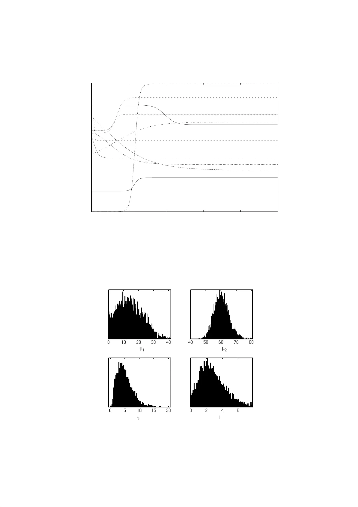
Getting Y our Ey e In: A Ba y esian Analysis of Earl y Dismissals in Cric k et Brendon James Brew er Sc ho ol of Mathematics a nd Statistics The Univ ersit y of New South W ales brendon.bre wer@unsw.edu.au No v em b er 15, 2018 Abstract A Bay esian Surviv al Analysis metho d is motiv ated a nd developed for analysing sequences of scores made by a batsman in test or firs t c la ss crick et. In particular, we exp ect the pres ence of an effect wher eby the distribution of sc o res has mor e probability near zer o than a g eometric distribution, d ue t o the fact that batting is more difficult when the batsman is new at the crea se. A Metrop o lis-Hastings alg o rithm is found to b e efficient at es tima ting the pr op osed parameter s, allowing us to quan tify exactly how la r ge this early - innings effect is, a nd how long a batsman nee ds to b e at the crease in o rder to “g et their eye in”. Applying this mo del to several mo der n play ers shows tha t a batsma n is typically only playing at ab out half of their po tent ial ability when they first ar rive at the cre a se, and gets their eye in surpr isingly quickly . Additionally , some players ar e more “ robust” (hav e a smaller early-innings effect) than o thers, which may hav e implications fo r selection p o lic y . 1 In tro duc tion It is well k nown to crick eters of all skill levels that the lo ng er a batsman is in fo r, the ea sier batting tends to be c ome. This is probably due to a lar g e num b er of psychological and technique-related effects: for example, it is ge ne r ally ag reed tha t it takes a while for a ba tsman’s fo o tw ork to “warm up” and for them to adapt to the subtleties of the pre v ailing conditions and the b owling a ttack. Consequently , it is frequently observed that pla yers are far more likely to b e dis missed ear ly in their innings than is predicted by a c onstant-hazard model, where the pr obability o f g etting out o n your current scor e (called the Hazar d ) is exactly the s ame regar dles s of your c ur rent score . Note that a co nstant ha zard mo del leads to an ex p o nential pr obability distribution ov er the no n-negative int ege r s (i.e. the geo metric distribution) a s describing our pre dictio n of a ba tsman’s scor e. The aim of this pap er is to develop a Bay esian metho d (O’Hagan & F orster, 2004) for inferr ing how a player’s Hazard v aries throughout an inning s , th us giving quantitative answ er s to the questions “how long do we hav e to wait until ba tsmen get their eye in, and how m uch b etter do they really b ecome?” . This question ha s b een addressed previo usly using nonparametric frequentist surviv al analys is (Kim b er a nd Hansford, 1993; Cai, Hyndman and W and, 2 002). Howev er, using a nonpara metric approach in a Bay esian setting would give the hazard function fa r to o muc h freedom a nd would lead to very p o orly constr ained inferences of the haza r d function if applied to individual players. T o simplify matters, this pap er uses a parametric mo del, which is effectively a single change-p oint model with a smo o th transition rather than a sudden jump. 1 2 Sampling Distribution Consider predicting the scor e X ∈ { 0 , 1 , 2 , 3 , ... } that a batsman w ill ma ke in a single innings . W e will now as sign a probability distribution for X , conditional on some parameters . Define a hazard function H ( x ) ∈ [0 , 1] as the probability of b eing dismissed on score x (i.e. P ( X = x )) given that the ba tsman is curr ently o n sc ore x (i.e. given X ≥ x ): H ( x ) = P ( X = x | X ≥ x ) = P ( X = x, X ≥ x ) P ( X ≥ x ) = P ( X = x ) P ( X ≥ x ) (1) Define a backw ar ds cumulativ e distr ibutio n function by: G ( x ) = P ( X ≥ x ) (2) Using G ( x ) ra ther than the conv entional cum ulative distribution F ( x ) = P ( X ≤ x ) simplifies some expres s ions in this case , and a ls o helps b ecause G ( x ) will also ser ve as the likelihoo d function for the “no t-outs”, or uncompleted innings. With this definition, Equatio n 1 b ecomes , after some rearr angement, a difference equation for G : G ( x + 1) = [1 − H ( x )] G ( x ) (3) With the initia l condition G (0) = 1 , this can b e solved, giving: G ( x ) = x − 1 Y a =0 [1 − H ( a )] (4) This is the pro duct of the pr obabilities o f surviving to s core 1 run, times the proba bility of rea ching a sco re of 2 runs g iven that you sco red 1, etc, up to the pr obability of s urviving to scor e x g iven that you score d x − 1 . Thus, the pro bability distribution for X is given by the probability of surviving up to a scor e x and then b eing dismisse d: P ( X = x ) = H ( x ) x − 1 Y a =0 [1 − H ( a )] (5) This is all conditional on a choice o f the hazard function H , which we will par ameterise by pa- rameters θ . Assuming indepe ndence (this is not a physical assertio n, r ather, an ackno wledgement that we ar e not in tere s ted in a ny time dep endent effects for now), the probability distribution for a set of scor es { x i } I − N i =1 ( I and N are the num ber of inning s and not-outs resp ectively) and a set of not-out sc o res { y i } N i =1 is: p ( x , y | θ ) = I − N Y i =1 H ( x i ; θ ) x i − 1 Y a =0 [1 − H ( a ; θ )] ! × N Y i =1 y i − 1 Y a =0 [1 − H ( a ; θ )] ! (6) When the data { x , y } ar e fix e d and known, Equation 6 gives the likeliho o d for any propo sed mode l of the Haz a rd function - that is, for any v alue of θ . The log likeliho o d is : log p ( x , y | θ ) = I − N X i =1 log H ( x i ; θ ) + I − N X i =1 x i − 1 X a =0 log [1 − H ( a ; θ )] + N X i =1 y i − 1 X a =0 log [1 − H ( a ; θ )] (7) 3 P arameterisat ion of the Hazard F unction Rather than s eek clever parameteris ations of H ( x ; θ ) and prior s ov er θ that ar e conjuga te to the likelihoo d, we will ta ke the simpler approa ch of simply defining a mo del and prio r, and doing the inference with a Metrop olis- Hastings sa mpler (C++ source co de and data files for ca rrying this out will b e pr ovided by the author on request). T o capture the phenomenon of “getting your eye in”, the Haza r d function will need to b e high for low x and decrease to a constant v alue as x increases and the batsman b ecomes mor e comfortable. Note that if H ( x ) = h , a cons tant v alue, 2 the sampling distribution b ecomes a geometric distribution with exp ectation µ = 1 /h − 1. This suggests modelling the Hazard function in terms o f a n “ effective batting av er a ge” that v aries with time, which is helpful b ecause it is easier to think o f playing a bilit y in terms of batting av era ges than dis missal pr obabilities. H ( x ) is obtained from µ ( x ) a s follows: H ( x ) = 1 µ ( x ) + 1 (8) A simple change-p oint mo del for µ ( x ) would b e to hav e µ ( x ) = µ 1 + ( µ 2 − µ 1 )Heaviside ( x − τ ), where τ is the change-p oint. How ever, a mor e realistic mo del would hav e µ changing smo othly from one v alue to the other. Replacing the Heaviside step function with a logistic sigmoid function of the for m 1 / (1 + e − t ) g ives the following mo del, which will b e adopted thr o ughout this pa p er : µ ( x ) = µ 1 + µ 2 − µ 1 1 + exp ( − ( x − τ ) /L ) (9) Hence H ( x ) =  1 + µ 1 + µ 2 − µ 1 1 + exp ( − ( x − τ ) /L )  − 1 (10) This has four parameters: µ 1 and µ 2 , the tw o effective abilities of the play er, τ , the midp oint of the tr a nsition b etw een them, a nd L , which descr ib es how abrupt the transition is. As L → 0 this mo del r esembles the simpler change-p oint mo del. A few examples of the kind of hazar d mo dels that can b e describ ed by v a rying these par ameters are shown in Figure 1. It is p oss ible (although we don’t really exp ect it) for the risk of b eing dismissed to incr e ase a s your sc o re incr eases; more commonly it will decrease. Slow or abr upt transitions ar e p o ssible and cor resp ond to different v a lues of L . 4 Prior Distribution Now we must assign a prior pr o bability distribution of the space o f p ossible v a lue s for the parame- ters ( µ 1 , µ 2 , τ , L ). All o f these par ameters a re non-negative and c a n ta ke any p ositive real v alue. It is p ossible to take into a ccount prior correlatio ns b etw een µ 1 and µ 2 (describing the exp ection tha t a player who is excellent when set is a lso more likely to b e g o o d just after arriv ing at the creas e, and that µ 2 is probably greater than µ 1 ). Howev er, this will a lmost certainly be supp or ted by the data anywa y . Hence, for simplicity we assigned the mor e conse r v a tive indep endent Normal(30 , 20 2 ) priors 1 , tr uncated to disa llow neg ative v alues: p ( µ 1 , µ 2 ) ∝ exp " − 1 2  µ 1 − 30 20  2 − 1 2  µ 2 − 30 20  2 # µ 1 , µ 2 > 0 (11) The joint prior fo r L a nd τ is chosen to b e indep endent o f the µ ’s and also indep endent of each other. A typical play er can exp ect to b eco me accusto med to the batting co nditions a fter ∼ 20 runs. An exp onential prior for τ with mean 20 and an exp onential prio r with mean 3 to L were found to pr o duce a rang e of plausible ha zard functions: p ( τ , L ) ∝ exp  − τ 20 − L 3  τ , L > 0 (12) Some hazar d functions sampled fro m the pr ior are displayed in Figure 1. The po sterior distr ibutio n for µ 1 , µ 2 , τ a nd L is prop ortio nal to prior × l ikeli hood , i.e. the pr o duct o f the right ha nd sides of Equations 6, 11 and 12. Qualitatively , the effect of Bay es’ theorem is to take the set of p ossible hazard functions a nd their probabilities (Figure 1) a nd reweigh t the proba bilities a ccording to how well each ha zard function fits the obs e r ved da ta. 1 A reasonable first-order description of the range of exp ected v ariation in batting abilities and h ence our state of knowl edge ab ou t a play er whose identity is unsp ecified - w e intend the algorithm to apply to any pla yer. It is p ossible to parameterise this prior with unk n ow n hyperparameters and infer them from the career data of many pla yers, yielding information about the cric ket population as a whole. How ever, such a calculation is beyond the scop e of this pap er. 3 5 The Data Data were obtained fro m the StatsGuru utility on the Cricinfo website ( http ://ww w.cri cinfo.com/ ) for the following pla yers: Brian La ra, Chris Ca irns, Nasser Hussain, Ga ry Kirs ten, Justin Lang e r, Shaun Pollock, Steve W augh and Shane W arne. These play ers were chosen arbitr a rily but sub- ject to the co ndition o f having re c e nt ly completed long caree r s. A selection of batsmen, q uality all-rounder s and b owlers w as chosen. The MCMC was run for a large num b er of steps - mixing is quite rapid b e c ause the likelihoo d ev a luation is fast and the parameter space is o nly 4-dimensional. F o r brevity , we will display po s terior distr ibutions for Brian L a ra only . F or the other play ers, s um- maries such as the p osterio r means and standard devia tions will b e displayed instead. 6 Results 6.1 Marginal P osterior Distributions In this section we will fo cus on the po sterior distributions of the para meters ( µ 1 , µ 2 , τ , L ) for Brian Lara. The marginal distributions (a pproximated by sa mples from the MCMC sim ulation) ar e plotted in Figure 2. These results imply that when Lara is new to the cr ease, he bats lik e a play er with an average of ∼ 15 , until he has scored ∼ 5 runs. After a transition p erio d with a sc ale length of ∼ 2 runs, (although the form of the logistic functions shows that a tra nsition is more g radual than indicated by L ), he then b egins to bat as though he has an av era ge o f ∼ 60. In this case, the analysis has confirmed the folk lore abo ut Brian L a ra - that if you don’t get him out ear ly , y ou can never really tell when he might get a huge sco r e. “F o rm” do esn’t rea lly come into it. The only sur prise to emerg e from this analys is is the low v alue o f the change-p oint τ - La r a is halfwa y through the pr o cess o f g etting his eye in after scor ing only ab out 5 runs. How ever, there is still a reasona ble a mount of unce r taint y ab out the pa rameters, e ven though Brian Lara ’s lo ng test c a reer consisted of 232 innings. The p osterio r distributio n for Br ian Lar a’s parameters do es not contain strong co rrela tio ns (the maximum absolute v a lue in the correla tio ns matrix is 0 .4 ). This is also true of the p o s terior distributions for the other play ers. Hence, in the next se ction, summaries of the ma r ginal distributions fo r the four parameter s will b e presented for ea ch play er. 6.2 Summaries The es tima tes and uncertainties (p o sterior mean ± s ta ndard devia tion) for the four pa r ameters are presented in T able 1. Figure 3 also shows graphica lly where each of the eight play ers is estimated to lie on the µ 1 - µ 2 plane. One interesting r esult that is ev ident from this a nalysis is tha t it is not just the gritty sp ecialist batsmen that a re r obust in the s e nse that µ 1 is quite high compared to µ 2 . The tw o aggr e ssive allro unders Shaun Pollo ck a nd Chris Cairns also show this trait, and are e ven more robust than, for ex ample, Justin L a nger and Gary Kirsten. It is p o ssible that the techn ique or mindset shown by thes e players is one that do es not r equire muc h warming up, or that it is more difficult to get your eye in at the top of the order than in the middle/low er order - although this o ught to b e a very tent ative conclusion given that it is based on o nly tw o examples. The estimated v a lue of µ 1 for Steve W aug h is low er than a ll other play ers in the sa mple apar t from Shane W a r ne. Even Shaun Pollock app ears to b e a be tter batsman than Steve W augh at the b eginning of his innings. The plausibility o f this s ta tement can b e mea sured by asking the question “what is the p oster ior probability that H P ollo ck (0) < H W aug h (0)?”. F ro m the MCMC output, this pro bability w as found to b e 0 .92. The ma rginal likeliho o d or “evidence” for this entire mo del and choice o f prio rs can be measured effectively using annealed impo rtance sa mpling, or AIS (Neal, 1998; Jar z y nski, 1997a,b). AIS is a very gener ally applicable MCMC-based algor ithm tha t pro duces an unbiased estimate of Z = R prior ( θ ) × likel ihood ( θ ) dθ . Z is the proba bilit y of the data that were a ctually observed, under the mo del, av erage d over all po ssible parameter v a lues (weigh ted according to the prior ). It is the cruc ia l quantit y for up dating a state of knowledge ab out which of tw o distinct mo dels is correct (MacKay, 2003; O’Hag an & F or ster, 200 4). T o test our mo del for the hazard function, we computed the ev idence v alue for each play er for the v arying- hazard model and a lso for a constant hazard mo del, with a tr unca ted N (30 , 20 2 ) prior on the cons ta nt effective average. The log a rithm 4 T able 1: P arameter estimates for the play ers studied in this pap er . The righ t hand column, the logarithm of the Ba y es F actor, s ho ws that the d ata su pp ort the v arying hazard mo del ov er a constant hazard m o del by a large factor in all cases. T h e smallest Bay es F actor is still o v er 250 0 to 1 in fa vour of the v arying Hazard Model. Th us, the v arying hazard m o del w ould lik ely still b e significantl y fav our ed ev en if the priors for the parameters w ere slightl y m o dified. Pla y er µ 1 µ 2 τ L log e ( Z ) log e ( Z/ Z 0 ) Cairns 26.9 ± 9.2 36.7 ± 5.5 14.5 ± 17.7 3.1 ± 3.0 -444.11 8.82 Hussain 15 .6 ± 9.1 42.1 ± 4.4 5.2 ± 7.1 2.2 ± 1.0 -707.1 6 12.28 Kirsten 16.6 ± 9.3 54.1 ± 5.7 7.3 ± 5.5 2.9 ± 2.4 -757.1 6 16.94 Langer 24.3 ± 11.5 49.6 ± 4.9 8.9 ± 14.3 2.8 ± 2.9 -810.3 4 11.66 Lara 14.5 ± 8.3 60.2 ± 4.7 5.1 ± 2.9 2.8 ± 1.8 -1105 .65 21.62 P ollo c k 22.1 ± 7.7 38.9 ± 5.4 9 .7 ± 9.3 3.1 ± 2.9 -519.3 9 7.87 W arne 3.5 ± 2.0 21.1 ± 2.0 1.1 ± 0.6 0.5 ± 0.4 -686.5 9 22.54 W augh 10.5 ± 5.5 57.3 ± 4.4 1.8 ± 1.6 0.8 ± 1.2 -1030 .69 25.29 Prior 32.8 ± 17.6 32. 8 ± 17.6 20.0 ± 20.0 3.0 ± 3.0 N/ A N/A of the Bayes F actor (evidence r atio) describing how well the da ta suppo rt the v arying - hazard mo del ov er cons tant hazar d is shown in the right-hand column of T able 1. Since these were computed using a Monte-Carlo pro cedure, they are not exact, but the AIS sim ulatio ns w ere run for long enough so that the s tandard error in the Bayes F actor for each player was less than 5 % of its v alue. The data decisively fav our the v arying-ha zard mo del in all cases, and this would b e exp ected to per sist under s light c hanges to the ha zard function para meterisation o r the prior distributions. 6.3 Predictiv e Hazard F unction In the usual wa y (O’Hagan & F or ster, 2 004), a predictive distribution for the next data p oint (score in the next innings) can be found by averaging the sa mpling distribution (Eq uation 6) ov er all p oss ible v a lues of the parameter s that are a llow ed by the p os terior. Of course , all of these play ers hav e re tir ed, so this pr ediction is simply a conceptual device to ge t a single distribution ov er scor es, and hence a single estimated haza rd function via Equatio n 1. This predictive haza rd function is plotted (in terms of the effective average) for three play ers (Brian Lara , Justin Langer and Steve W augh) in Figure 4. The latter tw o are noted for their grit, whilst B rian Lara is c o nsidered an agg ressive batsman. These different styles may translate to noticable differences in their predictive hazar d functions. It is clear from Fig ure 4 that Justin Langer is mor e “ro bust” than Bria n La ra, a s the difference b etw een his abilities when fres h and when set is smaller ( P   µ 2 µ 1  Lar a >  µ 2 µ 1  Lang er  = 0 . 8 0). This is proba bly a go o d trait for an op ening batsman. On the other hand, Steve W aug h is actually significa ntly worse when he is new to the crea se than Brian Lara ( P ( H W aug h (0) > H Lar a (0)) = 0 . 85 ). This surprising result shows that po pular p erceptions are not necess a rily a ccurate, given that many p eople re g ard Steve W augh as the play er they would choo se to play “for their life” 2 . How ever, Steve W a ugh’s pre dic tive hazar d function has a tr a nsition to its high equilibr ium v a lue that is so oner a nd faster than b o th Lara and Langer ( P ( τ W aug h < τ Lang er and τ W aug h < τ Lar a and L W aug h < L Lang er and L W aug h < L Lar a ) = 0 . 53, the prior pro bability of this is 0.06 25). Therefo r e, p er ha ps his reputation is upheld, except at the very b eginning of an inning s. Note that the ge neral tendency of the effective av erag e to drift upw ards as a function of score do es not imply that all batsman get b etter the longer their inning s go es on - since o nce the transitio n has o ccurred, our mo del says that the ha zard r ate sho uld stay bas ic ally consta nt . Instead, the hazard function of the predictive distribution describ es a gra dual change in our state of knowledge: 2 T ec hn ically , the correct choice w ould b e to choose a p la yer that minimised the exp ected loss, where loss is defi ned as the amount of injury inflicted on the sp ectator as a function of th e batsman’s score. 5 the longer a batsman stays in, the more convinced we a re tha t our estimate of their ov erall ability µ 2 should b e highe r than our prior estimate. This is why there is a n upw ar ds tendency in the predictive a bility function for all play ers , even w ell after the change-p o int transition is co mpleted. 7 Conclusions This paper has presented a simple mo del for the hazard function of a batsman in test or fir st class crick et. Applying the mo de l to data from several crick eters , we fo und the exp ected conclusio n: that batsmen are mor e vulner able towards the b eginning o f the innings. Ho wev er, this ana ly sis now provides a quantitativ e measur e ment o f this effect, showing how significant it is, and the fact that ther e is substantial v a riation in the size of the effect for different crick eters . Surpris ingly , we found that Steve W augh was the second most vulnerable player in the sa mple at the beg inning o f an innings - only Shane W arne, a b owler, w as was more vulnerable. Even Sha un Pollo ck is b etter at the b eg inning of his innings. This surprising r esult would hav e be e n very hard to anticipate. F r om this star ting p oint, ther e are s everal p ossible av enues for further rese a rch. One int ere sting study would inv olve muc h larger samples o f play ers s o we can identify a ny trends. F or instance, is it true that all-ro under s are more robust batsman in general, or are Chris Cairns and Shaun Pollock atypical? Also, it should b e p ossible to cr eate a more rig orous definition of the notio n of robustness discussed ab ov e. Once this is done , we could characterise the p opula tion as a whole, and search for pos sible corr elations b etw een batting av er age, strike-rate (runs scored per 100 balls faced) and robustness. Mo delling the entire cr ick et p opulation w ould also allow for a more ob jective choice for the par ameterisa tion of the haza rd function, a nd the prior distribution ov er its para meter space. Depending on the results, these kinds of analys es could have implications for selection p olicy , esp ecially for o pe ning batsmen where consistency is a highly des ir able tr ait. References Cai, T., Hyndman, R.J. a nd W and, M.P . (20 02). Mixe d mo del-b ase d hazar d estimation , Jour nal of Computational and Gra phical Statistics, 1 1, 7 8 4-79 8. Jarzynsk i, C. 19 97a, Equilibrium fr e e-ener gy differ enc es fr om none quilibrium me asur ements: A master-e quation appr o ach , Physical Review E, 5 6 , 5018 . Jarzynsk i, C. 19 97b, None quilibrium Equality for F r e e Ener gy Differ enc es , Physical Review Letters, 78, 2 690. Kimber, A. C., Hansfo r d, A. R., A Statistic al Anaylsis of Batting in Cricket , Jour nal of the Ro yal Statistical So ciety . Ser ies A (Statistics in So ciety), V o l. 156, No. 3. (1993 ), pp. 4 43-4 5 5. MacKay , D. J. C. 2003 , Information The ory, In fer en c e and L e arning Al gorithms , ISBN 05216 4298 1. Cambridge, UK: Cambridge Univ ersity Pre s s. Neal, R. M. 1998 , Anne ale d Imp ortanc e Sampling , ar Xiv:physics/980300 8 , T echnical Re- po rt No. 9 805 (revised), Dept. of Statistics, Univ ersity o f T oronto. Av ailable online at http:/ /www. cs.toro nto.edu/~radford/papers-online.html O’Hagan, A., & F or s ter, J. 2004 , Kendal l’s advanc e d t he ory of statistics. V ol.2B: Bayesian infer- enc e , 2nd ed., by A. O’Hag an and J. F or ster. 3 volumes. London: Hodder Arnold, 20 04. 6 10 20 30 40 50 0 20 40 60 80 100 Effective Average Score (x) Figure 1: Illus trativ e examples of the kind of functions pro duced by Equation 9, with a range of t ypical v alues (c hosen from the prior, see Section 4) of th e four p arameters µ 1 , µ 2 , τ and L . Figure 2: Results for the f our parameters for Brian Lara. The top tw o panels sho w th e p osterior distributions for his t wo abilities (effectiv e batting a verag es) µ 1 and µ 2 , while the low er panels sh o w the d istributions for the c hange-p oint τ and change -timescale L . See the text for in terpretation. 7 Figure 3: Estimated lo cation of eac h of the pla ye rs on the µ 1 - µ 2 plane. T he line corresp onds to µ 2 = µ 1 , and the closer a play er is to the line, the more robust the pla yer. Surp risingly , Shau n P ollo c k and Chr is Cairns lie closest to the line. Although eac h pla y er has b een rep r esen ted by a p oint on th is p lot, th ese are only estimates (p osterior means), and eac h p oin t is actually just the centre of a large zone of u ncertain t y . 0 10 20 30 40 50 60 0 10 20 30 40 50 60 µ 2 µ 1 Posterior Mean µ 2 = µ 1 Warne Cairns Pollock Hussain Lara Waugh Kirsten Langer Figure 4: Predictive Hazard F unctions for Brian Lara, Justin Langer and Steve W augh. As exp ected, Justin Langer prov es to b e less vu ln erable th an Brian Lara at th e b eginn in g of his in n ings. Ho w ev er, surpr isingly , Stev e W augh is more vulner ab le than Brian Lara, although he gets his ey e in so oner. 8 0 10 20 30 40 50 60 0 10 20 30 40 50 60 µ 2 µ 1 Posterior Mean µ 2 = µ 1