Small Approximate Pareto Sets for Bi-objective Shortest Paths and Other Problems

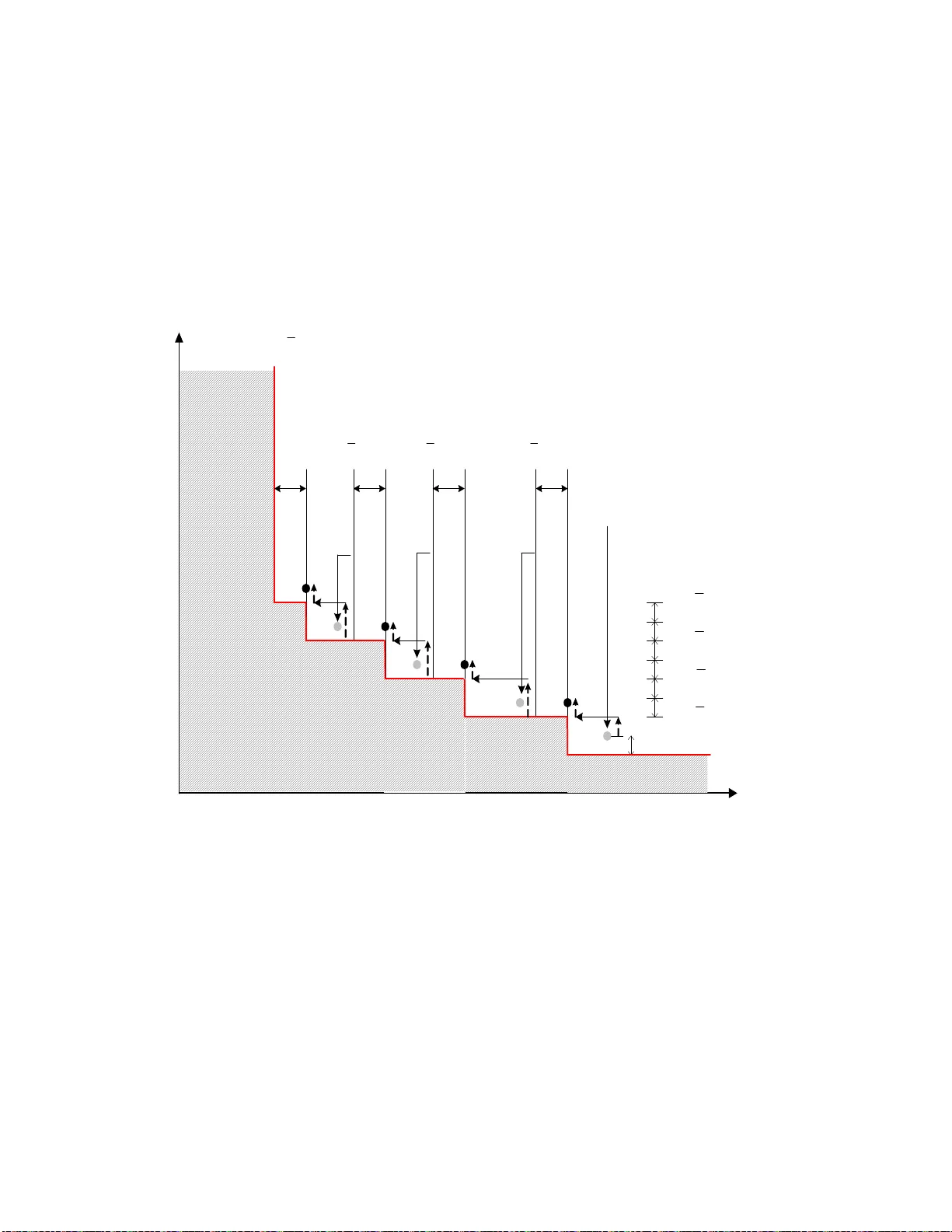
Small Approxi mate P areto Sets for Bi-objecti ve Shortest Paths and Other Problems ∗ Ilias Diakonikolas † ilias@cs.c olumbia.e du Mihalis Y annakakis ‡ mihalis@cs .columbia .edu Abstract W e in vestigate the problem of computin g a minimu m set o f solutions that approxima tes within a speciﬁed accuracy ǫ the Pareto curve of a multiobjective optimization problem. W e show th at for a broad class o f bi-o bjective pro blems (contain ing many important widely studied pr oblems such as shortest paths, spanning tree, and many others), we can compute in polyno mial time an ǫ -Pareto set that contains at most twice as many solu tions as the minimum such set. Furthermor e we show th at the factor of 2 is tight for these problem s, i.e., it is NP-hard to d o better . W e present upp er and lower bou nds for three o r more objectives , as well as for th e dual p roblem of com puting a speciﬁed numbe r k of so lutions which provide a good approxima tion to the P areto cu rve. ∗ A preliminary version of this work appeared in the Proceedings of the 10th International W orksh op on Approximation Al go- rithms for Combinatorial Optimization Problems ( APPRO X’ 0 7 ), 2007, pp. 74–88. † Supported by NSF grant CCF-04-30946, NSF grant CCF-07-28736 and an Alexand er S. Onassis Foundation Fello wship. ‡ Supported by NSF grant CCF-04-30946 and NSF grant CCF-07-28736. 1 Introd uction In many decision making situatio ns it is typically the case that more than one criteria come into play . For exa mple, when purch asing a product (car , tv , etc.) we care about its cost , qualit y , etc. When choosing a rou te we may care about the time it tak es, the distance tra velled , etc. When desi gning a net work w e may care about its cost, its capac ity (the load it can carry), its cover age. This type of multicriteria or multiobjectiv e proble ms arise acros s many div erse discipli nes, in engineer ing, in economics and b usiness, healthc are, and others . The area of multiobje ctiv e optimization has been (and continu es to be) extensi vely in vestigate d in the management science and optimization communiti es with m any papers , conferenc es and books (see e.g. [Cli, Ehr, EG, FGE, Mit]). In multiobjec tiv e proble ms there is typi cally no uniformly best solution in all objecti ves , but rather a trade-o ff between the diff erent objecti ves. This is captured by the trade-of f or P ar eto curve , the set of all soluti ons whose vector of objecti ve value s is not dominated by any other solution. The trade-o ff curve repres ents the range of reasonabl e “optimal ” choices in the design space; they are precisely the op timal soluti ons for all possible global “utility” functions that depend mono tonically on the dif ferent objecti ves . A decisi on maker , presented w ith the trade-of f curve, can select a solution that correspond s best to his/her prefere nces; of c ourse differe nt users generall y may ha ve diff erent pre ferences an d sele ct dif ferent solu tions. The problem is that the trade-of f curv e has typic ally expone ntial s ize (for discrete proble ms) or is inﬁnite (for continuo us problems), and hence w e cannot constru ct the full curve. Thus, we ha ve to contend with an approx imation of the curve: W e want to compute efﬁcien tly and present to the decisio n mak ers a small set of solutions (as small as possi ble) that repre sents as well as possible the whole range of choice s, i.e. t hat pro vides a good approxi mation to the Pareto curve. Indeed this is the und erlying goal in much of the re- search in th e multiobjecti ve area, with man y heur istics proposed, usually ho wev er without any p erformance guaran tees or complexi ty analysis as we do in theoreti cal computer science. In recent years we initiated a systematic in vestiga tion [P Y1, VY] to de velop the theory of multiob- jecti ve appro ximation along similar rigorous lines as the approximation of single objecti ve probl ems. The approx imation to the Pareto curv e is cap tured by the concept of an ǫ -P ar eto set , a set P ǫ of solutions that approx imately dominates ev ery other solution; that is, for ev ery solution s , the set P ǫ contai ns a solution s ′ that is within a factor 1 + ǫ of s , or be tter , in all the ob jecti ves. (As usual in approximati on, it is assumed th at all objecti ve functions take positiv e v alues.) Such an approx imation was studied before for certa in proble ms, e.g. multiobjecti ve shortest paths, for which Hansen [Han] and W arb urton [W a] sho wed ho w to construct an ǫ -Pareto set in polyno mial time (for ﬁxe d n umber of objecti ves). Note that typically in most real-life multiobj ectiv e prob lems the number of objec tiv es is small. In fact, the great majority of the multiobject iv e literat ure concer ns the case of two ob jecti ves. Consider a multiobject iv e pr oblem with d objecti ves , for example shortest path with cost and time object iv es. For a giv en instance, and error tolerance ǫ , we would like to compute a smallest set of solutions that form an ǫ -Pareto set. Can we do it in polynomial time? If not, how well can we approxi mate the smallest ǫ -Pareto set? Not e that an ǫ -Pareto set is not unique: in genera l the re are man y such sets , some of which can be v ery small and some v ery lar ge. First, to hav e an y hope we must ensure that there ex ists at least a polyn omial siz e ǫ -Pareto set. Indeed , in [PY1] it was sho wn that this is the case for ev ery multiobj ectiv e proble m with a ﬁxed number of polynomially computa ble objecti ves . S econd we must be able to construct at least one such set in polynomia l time. This is not alw ays possibl e. A necessary and suf ﬁcient conditio n for po lynomial computab ility for all ǫ > 0 is th e exist ence of a p olynomial algorit hm for the follo wing Gap pr oblem : Giv en a vector of valu es b , either compute a soluti on that dominates b , or determine that no soluti on dominates b by at least a fact or 1 + ǫ (in all the objecti ves). Man y multiobjecti ve problems were sho wn to hav e such a routine for the G ap prob lem (and man y others hav e been shown subseq uently). Construc tion of a polyno mial-size approxi mate Pareto set is useful, but not good enough in itself: For exa mple, if w e plan a trip, we want to exa mine just a few possible routes, not a polynomial number in the 1 size of the m ap. More generally , in typical multicrit eria situatio ns, the selected representat iv e solutio ns are in vestiga ted more thoroughl y by the de cision mak er (designer , physicia n, corporatio n, etc.) to assess the dif ferent cho ices and pick the most preferable one, based pos sibly on ad ditional fact ors that are perhaps not formalize d or not e ven quant iﬁable. W e thu s wa nt to select as small a set as possibl e that achie ves a desire d ap proximation . In [VY] the problem of constructin g a minimum ǫ -Pareto set was raised formally and in vest igated in a gener al framewo rk. It was shown tha t for all bi-ob jecti ve problems w ith a p olynomial- time Gap routine, one can con struct an ǫ -Pareto set tha t contains at most 3 times the numbe r of points of th e smallest s uch set; furthermo re, the facto r 3 is best p ossible in the sense that fo r some probl ems it is NP-hard to do better . Further results were sh own f or 3 and more o bjecti ves, and fo r oth er related que stions. Note that althou gh the f actor 3 of [VY] is best possible in general for two object iv es, one may be able to do better for speciﬁc prob lems. W e sho w in this paper , that for an importan t class of bi-object iv e problems (c ontaining man y widely studie d na tural ones such as shor test pa ths, spa nning tree, k napsack, sche duling problems and others) we can ob tain a 2 -ap proximation , an d further more the fa ctor of 2 is tight for them, i.e., it is N P-hard to do better . Our algorithm is a genera l algori thm that relies on a routine for a strong er version of the Gap proble m, namely a routine that solv es approx imately the follo wing Restricte d pr oblem : G i ven a (hard) bound b 1 for o ne objecti ve, comput e a solutio n that optimizes appro ximately the seco nd objecti ve subjec t to the bound . Many prob lems (e.g. shortest paths, etc.) hav e a polynomial time approximati on scheme for the Restricte d problem. For a ll suc h proble ms, a 2 -a pproximatio n to the minimum ǫ -Pareto set can be comput ed in po lynomial time. Furthermore, the number of c alls to the R estricte d routine (an d an as sociated equi va lent dual routin e) is linear in the size OPT ǫ of the optimal ǫ -Pareto set. The bi-obje ctiv e shortes t path probl em is probably the most well-studie d multiobjecti ve problem. It is the paradig matic problem for dynamic programming (th us can e xpress a v ariety of problems), and arise s itself direc tly in many con texts. One area i s network routi ng with vari ous QoS criteria (see e.g. [CX 2, ESZ, GR+, VV]). For example , an interesting p roposal in a recent pap er by V an Miegh en an d V anden berg he [VV ] is to ha ve the netwo rk operator adv ertise a portfolio of offer ed QoS solutio ns for their network (a trade-of f curv e), and the n users can sel ect the so lutions that bes t ﬁt their ap plications . Ob viously , the p ortfolio cannot includ e ev ery sin gle possibl e route, and it would mak e sense to select carefu lly an “optimal ” set of solut ions that cov er well the whole rang e. Other application s include th e tr ansportati on of haz ardous materia ls (to minimize risk o f accident, and populati on exposur e) [EV], and man y others; we refer to the ref erences, e.g. [EG ] contain s po inters to the extensi ve literatur e on shortest path s, spanning trees, knapsack, and the other problems. Our algorithm app lies not only to th e abo ve standard combinatorial prob lems, but more genera lly to any bi-objecti ve problem for which we hav e av ailabl e a routine for the Restricted problem; the object iv e functio ns and the routine itself could be complex piece s of softwa re witho ut a simple mathematica l exp ression. After giv ing th e b asic deﬁnitio ns and backg round in Section 2, we pre sent in Sectio n 3 our general lower and upp er bound result s for bi-objec tiv e problems, as well as a pplication s to speciﬁc probl ems. In Section 4 we present some results for d = 3 and more objecti ves . Here w e assu me only a Gap routin e; i.e. these resul ts apply to all pr oblems with a polyn omial time con structible ǫ -Pareto set. It w as sh own in [VY] that for d = 3 it is in general impossib le to get a constant facto r approxi mation to the optimal ǫ -Pareto set, b ut one has to relax ǫ . Combining results from [VY] and [KP] w e show that for any ǫ ′ > ǫ w e can constru ct an ǫ ′ -Paret o set of size c OPT ǫ , i.e. within a (lar ge) cons tant factor c of the size OPT ǫ of the optimal ǫ -Pareto set. For genera l d , the prob lem can be red uced to a Set Co ver p roblem whose VC dimens ion and codimens ion are at most d , and we can constr uct an ǫ ′ -Paret o set of size O ( d log OPT ǫ )OPT ǫ . W e discuss also the D ual problem: For a speciﬁed number k of points, ﬁnd k points that pro vide the best appro ximation to the Pareto curv e, i.e. that form an ǫ -Pareto set with the minimum possible ǫ . In [VY] it was sh own that for d = 2 objecti ves the problem is NP-hard, but we ca n approximat e arbitrari ly well (i.e. there is a PT AS) t he minimum appr oximation ratio ρ ∗ = 1 + ǫ ∗ . A s we’ ll see, for d = 3 this is n ot possible , 2 in fact one cannot get any multiplica tiv e approximatio n (unle ss P =NP). W e use a relationsh ip of the Dual proble m to the asymmetric k -cente r probl em and techni ques from the latter problem to sho w that the D ual proble m can be approximate d (for d = 3 ) within a consta nt power , i.e. we can compute k points that cover e very point on the Pa reto curve within a f actor ρ ′ = ( ρ ∗ ) c or bette r in all ob jecti ves, for some consta nt c . (It follo ws from our results that c ≤ 9 .) For small ρ ∗ , i.e. when there is a set of k points that provid es a good approx imation to the Pareto curve, constan t facto r and constant po wer are related, b ut in general of course the y are not. 2 Deﬁnitions and Backgroun d A multiobj ectiv e optimizatio n problem Π has a set I Π of val id instan ces , ev ery instance I ∈ I Π has a set of solutio ns S ( I ) . There are d ob jecti ve functi ons, f 1 , . . . , f d , each of which maps e ver y instanc e I and solu tion s ∈ S ( I ) to a val ue f j ( I , s ) . The p roblem speciﬁes for each o bjecti ve whether it is to be maximized or minimized. W e assume as usual in approximatio n th at the objecti ve functions ha ve positi ve ration al v alues, and that they are polynomial-ti me computable. W e use m to denote the m aximum number of bits in numerato r and denominator of the objecti ve function val ues. W e say that a d -vect or u dominates anoth er d -v ector v if it is at least as good in all the objecti ve s, i.e. u j ≥ v j if f j is to be maximize d ( u j ≤ v j if f j is to be minimized ). Similarly , we de ﬁne dominatio n between any solution s accordin g to the d -v ectors of their objecti ve v alues. Giv en an instance I , the P ar eto set P ( I ) is the set of undomin ated d -v ectors of values of the solutions in S ( I ) . Note that for any instance, the Pareto set is uniqu e. (As usual we are also interested in solution s that realize these v alues, but w e will often blur the dist inction and refer to the Pareto set also as a set of solutions that ach iev e these v alues. If there is more than one undomina ted soluti on with the same objecti ve val ues, P ( I ) contains one of them.) W e say t hat a d -vec tor u c -co vers another d -vecto r v if u is at lea st as good as v up to a facto r of c in all the objecti ves, i.e. u j ≥ v j /c if f j is to be maximized ( u j ≤ cv j if f j is to be minimized). G iv en an insta nce I an d ǫ > 0 , an ǫ -P ar eto set P ǫ ( I ) is a set of d -vector s of val ues of solut ions that (1 + ǫ ) -co ver all vectors in P ( I ) . For a gi ven inst ance, there may exist man y ǫ -Pareto s ets, and the y may ha ve ver y diff erent sizes. It is sho wn in [PY1] tha t for e very multio bjecti ve optimizatio n problem in the af orementione d frame work, for e very instan ce I and ǫ > 0 , there exist s an ǫ -Pareto set of size O ((4 m/ǫ ) d − 1 ) , i.e. polynomial for ﬁxed d . An approximate Pareto set al ways exists, but it may not be cons tructible in poly nomial time. W e say that a multiobjecti ve problem Π has a polynomia l time approximation scheme (respecti ve ly a fully polynomial time approximatio n scheme) if there is an algorithm, which, giv en instan ce I and a rational number ǫ > 0 , constr ucts an ǫ -Pareto set P ǫ ( I ) in time polynomial in the size | I | of the ins tance I (respec tiv ely , in time polyn omial in | I | , th e representa tion size | ǫ | of ǫ , and in 1 /ǫ ). Let MPT AS (resp. MFPT AS) denot e the clas s of multiob jecti ve problems that hav e a polynomial time (respe ctiv ely fully polyn omial time) approximatio n scheme. There is a simple necessary and sufﬁcien t co ndition [P Y1], which relates the efﬁcient comput ability of an ǫ -Pareto set for a multi-objec tiv e pro blem Π to the follo wing GAP Pr oblem : giv en an instance I of Π , a (positi ve rational) d -vector b , and a rational δ > 0 , eith er return a solution whose vecto r dominates b or report that there does not exist any soluti on whose vector is better than b by at least a (1 + δ ) factor in all of the coordinates . As shown in [PY1], a problem is in MPT AS (resp. MFPT AS) if and only if there is a subroutine GAP that solves the G AP problem for Π in time polyno mial in | I | and | b | (resp. in | I | , | b | , | δ | and 1 /δ ). W e say that an algorithm that uses a routine as a black box to access the solutions of the multiobject iv e proble m is generic , as it is not gea red to a particular p roblem, b ut a pplies to all of th e p roblems fo r which the particu lar routine is av ailabl e. All that such an algorithm needs to kno w about the input instance is bounds on the m inimum and maximum possi ble v alues of the objecti ve functions. (For example, if the object iv e functi ons are positi ve rational numbe rs whose numerator s an d denomina tors h av e at most m bits, then an 3 obv ious lo wer bound on the object iv e v alues is 2 − m and an obviou s upper bound is 2 m ; h owe ver , fo r sp eciﬁc proble ms better bound s may be av ailabl e.) Based on the bounds, the algorithm calls the giv en routin e for certain v alues of its parameters, and uses the returned results to compute an approximate Pareto set. For a gi ven inst ance, t here may ex ist many ǫ -Pareto sets , and they may hav e very dif ferent sizes. W e want to compute one with the smallest possible size, w hich we’ll denote OP T ǫ . [VY] giv es generic algorithms that compute smal l ǫ -Pa reto se ts and are applicab le to all mul tiobjecti ve pr oblems in M(F)PT AS, i.e. all proble ms posses sing a (fully) polyno mial G AP routine . They consider the follo wing “dual” proble ms: Giv en an instance and an ǫ > 0 , construc t an ǫ -Pareto set of as small size as possible . And dual ly , gi ven a bou nd k , compute an ǫ -Paret o set with at most k points that has as small an ǫ v alue as pos sible. In the case of two objecti ves, they giv e an algorithm that compu tes an ǫ -Pareto set of size at most 3OPT ǫ ; they sho w that no algori thm can be better than 3 -approximate in this setting . For the dual problem, they show that the opt imal v alue of the ratio ρ = 1 + ǫ can be approxi mated arbitrari ly closely . For three object iv es, the y sho w that no algorithm can be c -approximate for any constan t c , unl ess it is allo wed to use a larger ǫ v alue. They also gi ve an algorithm that cons tructs an ǫ ′ -Paret o set of cardi nality at most 4OPT ǫ , for an y ǫ ′ > (1 + ǫ ) 2 − 1 . In a gen eral multiobje ctiv e problem we may hav e bot h minimization and maximiza tion objecti ves. In the remainder , we will assume for con venience that all objecti ves a re minimizat ion ob jecti ves; this is without loss of general ity , since we can simply tak e the reciproca ls of maximization objecti ves. Notation : Fo r a positi ve intege r n ∈ N ∗ , we will deno te by [ n ] the set { 1 , 2 , . . . , n } . 3 T wo Objectiv es W e use the follo wing notatio n in this sectio n. Consider the plane whose coordi nates correspond to the two object iv es. Every solution is mapped to a point on this plane. W e use x and y as the two coordin ates of the plane. If p is a point, we use x ( p ) , y ( p ) to denote its coordinat es; that is, p =  x ( p ) , y ( p )  . W e con sider the class of bi-objecti ve problems Π for which we ca n approximately minimize one objec- ti ve (say the y -coordin ate) subject to a “h ard” constra int on the other (the x -coordinate) . Our basic pri mitiv e is a polynomial time (or ful ly polyno mial time) routine for the fo llowing Restric ted pr oblem (for the y - object iv e): Gi ven an insta nce I ∈ I Π , a (positi ve ra tional) bound C and a paramete r δ > 0 , eith er return a so- lution point ˜ s sati sfying x ( ˜ s ) ≤ C and y ( ˜ s ) ≤ (1 + δ ) · min { y ov er all solutions s ∈ S ( I ) havin g x ( s ) ≤ C } or correctl y report that there does not exist any solutio n s such that x ( s ) ≤ C . For simplic ity , we will drop the in stance from th e notat ion and use Res trict δ ( y , x ≤ C ) to denote the solution retu rned by the corre- spond ing routin e. If the routine do es not retur n a solut ion, w e will say that it re turns N O. W e say that a routin e Restrict δ ( y , x ≤ C ) runs in polyno mial time (resp. fully polyn omial time) if it s running time is polyn omial in | I | and | C | (resp. | I | , | C | , | δ | and 1 /δ ). The Restricte d problem for the x -obje ctiv e is d eﬁned analog ously . W e will also use the Restricted routine with strict inequality bounds; it is easy to see that they are polyno mially equiv alent. Note that in ge neral the two objecti ves c ould b e no nlinear and comple tely unrel ated. Mor eove r , it is possib le that a bi-objecti ve problem possesses a (fully) polynomial Restricted routine for the one objecti ve, b ut not for the other . T he consider ed clas s of bi-objecti ve probl ems is quite broad and contains m any well- studie d natural o nes, most notably the bi-object iv e shortest pa th an d span ning tree problems (see Section 3.3 for a more detai led list of appli cations). The structu re of this sect ion is as follows: In Section 3.1, we show that, ev en if the giv en bi-objecti ve proble m possesses a fully polynomial Restricted routine for both obje ctives , no generic algorith m can guar - antee an ap proximation ratio better than 2 . (This lower bound ap plies a fortio ri if the Restr icted rou tine is a vail able for on e objecti ve only .) Furthermor e, we sho w that for two such natural problems, namely , the bi-objecti ve shortest path and spanning tree problems, it is NP -hard to do better than 2 . In Section 3.2 4 we giv e a matchi ng upper bound : w e present an ef ﬁcient 2 -ap proximation algorithm that app lies to all of the problems that possess a polynomial R estrict ed routin e for one of the two object iv es. In S ection 3.3 we discus s some applicatio ns. 3.1 Lower bound T o prov e a lo wer bound for a generic proce dure, we pre sent two Pareto sets which are indis tinguishab le from ea ch other using the Restr icted routine as a black box, yet whose s mallest ǫ -Pareto sets ar e of dif ferent sizes. Pro position 3.1. Conside r the class of bi-object ive pr oblems that possess a fully polyno mial R estricte d r outine for both objectiv es. Then, for a ny ǫ > 0 , ther e is no polyno mial time g eneric algorithm that appr ox- imates the size of the smallest ǫ -P ar eto set P ∗ ǫ to a facto r better than 2 . Pr oof. Fix a rational ǫ > 0 and con sider the follo w ing set of points: p = ( x ( p ) , y ( p )) , q =  x ( p ) 1+2 ǫ 1+ ǫ , y ( p ) 1+ ǫ  , r =  x ( p ) 1+ ǫ , y ( p ) 1+2 ǫ 1+ ǫ  , p q =  x ( p ) + 1 , y ( p )(1 − 1 x ( p ) )  and p r =  x ( p )(1 − 1 y ( p ) ) , y ( p ) + 1  , where x ( p ) , y ( p ) > 1 + 1 ǫ (Figure 1). Let P = { p, q , r , p q , p r } and P ′ = { q, r, p q , p r } be the feasible (solution ) sets corre sponding to two input inst ances. Note that p (1 + ǫ ) -cove rs all the point s, p q does not (1 + ǫ ) -co ver r (due to the x coord inate) and p r does not (1 + ǫ ) -cov er q (due to the y coordina te). It is easy to see that the smalle st ǫ - P areto set f or P consists of only on e point (namely po int p ), while the small est ǫ - Pareto se t for P ′ must include two points . W e can s how that a gen eric algorithm is guar anteed to tell the dif ference between P and P ′ only if 1 /δ is expo nential in the size of the input. The arg ument is very similar to the proof of Theorem 1 in [VY]. L et x ( p ) = y ( p ) = M , where M is an integer val ue exponen tial in the size of the input and 1 /ǫ . By expl oiting the fa ct that, in some cases, our primiti ve is not uni quely deﬁned , we can ar gue that a polynomial time generi c algorith m cannot distingui sh between instances P and P ′ . More speciﬁcally , a generic algorithm is guar anteed to tell the diff erence between P and P ′ only if the tolerance δ is in verse expone ntial in the size of the input . First, note that both point s q and r can be efﬁcien tly comp uted by appropri ately using the giv en rou- tine; these tw o po ints suf ﬁce to (1 + ǫ ) -cov er the feasibl e set in both cases. Distinguishi ng between the two instances means determin ing whether p is part of the solution. Assume that we use the operation Restrict δ ( x, y ≤ C ) , w here C ∈ [ y ( p ) , y ( p r )) . It is easy to see that this is the only “meaningful ” opera tion using th is routin e as a bl ack box. T hen, e ven if p is par t of the s olution, by de ﬁnition, Restrict δ can r eturn p q as long as x ( p q ) ≤ (1 + δ ) x ( p ) or equi vale ntly δ ≥ 1 M . But since w e want a polynomial time algorithm, 1 δ has to be pol ynomial in lg M ; hence, the latter constra int must hold. By symmetry , the same property holds for the R estrict δ ( y , · ) rou tine. Therefore, using each of thes e routi nes as a black box, a polynomial time algori thm cannot determine if p is part of the solution, and it is thus forced to take at least two points, ev en when it is presented with the set P . Note that the abov e conﬁgurat ion can be replicated to show that it is impossib le for a generic algor ithm to determine w hether the smallest ǫ -Pareto set has k points or 2 k points are needed .  In fact, we can prov e someth ing stronger (assumin g P 6 = N P) for the bi-object iv e s hortest path ( BSP ) and spann ing tree ( BST ) probl ems. In the BSP problem, we are gi ven a (directed or undirected ) graph, positi ve ration al “costs” and “delays” for each edge and two speciﬁed nodes s and t . The set of feasible solutions is the set of s − t paths. The ob jecti ves (to be minimize d) are linear , i.e. the “ total weight” of a path equals the sum of the weights of its edges. The B ST problem is deﬁned analogously . These problems are w ell-kno wn to poss ess polyn omial Restricte d routines for both objecti ves [LR, GR]. W e show the foll owing: 5 x y p q r p q p r Figure 1: A polynomial time generic algorith m cannot determine if p is a solu tion of the giv en instance. Theor em 3.2. a. F or the BSP pr oblem, for any k fr om k = 1 to a polynomial, it is NP-har d to disting uish the case that the minimum size OPT ǫ of the optimal ǫ -P ar eto set is k fr om the case that it is 2 k − 1 . b . The same holds for the BST pr oblem for any ﬁxed k . Pr oof. The reductio ns are from the Partitio n proble m [GJ ]; w e are giv en a set A of n positi ve integers A = { a 1 , a 2 , . . . , a n } , and w e wish to determine whether it is possi ble to partition A into two subsets w ith equal sum. a. For simplicity , w e ﬁ rst prov e the theorem for k = 1 and then generalize the constru ction. Given an instan ce of the Parti tion problem, we construct an ins tance of the BSP problem as fo llows: Let G be a grap h with n + 1 nodes v i , i ∈ [ n + 1] and 2 n edges { e j , e ′ j } , j ∈ [ n ] . W e attach the pair of (paral lel) ed ges { e i , e ′ i } from v i to v i +1 , i ∈ [ n ] and set s ≡ v 1 and t ≡ v n +1 . W e now specify the two cost functions c ( · ) and d ( · ) on the edges: c ( e i ) = d ( e ′ i ) = S + 2 ǫa i n and d ( e i ) = c ( e ′ i ) = S , where S = P n i =1 a i . Clearly , this simple transformatio n deﬁnes a bijection between subsets of [ n ] and s − t paths in G ; the set J ⊆ [ n ] is mapped to the s − t path P J = S i ∈ J { e i } ∪ S i 6∈ J { e ′ i } . Since c ( P J ) = nS + 2 ǫn ( P i ∈ J a i ) and d ( P J ) = nS + 2 ǫn ( P i 6∈ J a i ) , each s − t path P , satisﬁes the equation c ( P ) + d ( P ) = 2(1 + ǫ ) nS ; hence, all feasib le solutio ns are undo minated. No w observe that two solution points sufﬁce to (1 + ǫ ) -cov er the feasible set; just pick the (“extreme”) points r = ((1 + 2 ǫ ) S n , S n ) , l = ( S n, (1 + 2 ǫ ) S n ) , correspon ding to the s − t path s P [ n ] = S n i =1 { e i } and P ∅ = S n i =1 { e ′ i } respecti vely . Ind eed, r (1 + ǫ ) -cove rs all the points ha ving cost ( x -coordina te) at least (1 + ǫ ) S n (since (1 + 2 ǫ ) / (1 + ǫ ) < 1 + ǫ ). E qui va lently , it (1 + ǫ ) -cov ers all the solution points ha ving delay ( y -coord inate) up to (1 + ǫ ) S n (since all the solutions lie on the line segmen t x + y = 2(1 + ǫ ) nS ). Moreo ver , the poin t l (1 + ǫ ) -cov ers all the solution points havi ng y -coord inate at least (1 + ǫ ) S n . Since for each feasible solution P it holds min { c ( P ) , d ( P ) } ≥ nS (and the “extreme” paths hav e cost or de lay equal to nS ), it fo llows th at there ex ists an ǫ -Paret o set contain ing (exactl y) one point if and only if there exists a path in G with coordinate s ((1 + ǫ ) S n, (1 + ǫ ) S n ) . It is immediate to ver ify that such a path exi sts if and only if there is a solution to the original instance of the Partition prob lem. Note that th e abo ve part of the proof does not ru le out the p ossibility of an e fﬁcient a dditive approxima- tion algorit hm, i.e. an algorithm that outputs an ǫ -Pareto set of cardinali ty at most OPT ǫ + α , where α is an absolute constan t. W e can rule this out as follows: Intuiti vely , we can think of the Pareto set of G as a “clust er”. T o prov e the theorem for k > 1 , the goal is to const ruct an instance of the problem such that the corres ponding Pareto set cons ists of k such clusters that are “ (1 + ǫ ) -far” from each other , i.e. no point in a 6 cluste r (1 + ǫ ) -cov ers any poi nt in a differe nt cluster . For the BSP problem, we can generalize the proof to hold for any k = p oly( n, P n i =1 log( a i )) and for all ǫ > 0 . This can be achie ved by exp loiting th e co mbinatorial st ructure of the problem; we essentiall y replica te the graph G k times and appropri ately scale the weights. Formally , consi der k (disjoint) copies of the graph G , G j = ( V j , E j ) , j ∈ [ k ] , with V j = S n +1 i =1 { v j i } and E j = S n i =1 { e j i , e ′ j i } . Add a (source ) node s , a (sink ) node t ; for each j add an edge from s to v j 1 and one from v j n +1 to t . That is, con struct the graph H = ( V H , E H ) (see Figure 2) with V H = { s, t } ∪ k [ j =1 V j and E H = k [ j =1 { ( s, v j 1 ) ∪ E j ∪ ( v j n +1 , t ) } Assign zero cost and delay to each edge incident to s or t † and set: (1 + 2 ǫ ) 2( j − 1) c ( e j i ) = d ( e ′ j i ) / (1 + 2 ǫ ) 2( j − 1) = S + 2 ǫa i n (1 + 2 ǫ ) 2( j − 1) c ( e ′ j i ) = d ( e j i ) / (1 + 2 ǫ ) 2( j − 1) = S From the abov e equations , it follo ws that for each s − t path P j “using ” graph G j , j ∈ [ k ] , it holds: (1 + 2 ǫ ) 2( j − 1) c ( P j ) + d ( P j ) / (1 + 2 ǫ ) 2( j − 1) = 2(1 + ǫ ) nS This implies that all feasible solutio ns are undominate d. In particular , the Pareto set for this instan ce is the union of k disjoint “clusters” with endpoint s l j =  S n (1+2 ǫ ) 2( j − 1) , S n (1 + 2 ǫ ) 2( j − 1)+1  and r j =  S n (1+2 ǫ ) 2( j − 1) − 1 , S n (1 + 2 ǫ ) 2( j − 1)  , j ∈ [ k ] . The s olution point s in ea ch cluster lie o n the li ne se gment l j r j . (The objec tiv e space for this insta nce is illus trated in Figure 3.) No w notice that no solution point correspondi ng to an s − t path using graph G j is (1 + ǫ ) -cov ered by any p oint correspo nding to an s − t path usin g graph G l for j 6 = l . Inde ed, due to the structure of the Pa reto set, it suf ﬁces to check that, for each j ∈ [ k − 1] , the points l j and r j +1 do not (1 + ǫ ) -co ver each othe r . This holds by c onstructio n: r j +1 is a f actor of (1 + 2 ǫ ) to the le ft and (1 + 2 ǫ ) abov e l j . Therefore, any two cluste rs are “ (1 + ǫ ) -far” from each other . Thus, any ǫ -Pareto set for this instance must contain at least k points . As in the case of k = 1 , for all j ∈ [ k ] , the solution points l j and r j (1 + ǫ ) -cove r the (solutio n points in the) j th cluster . Thus, 2 k solut ion po ints sufﬁce to (1 + ǫ ) -co ver the feasib le se t. Also, th e j th cluste r is (1 + ǫ ) -co vered by one point if and only if there exist s an s − t path in H with coordi nates m j =  (1+ ǫ ) S n (1+2 ǫ ) 2( j − 1) , (1 + ǫ ) S n (1 + 2 ǫ ) 2( j − 1)  . Similarly , this hold s if an d only if the or iginal Partit ion instan ce is a Y es instance. So, if ther e exist s a partition of the set A , the small est ǫ -Pareto set co ntains exa ctly k points. O therwise, the smallest such set must conta in 2 k points. T o ﬁnish the proof, we observe that there exists an ǫ -Pareto set with (at most) 2 k − 1 point s if and only if there exis ts an ǫ -Pareto set with exactly k points . Indeed, the former statement holds if and only if some cluste r is (1 + ǫ ) -co vered by one point , i.e. if and only if there exis ts an s − t path in H with coordin ates m j for some j ∈ [ k ] , which in turn holds if and only if the original Partition instance is a Y es instan ce. The latter holds if and only if the smallest ǫ -Pareto set co ntains exactly k points. b . In the BST problem, we are gi ven an un directed graph G = ( V , E ) , positi ve rational “costs ” c ( e ) and “delay s” d ( e ) for e ach edge e ∈ E . T he set of feasib le solutions is the set of spann ing trees of G ; t he goal is to minimize cost and delay . For k = 1 , the proof for the B ST problem is identical to the proof for the BSP proble m. † For simplicity , we allow zero weights on the edges, since there does not exist an y s − t path with zero total cost or delay . This can be easily remov ed by appropriate perturbation of the weights. 7 s t v 1 1 v 2 1 v n 1 v n + 1 1 v 1 j v 2 j v n j v n + 1 j v 1 k v 2 k v n k v n + 1 k v i 1 v i+ 1 1 v i j v i+ 1 j v i k v i+ 1 k e i j e ' i j G 1 G j G k H v 1 v 2 v n v n + 1 v i v i + 1 G v 1 v 2 v n v n + 1 v i v i+ 1 G ’ v 0 g 1 g 2 g k Figure 2: G raphs in the reduct ion of Theorem 3.2. W e gi ve a constru ction that works for any ﬁxed k and for suf ﬁciently small ǫ ; in fact ǫ = O (1 /k ) suf ﬁces. Consider the graph G ′ obtain ed from G by ad ding one nod e v 0 conne cted to v 1 with k paralle l edges g i , i ∈ [ k ] . Subtract the v alue S from all the weights of G and set: c ( g i ) =  2 − (1 + 2 ǫ ) 2 i  S n , d ( g i ) = (1 + 2 ǫ ) 2 i S n . (These edges play the role of of fsets .) Clearly , as long as (1 + 2 ǫ ) 2 k < 2 , all the weights are in the inter val (0 , 2 S n ) . It is also not har d to see that, under this restric tion, the Pareto set of G ′ contai ns k clusters (havin g O (2 n ) undominat ed poi nts each) that are “ (1 + ǫ ) -fa r” from each other - in the sense deﬁned abo ve. The points of the i -th clust er , i ∈ [ k ] , lie on the line seg ment c ( P ) + d ( P ) = 2(1 + ǫ ) nS with “endp oints” ( c ( g i ) , d ( g i ) + 2 ǫS n ) and ( c ( g i ) + 2 ǫS n , d ( g i )) ; the latter (so lution) points suf ﬁce to (1 + ǫ ) -cove r the corres ponding cluste r . It is easy to see that there ex ists a solution with coordinate s ((1 + ǫ ) c ( g i ) , (1 + ǫ ) d ( g i )) - i.e. a solu tion that (1 + ǫ ) -cov ers the cluster - if and only if the re e xists a subs et of A with sum (1 + 2 ǫ ) 2 i S/ 2 . T o complete th e proo f, we use the f act that the f ollo wing variant of the Subs et Sum problem is NP-hard: Giv en A = { a 1 , a 2 , . . . , a n } with the propert y that (i) either there ex ist k sub sets A i ⊆ A , i ∈ [ k ] , such that P x ∈ A i x = γ i S/ 2 or (ii) no such subset exi sts, decide which one of the two cases holds (for any ﬁxed inte ger k and rati onal γ > 1 such that γ k < 2 ). (T his ca n be sho w n by a reduction from the Partitio n proble m.) Therefore, it is NP -hard to decide if the smallest ǫ -Paret o set for the instance has k poin ts or 2 k points are needed .  Remark 3.3 . For k = 1 the theoremark says that it is NP-hard to decid e if one point suf ﬁces or we need at least 2 points for an ǫ -approximatio n. W e pro ved that the theorem holds also for more general k to rule out additi ve and asymptotic approx imations. W e can easi ly modify th e proo f so th at the graphs in the re ductions are simple. For the BSP probl em, this can be achi ev ed by inserting a new (“du mmy”) node in the “middle” of each parall el edge (subdi viding the weights arbitrar ily). Fo r the BST problem, this does not suf ﬁ ce, becau se all the addition al nodes must be cov ered (b y a spanning tree). Let w i be the node insert ed in the middle of e i = ( v i , v i +1 ) . The problem is solv ed by settin g c (( v i , w i )) = d (( v i , w i )) = 0 , c (( w i , v i +1 )) = c ( e i ) and d (( w i , v i +1 )) = d ( e i ) . By scaling the weights o f the Partitio n instance we can see that the NP-ha rdness holds ev en in the case where all the edge weights are restr icted to be positi ve integ ers. S imilar hardnes s results can be sho wn for sev eral other related problems (see Section 3.3). 8 x = c ( s - t p a t h ) y = d ( s - t path ) P a r t i t i o n P a t h s 1 r 1 m 1 l 1 s t c l u s t e r 2 n d c l u s t e r k t h c l u s t e r . . . d e t a i l 2 l 2 m 2 r k r k l k m Figure 3: Pareto set for graph H of Theorem 3.2. 9 3.2 T wo Objectives Algorithm W e hav e a bi-objec tiv e proble m with an associated Restricted routine for the y -objecti ve that runs in poly- nomial (or fully polynomial) time. W e are giv en an instan ce and an ǫ , and w e wish to construct an ǫ -Pareto set of as small size as possi ble. In this subsec tion, we present a generic algorithm that guarantee s ra tio 2 . By the result of the pre vious subsectio n, this factor is optimal. R ecall that the algori thm in [VY ] works for all prob lems in MPT AS and is a factor 3 approx imation. (The analysi s of the latter algorith m is tight for the class of proble ms considered here .) In Section 3.2.1, we sho w that a straig htforward greedy approach canno t guarante e a ratio better than 3 in our setting. W e next mak e a crucial observ ation that is exploi ted in Section 3.2.2 to achie ve the optimal factor . 3.2.1 The Gr eedy Approa ch Fails W e remark tha t if the underlyin g problem has polynomia l time exac t Restricted routin es for both objecti ves (i.e. Restrict δ for δ = 0 ), then we can ef ﬁ ciently compu te the optima l ǫ -Pareto set by a simple greedy algori thm. T he algorithm is similar to the one gi ven in [KP, VY] for the (special) case w here all the solu tion points ar e giv en ex plicitly in the input. W e denote by x min , y min the mini mum val ues of the objecti ves in each dimension. The gree dy algorithm proceeds by iterati vely selecting points q 1 , . . . , q k in decreasin g x (in creasing y ) as follows: W e start by compu ting a poin t q ′ 1 ha ving minimum y coordin ate among all feasib le solutions (i.e. y ( q ′ 1 ) = y min ); q 1 is th en selected to be the leftmost solution point sat isfying y ( q 1 ) ≤ (1 + ǫ ) y ( q ′ 1 ) . During the j th iteration ( j ≥ 2 ) we initi ally compute the po int q ′ j with minimum y -coordinate among all solution points s havin g x ( s ) < x ( q j − 1 ) / (1 + ǫ ) and select as q j the leftmost point which satisﬁes y ( q j ) ≤ (1 + ǫ ) y ( q ′ j ) . The algorith m terminate s when the last point s elected (1 + ǫ ) -cove rs the leftmost solution poi nt(s) (i.e. th e poin t(s) q havin g x ( q ) = x min ). It follo ws by an easy induction that the set { q 1 , q 2 , . . . , q k } is an ǫ -Pareto set o f minimum cardinality . (This exact algorithm is applicab le to bi-obj ectiv e linear pro gramming and all problems reduci ble to it, for ex ample bi-obje ctiv e ﬂ o ws, the bi- object iv e global min-cut problem [AZ] and sev eral scheduli ng problems [CJK]. For th ese problems we can compute an ǫ -Paret o set of minimum cardinality .) If w e hav e appro ximate Restricted rou tines, one may try to modify th e gree dy algor ithm in a straight for- ward wa y to tak e into account the fact that the routines are not exact. Howe ver , as sho wn belo w , th is modiﬁed greedy algorithm is subop timal, in partic ular it does not improv e on the factor 3 that can be obtain ed from the genera l GAP routine . M ore care is requi red to achie ve a factor 2 , matching the lower bo und. Suppose that we ha ve a (fully) polynomia l Restrict δ routin e (e ven for both objecti ves). Consider the follo wing scheme, where δ is the “uncertain ty parameter” - δ < ǫ , but 1 /δ must be polyn omially bound ed in the size of the input and 1 /ǫ , so that the ov erall algorith m runs in polyno mial time: Algorithm Gre edy Compute y min and x min . ¯ y 1 = y min (1 + ǫ ) ; q 1 = Restrict δ ( x, y ≤ ¯ y 1 ) ; Q = { q 1 } ; i = 1 ; While ( x min < x ( q i ) / (1 + ǫ ) ) do { q ′ i +1 = Restrict δ ( y , x < x ( q i ) / (1 + ǫ )) ; ¯ y i +1 = (1 + ǫ ) · max { ¯ y i , y ( q ′ i +1 ) / (1 + δ ) } ; q i +1 = Restrict δ ( x, y ≤ ¯ y i +1 ) ; Q = Q ∪ { q i +1 } ; i = i + 1 ; } Return Q . 10 x y 1 y 3 y 1 q 1 + ε 2 q 3 q 4 q ′ 4 q 3 q ′ min x min y 1 + δ 1 p  2 p  5 q … 1 + ε 5 q ′ 1 + δ 2 q ′ 1 q ′ 2 y 4 y 5 y … … Figure 4: Illustration of the worst-case performance of the greedy approach . Since the Restricted routines are now approxi mate, in order to guaran tee that the output set of points is an ǫ -Pareto set, we had to appro priately m odify the algorit hm based on the paramete r δ . More speciﬁcally , note that the poin t q ′ i +1 can h av e y -coor dinate up to (1 + δ ) times the m inimum y ove r all po ints s satis fying x ( s ) < x ( q i ) / (1 + ǫ ) . In other words, there may exist a solutio n point ˜ s satisfyin g x ( ˜ s ) < x ( q i ) / (1 + ǫ ) and y ( ˜ s ) = y ( q ′ i +1 ) / (1 + δ ) . (The algori thm has “no way of kno wing this” unless it uses a value of δ with 1 /δ expone ntial in the size of the inp ut.) This “u ncertainty ” forces the algorithm to select as point q i +1 the leftmos t po int that satisﬁes y ( q i +1 ) ≤ (1 + ǫ ) y ( q ′ i +1 ) / (1 + δ ) . Due to this “weakn ess”, we hav e th e follo wing: Claim 3.4. F or any δ > 0 , with 1 /δ polyn omial in the size of the input and 1 /ǫ , ther e exis t instances on which the g re edy algorithm abov e outpu ts a set Q such that | Q | = 3 k − 1 , w her e k = OPT ǫ . Pr oof. Denote by P ∗ ǫ = { p ∗ 1 , . . . , p ∗ k } the optimal set, where its points p ∗ i , i ∈ [ k ] are ordered in decreasin g order of their x -coordinate, and Q = { q 1 , . . . , q r } the set selecte d by the greedy algorithm. By e xploiting the uncert ainty introdu ced by the parameter δ , we describe an advers arial scenario such that r = 3 k − 1 . The idea is the follo wing: Consider the subrouti ne call q ′ i +1 = Restrict δ ( y , x < x ( q i ) / (1 + ǫ )) . By deﬁnitio n, w e ha ve ˜ y ≤ y ( q ′ i +1 ) ≤ (1 + δ ) ˜ y , wher e ˜ y = min { y ( s ) | x ( s ) < x ( q i ) / (1 + ǫ ) } . Suppose that the routi ne retu rns a point q ′ i +1 satisfy ing ˜ y = y ( q ′ i +1 ) . Call this condi tion ( † ) . If q ′ i +1 satisﬁes this condit ion, the opti mal point p ∗ j (1 + ǫ ) -cove ring q ′ i +1 can ha ve y -coordinate up to (1 + ǫ ) y ( q ′ i +1 ) , while the algori thm is forced to select a point q i +1 with y -va lue at most (1 + ǫ ) y ( q ′ i +1 ) / (1 + δ ) . W e refe r the reader to Figure 4 for an ill ustration. In the instan ce presented there, the rightmost optimal point p ∗ 1 (1 + ǫ ) -co vers all the solution points that are (1 + ǫ ) -co vered by the set { q 1 , q 2 } , while, f or j ≥ 2 , the optimal po int p ∗ j (1 + ǫ ) -cove rs all the solution points t hat are (1 + ǫ ) -cov ered by th e set { q 3 j , q 3 j +1 , q 3 j +2 } . This pro ves the desired claim. In the follo wing, we e xplain the situation in detail. Consider the ﬁ rst point q 1 ∈ Q selected by the algorithm. By the deﬁni tion of the Restrict ed routine and the fact that q ′ 1 must be (1 + ǫ ) -cov ered by p ∗ 1 , it follo ws that x ( p ∗ 1 ) ≥ x ( q 1 ) / (1 + δ ) . Suppos e that the 11 follo wing scenario occurs: x ( p ∗ 1 ) = x ( q 1 ) / (1 + δ ) , x ( q 1 ) / [(1 + ǫ )(1 + δ )] ≤ x ( q 2 ) < x ( q 1 ) / (1 + ǫ ) and there are no solutions with x -coordinat e in the interv al  x ( q 2 ) / (1 + ǫ ) , x ( q 2 )  . Then, the point p ∗ 1 (1 + ǫ ) - cov ers all solutions that are (1 + ǫ ) -cov ered by the set { q 1 , q 2 } . Notice that the algorith m only “loses ” one additi onal poin t here; we hav e that x ( q 2 ) < x ( p ∗ 1 ) . This is due to the fac t that we can exac tly compute the minimum y -coordinat e. H o wev er , since this does not hold for the nex t iterations, the algorith m can “lose” two add itional points for each optimal point. No w suppo se that the poi nts { p ∗ 2 , q 3 , q ′ 3 , q 4 , q ′ 4 } satisfy th e follo wing scenari o: q ′ 3 satisﬁes co ndition ( † ) , y ( q 3 ) = [(1 + ǫ ) / (1 + δ )] y ( q ′ 3 ) , y ( q ′ 4 ) = (1 + δ ) y ( q 3 ) , x ( q 4 ) = (1 + δ ) x ( p ∗ 2 ) and y ( p ∗ 2 ) = y ( q ′ 4 ) . It is easy to see that these con ditions are simultaneousl y realizab le. (Observ e that p ∗ 2 (1 + ǫ ) -co vers q ′ 3 .) Finally , if x ( q 4 ) / [(1 + ǫ )(1 + δ )] ≤ x ( q 5 ) < x ( q 4 ) / (1 + ǫ ) and t here are no solu tions with x -coordinate s in the inter val  x ( q 5 ) / (1 + ǫ ) , x ( q 5 )  , the point p ∗ 2 (1 + ǫ ) -cov ers all the solutions (1 + ǫ ) -cov ered by the set { q 3 , q 4 , q 5 } . By replicatin g the abov e described conﬁgura tion, it follo ws inducti vely that p ∗ i +1 (1 + ǫ ) -cov ers all the soluti ons (1 + ǫ ) -cov ered by { q 3 i , q 3 i +1 , q 3 i +2 } . This completes the proof.  In fact, one can show that the the greedy algorithm guarantees a factor 3 , i.e. the abov e describe d adv ersarial scenari o represents a worst-case instance for the algorithm. Let us no w try to unders tand why the g reedy approac h fails to guarantee a f actor 2 in th e aforemen tioned scenario. T he problem is tha t, due to the uncerta inty introduced by δ , the point p ∗ 2 can lie arbitrar ily to the left of q 3 . T hus, the only in va riant that the greedy algorit hm can guara ntee is x ( q 4 ) ≤ (1 + δ ) x ( p ∗ 2 ) . W e c an ov ercome this obstac le by exploi ting an additional structu ral property of the cons idered class of bi-obj ectiv e problems. In p articular , our gener ic algorithm will also use a p olynomial routin e for the follow- ing Dua l Restricte d pr oblem (for the x -o bjecti ve): Giv en an instanc e, a (rati onal) bound D and δ > 0 , eith er return a solution ˜ s satisfyi ng y ( ˜ s ) ≤ (1 + δ ) D and x ( ˜ s ) ≤ min { x ( s ) ov er all solutio ns s ha ving y ( s ) ≤ D } or cor rectly report that th ere does no t exist an y solu tion s such that y ( s ) ≤ D . Similarly , we dro p the instan ce from the notatio n and use DualRestrict δ ( x, y ≤ D ) to deno te the solution returned by the corre- spond ing routine. If the routine does not retur n a solutio n, we w ill say that it returns NO . W e say that the corres ponding rou tine runs in polyno mial time (res p. fully polynomial time) if its runn ing ti me is polynomial in | I | and | D | (resp. | I | , | D | , | δ | and 1 /δ ). The follo wing lemma establishes the fact that any bi-objecti ve problem that possesses a (fully) polyno- mial R estricte d routine for t he one objecti ve, also po ssesses a (fu lly) polyno mial D ual Rest ricted routine for the other . Lemma 3.5. F or any bi-o bjective optimiz ation pr oblem, the pr oblems Restrict δ ( y , · ) and DualRestric t δ ( x, · ) ar e polynomia lly equiva lent. Pr oof. The proof of (both dire ctions of) this equi valen ce uses binar y search on the range of va lues of one object iv e with an applic ation of the polynomial rou tine (for the other objecti ve) at each step of the search. Let m be an upper bound on the number of bits in the objecti ves; recall that m is polyn omially bounded in the size of the instan ce. O bserv e that (the absolute value of) the m inimum possible dif ference between the object iv e value s of any tw o solution s is at least 2 − 2 m . First, we ar gue that a polynomial time algorithm for Restrict δ ( y , x ≤ C ) can be used as a black box to obtain a polyn omial time algor ithm for DualRestrict δ ( x, y ≤ D ) . Giv en an upper bound D and a (rational ) error toleranc e δ > 0 , the follo wing algorithm computes the functi on DualRestrict δ ( x, y ≤ D ) : 1. If Restrict δ ( y , x ≤ 2 m ) returns a solution s 0 ha ving y ( s 0 ) > (1 + δ ) D or returns “NO”, then output “NO”. 2. Otherwise, d o a b inary se arch on the parameter C in the rang e [2 − m , 2 m ] callin g Restrict δ ( y , x ≤ C ) in each step, until you ﬁnd a va lue ˜ C such that: 12 (a) Restrict δ ( y , x ≤ ˜ C ) returns a solution ˜ s satisfying x ( ˜ s ) ≤ ˜ C and y ( ˜ s ) ≤ (1 + δ ) D . (b) Restrict δ ( y , x ≤ ˜ C − 2 − 2 m ) either returns a solut ion s ′ ha ving x ( s ′ ) ≤ e C − 2 − 2 m and y ( s ′ ) > (1 + δ ) D or returns “NO”. Output the soluti on ˜ s . The number of calls to the routine Restrict δ ( y , x ≤ C ) is Θ( m ) , so the overa ll algorithm runs in polyn omial time. It remains to ar gue about the correct ness. In case 1, either there are no feasible solution s or al l solutions ha ve y coordi nate strictly greater than D . In ca se 2, all so lutions s hav ing x ( s ) ≤ ˜ C − 2 − 2 m also satisfy y ( s ) > D . Since the re are no solutions w ith x coor dinate strictly between x ( ˜ s ) and ˜ C − 2 − 2 m , ˜ C ≤ min { x over all solu tion points s ha ving y ( s ) ≤ D } . Con versely , giv en an upper bound C and a (ration al) error tolerance δ > 0 , the follo wing algori thm compute s the fu nction Restrict δ ( y , x ≤ C ) using as a black box an algorith m for DualRest rict δ ( x, y ≤ D ) : 1. If DualRestrict δ ( x, y ≤ 2 m ) returns a solut ion s 0 ha ving x ( s 0 ) > C or returns “NO”, then output “NO”. 2. Otherwise, do a binary search on the parameter D in the range [2 − m , 2 m ] calli ng DualRestrict δ ( x, y ≤ D ) in each step, until you ﬁnd a v alue ˜ D such that: (a) DualRestrict δ ( x, y ≤ ˜ D ) returns a solution ˜ s satis fying x ( ˜ s ) ≤ C and y ( ˜ s ) ≤ (1 + δ ) ˜ D . (b) DualRestrict δ ( x, y ≤ ˜ D − 2 − 2 m ) either return s a solution s ′ ha ving x ( s ′ ) > C (and y ( s ′ ) ≤ (1 + δ )( ˜ D − 2 − 2 m ) or returns “NO ”. Output the soluti on ˜ s . The justiﬁcation is similar . T he number of calls to the rout ine DualRestrict δ ( x, y ≤ D ) is Θ( m ) , so the ove rall running time is polynomial. For the correctn ess, in case 1, either there are no feasib le solu tions or al l solutions ha ve x coord inate strictly greater than C . In case 2, all solutions s hav ing y ( s ) ≤ ˜ D − 2 − 2 m also satisfy x ( s ) > C . Since there are no solutions w ith y coordinate strictly between y ( ˜ s ) and ˜ D − 2 − 2 m , ˜ D ≤ min { x ov er all solutio n points s havin g x ( s ) ≤ D } .  3.2.2 Algorithm Descri ption W e ﬁrst gi ve a high- lev el ov ervie w of the 2 -approximatio n algori thm. The algorith m iterati vely selects a set of solution point s { q 1 , . . . , q r } (in decreasing x ) by judicious ly combinin g the two rou tines. The idea is, in additi on to the Restric ted routin e (for the y -coord inate), to use the Dual Restricted routine (for the x -coord inate) in a way that circumve nts the problems pre viously identiﬁed for the greedy algorit hm. More speciﬁca lly , a fter computi ng the poin t q ′ i in essential ly the same way as the greedy algo rithm, w e proceed as follo ws. W e sele ct as q i a poin t that: (i) has y -coordinat e at most (1 + ǫ ) y ( q ′ i ) / (1 + δ ) and (ii) has x -coord inate at most the minimum x ov er all solution s s w ith y ( s ) ≤ (1 + ǫ ) y ( q ′ i ) / (1 + δ ) 2 for a suitabl e δ . This can be done by a call to the Dual Restricted rout ine for the x -objecti ve . Intuiti vely this select ion means that we giv e some “slack” in the y -coordi nate to “gain” some slack in the x -coordina te. Also notice that, by selecting the point q i in this manner , there m ay exist solut ion points with y -va lues in the inter val ((1 + ǫ ) y ( q ′ i ) / (1 + δ ) 2 , (1 + ǫ ) y ( q ′ i ) / (1 + δ )] whose x -coordinate is arbitrar ily smaller than x ( q i ) . In fact, the opti mal po int (1 + ǫ ) -cov ering q i can be such a point. Howe ver , it turns out that this is sufﬁcien t for our purposes and, if δ is cho sen appropriat ely , this sche me can guara ntee th at the point q 2 i lies to the left (or ha s the same x -valu e) of the i -t h rightmost poin t of the optimal solution . W e no w proceed with th e formal descrip tion of the algorithm. In what follows, the error tolerance is set to δ . = 3 √ 1 + ǫ − 1 ( ≈ ǫ/ 3 13 for small ǫ ). (For the case that the Restric ted routine is av ailable for both object iv es, we hav e a v ariant of this algori thm that achie ves a ratio of 2 and is slightly more efﬁcie nt in the sense that it uses error tolerance δ ′ . = √ 1 + ǫ − 1 .) If 3 √ 1 + ǫ is n ot ration al, we let δ be a rational that a pproximates 3 √ 1 + ǫ − 1 from be low , i.e. (1 + δ ) 3 ≤ (1 + ǫ ) , and wh ich has rep resentatio n size | δ | = O ( | ǫ | ) (i.e. number of b its in the numerator and denomin ator). The se t of points computed by the algorithm is sho wn in Figure 5. Algorithm 2 -A pp r oximation If Restrict δ 0 ← 1 ( y , x ≤ 2 m ) = NO then halt. q ′ 1 = Restrict δ ( y , x ≤ 2 m ) ; q left = DualRestrict δ 0 ← 1 ( x, y ≤ 2 m ) ; x min = x ( q left ) ; ¯ y 1 = y ( q ′ 1 )(1 + δ ) ; q 1 = DualRestrict δ ( x, y ≤ ¯ y 1 ) ; ¯ x 1 = x ( q 1 ) / (1 + ǫ ) ; Q = { q 1 } ; i = 1 ; While ( ¯ x i > x min ) do { q ′ i +1 = Restrict δ ( y , x < ¯ x i ) ; ¯ y i +1 = [(1 + ǫ ) / (1 + δ )] · max { ¯ y i , y ( q ′ i +1 ) / (1 + δ ) } ; q i +1 = DualRestrict δ ( x, y ≤ ¯ y i +1 ) ; ¯ x i +1 = x ( q i +1 ) / (1 + ǫ ) ; Q = Q ∪ { q i +1 } ; i = i + 1 ; } Return Q . 3.2.3 Analysis Recall tha t 2 m is an upp er bound on the va lues of the objecti ves . T hus, if Restrict δ 0 ← 1 ( y , x ≤ 2 m ) = NO , there are no feasib le solut ions, in which case we can just terminate the algorithm. So, we can as sume that the soluti on set is nonempty . In this case, t he subr outine ca lls of li nes 2 and 3 indeed return a soluti on; moreov er , ( i ) the solution point q left has minimum x -value among all feasible solut ions and ( ii ) q ′ 1 has y -v alue at m ost (1 + δ ) y min . Now observe that y min ≤ ¯ y i ≤ ¯ y i +1 and ¯ x i > x min for all the val ues of i for which the body of th e while loop i s ex ecuted. It is thus easy to see that each su broutine call retur ns a point; so, al l the poin ts are well-deﬁned . Let Q = { q 1 , q 2 , . . . , q r } be the s et of so lution points prod uced by the al gorithm. W e will prov e that t he set Q is an ǫ -Pareto set whose size is at most twice the optimum. W e note the follo wing simple properties . Fac t 3.6. W e have the following: 1. F or each i ∈ [ r − 1] it holds (i) x ( q ′ i +1 ) < x ( q i ) / (1 + ǫ ) and (ii) for each solution point t with x ( t ) < x ( q i ) / (1 + ǫ ) , we have y ( t ) ≥ y ( q ′ i +1 ) / (1 + δ ) . 2. F or eac h i ∈ [ r ] it holds (i) y ( q i ) ≤ (1 + δ ) ¯ y i and (ii) for eac h solutio n point t with y ( t ) ≤ ¯ y i we have x ( t ) ≥ x ( q i ) . Pr oof. The properti es are just restateme nts of the deﬁnition of the two subrou tines.  W e can no w prov e the follo wing lemmata (all properties used belo w refer to the abov e fact). Lemma 3.7. T he x coor dinates of the point s q 1 , q 2 , . . . , q r of Q form a strictly decr easing sequence . Pr oof. Consider two successi ve e lements q i , q i +1 of Q . For their x coordinates we will ar gue tha t x ( q i +1 ) < x ( q i ) / (1 + ǫ ) . First observ e that y ( q ′ i +1 ) ≤ ¯ y i +1 . So, property 2-( ii ) implies that x ( q i +1 ) ≤ x ( q ′ i +1 ) . Now from prop erty 1-( i ) we get x ( q ′ i +1 ) < x ( q i ) / (1 + ǫ ) and the ar gument is complete.  14 x y 1 q ′ 1 + δ 1 y 3 y 2 y 4 y 1 q 1 + ε 2 q ′ 2 q 3 q 4 q ′ 4 q 3 q ′ 1 x 2 x 3 x 4 min x x ≥ min y ≤ Figure 5: Schematic performance of the algorithm. The scale is logari thmic in both dimensio ns. T here are no solutio ns in the shade d region. 15 The follo wing lemma sho ws that Q is indeed an ǫ -Pareto se t. Lemma 3.8. 1. The point q 1 (1 + ǫ ) -cover s all of the solutio n points that have x -coor dinate at least x ( q 1 ) / (1 + ǫ ) . 2. F or eac h i ∈ [ r ] \ { 1 } the poin t q i (1 + ǫ ) -co vers all of t he solution poi nts that have thei r x -coor dinate in the interva l  x ( q i ) / (1 + ǫ ) , x ( q i − 1 ) / (1 + ǫ )  . 3. Ther e ar e no solution points with x -coor dinate smaller than x ( q r ) / (1 + ǫ ) . Pr oof. 1. Let t be a solution point with x ( t ) ≥ x ( q 1 ) / (1 + ǫ ) . W e need to show that t is (1 + ǫ ) -cov ered by q 1 . It clearly suf ﬁ ces to ar gue that y ( t ) ≥ y ( q 1 ) / (1 + ǫ ) . Indeed, by property 2- (ii) w e hav e y ( q 1 ) ≤ (1 + δ ) ¯ y 1 = (1 + δ ) 2 y ( q ′ 1 ) and the deﬁni tion of q ′ 1 implies that y ( t ) ≥ y ( q ′ 1 ) / (1 + δ ) , for any solut ion poin t t . By combining these facts we get that fo r a ny solution po int t it holds y ( t ) ≥ y ( q 1 ) / (1 + δ ) 3 ≥ y ( q 1 ) / (1 + ǫ ) . 2. Let t b e a solution point sat isfying x ( q i ) / (1 + ǫ ) ≤ x ( t ) < x ( q i − 1 ) / (1 + ǫ ) ; we will sho w that t is (1 + ǫ ) -cov ered by q i or equiv alently that y ( t ) ≥ y ( q i ) / (1 + ǫ ) . T he proof is by contradic tion. Suppose that there exist s such a point t with y ( t ) < y ( q i ) / (1 + ǫ ) . By proper ty 2-( i ) and the deﬁnition of ¯ y i this implie s y ( t ) < max { ¯ y i − 1 , y ( q ′ i ) / (1 + δ ) } . Now since x ( t ) < x ( q i − 1 ) / (1 + ǫ ) , property 1-( ii ) gi ves y ( t ) ≥ y ( q ′ i ) / (1 + δ ) . Furthermore , sin ce x ( t ) < x ( q i − 1 ) , by property 2-( ii ) it follo ws that y ( t ) > ¯ y i − 1 . This pro vides the desired contradic tion. 3. The termination condition of the algorith m is x ( q r ) / (1 + ǫ ) ≤ x min .  Remark 3.9 . W e show in Lemma 3.10 b elow that the set Q is of cardinality | Q | ≤ 2OPT ǫ . So, the a lgorithm could output this set of points. H o wev er , we obse rve that the set Q may contain “red undant” points: The y -coordinat es of the points q 1 , . . . , q r do not necessaril y form an increasing sequence. In fact, if y ( q i +1 ) ≤ (1 + δ ) ¯ y i , it may hap pen that y ( q i +1 ) ≤ y ( q i ) (in which case the point y i is redun dant). (N ote ho we ver that if y ( q i +1 ) > (1 + δ ) ¯ y i , then by p roperty 2-( i ) we get y ( q i +1 ) > y ( q i ) .) This observ ation can be further exp loited for a post-pr ocessing step. For example, if y ( q 2 i ) ≤ (1 + δ ) ¯ y 2 i − 1 , we can safely disc ard the point q 2 i − 1 as implied by (the proof of) Lemma 3.8. W e no w bound the size of the set of points Q in ter ms of the size of the optimal ǫ -Pareto set. Lemma 3.10. Let P ∗ ǫ = { p ∗ 1 , p ∗ 2 , . . . , p ∗ k } be the o ptimal ǫ -P ar eto set, w her e its po ints p ∗ i , i ∈ [ k ] , ar e or der ed in (strictly) incr easing or der of their y - and (strictly ) decr easing ord er of their x -coor dinate . Then, | Q | = r ≤ 2 k . Pr oof. W e pro ve the follo wing: Claim 3.11. If the algorithm selects a solution point q 2 i − 1 (i.e. if 2 i − 1 ≤ r ), then ther e m ust ex ist a point p ∗ i in P ∗ ǫ (i.e. it holds i ≤ k ) and if the algorithm selects a point q 2 i , then x ( p ∗ i ) ≥ x ( q 2 i ) . The desired result follo ws directly from this. The claim is prov ed by induction on i . Basis ( i = 1 ). T he ﬁrst statement of the claim tri vially holds . T o sho w the va lidity of the second statemen t observ e that for t he rightmo st point of P ∗ ǫ , we must h av e y ( p ∗ 1 ) ≤ y ( q ′ 1 )(1 + ǫ ) = ¯ y 1 (1 + ǫ ) / (1 + δ ) ≤ ¯ y 2 . The ﬁrst inequ ality holds since the so lution p oint q ′ 1 must be ( 1 + ǫ )-co vered b y P ∗ ǫ and in partic ular by th e point of P ∗ ǫ ha ving the mini mum y -coordina te. The two ot her inequal ities follo w from the deﬁnitions of ¯ y 1 and ¯ y 2 . N o w an applicatio n of property 2-( ii ) gi ves x ( p ∗ 1 ) ≥ x ( q 2 ) and the base case is prov ed. Induct ion step. S uppos e that the claim ho lds f or ind ex i − 1 (more speciﬁcally tha t x ( p ∗ i − 1 ) ≥ x ( q 2 i − 2 ) ); we will pro ve it for i . W e w ill pro ve each statemen t in turn. Assume ﬁrst tha t the algorithm selects a p oint q 2 i − 1 (i.e. that 2 i − 1 ≤ r ). W e will sho w that P ∗ ǫ contai ns a point p ∗ i (i.e. that i ≤ k ). By the termination condition of the algorithm, our assumption implies 16 that x ( q 2 i − 2 ) > (1 + ǫ ) x min . T herefor e, by the inductio n hypoth esis it follo ws that x ( p ∗ i − 1 ) > (1 + ǫ ) x min ; that is, point p ∗ i − 1 does not (1 + ǫ ) -cov er the leftmost solut ion point, which means there must exist a point p ∗ i in the optimal set. No w assu me that the algorit hm selects a point q 2 i . W e w ill sho w that x ( p ∗ i ) ≥ x ( q 2 i ) . F irst note that by property 1-( i ) and the induction hypothesi s x ( q ′ 2 i − 1 ) < x ( p ∗ i − 1 ) / (1 + ǫ ) . So, the point p ∗ i − 1 does not (1 + ǫ ) -cove r the poin t q ′ 2 i − 1 in the x -coord inate. Clea rly , the l atter point mus t be (1 + ǫ ) -cov ered by a p oint in P ∗ ǫ . Since the p ∗ j ’ s are sorted in decreas ing order of their x -coordinates , we conclude that p ∗ i is the only eligib le point for that purpose, i.e. q ′ 2 i − 1 must be must (1 + ǫ ) -cove red by p ∗ i . T o complet e the arg ument, we need the follo wing fact: Fac t 3.12. Ther e does not exist any solution point t with x ( t ) < x ( q 2 i ) such tha t t (1 + ǫ ) -cove rs poi nt q ′ 2 i − 1 . Pr oof. W e want to pro ve that for all solutions t ha ving x ( t ) < x ( q 2 i ) it holds y ( t ) > (1 + ǫ ) y ( q ′ 2 i − 1 ) . For such a solut ion point t we hav e y ( t ) > ¯ y 2 i ≥ ¯ y 2 i − 1 (1 + ǫ ) / (1 + δ ) ≥ (1 + ǫ ) y ( q ′ 2 i − 1 ) . The la tter in equalities , in the order the y appear , follo w by applying prope rty 2-( ii ) and the de ﬁnition of ¯ y j (for j = 2 i − 1 , 2 i ).  The abo ve fact implies directl y that x ( p ∗ i ) ≥ x ( q 2 i ) and the proof is complete.  Thus far , we hav e prove d that the set Q is an ǫ -Pareto set of size | Q | ≤ 2OPT ǫ . W e now analyz e the runnin g time of the algorithm. L et k be the number of points in the smallest ǫ -Pareto set, k = OPT ǫ . T he algori thm in v olves r ≤ 2 k iterations of the w hile loop; each iteration in volv es two calls to the subroutine s. Therefore , the total running time is bound ed by 4 k subro utine calls. In summary , we prove d the follo wing theore m. Theor em 3.13. The above describ ed alg orithm computes a 2 -appr oximation to the smallest ǫ -P ar eto set in time O (OPT ǫ ) subr outine calls, wher e 1 /δ = O (1 /ǫ ) . 3.3 Ap plications Our result can be appl ied to all of the problems which hav e a polynomial (or fully polynomial ) time Re- stricte d routin e for one of the two object iv es. I t should be stress ed that our algorithm is quite general; it does not assume for exa mple linearity of the objecti ve s. Application s includ e the shortest path prob- lem [Han, W a, ESZ, LR] and gene ralization s [EV, G R+, CX2, VV], cost-time trade-of fs in query ev alua- tion [PY2], spann ing trees (and more genera lly matroid prob lems, see below) [GR, HL] and related prob- lems [CX]. The aforemention ed pro blems possess a polynomial Restricte d routine for both objecti ve s. In essenc e, for most of the aforemention ed pro blems (with [PY2] being a nota ble excepti on), the two objec- ti ves are “the same” and we can ef ﬁciently opti mize e ach of them separa tely . For se ver al o ther problems [ABK1, ABK2, CJK, DJSS], the Restricte d routine is av ailable for o ne ob jecti ve only (b ecause it is NP-hard to separately optimize this obje ctiv e). An example is the follo wing cl assical schedul ing pr oblem: W e are gi ven a set of n jobs and a ﬁx ed number m of machines. Executin g job j on mach ine i requires time p ij and incurs cost c ij . W e are interested in the trade-of f between makespan and cost. Minimizing the makespan is NP-hard, e ve n for m = 2 ; hence, the Dual Restric ted problem fo r this objecti ve (equi v alently , the Restrict ed proble m for the cost objecti ve) does n ot hav e a PT AS. If m is ﬁx ed, a fully polyno mial time Dual Restrict ed routin e for the cost objecti ve is giv en in [ABK1]. (By Lemma 3.5 this implies an FPT AS for the Restricted proble m for the make span objecti ve.) For th e bi-obje ctiv e shortest path prob lem, a polynomial (resp. fully polyn omial) Restricte d routine corres ponds to a poly nomial (resp. fully po lynomial) time approximat ion scheme f or the Restricted S hortest P ath proble m: giv en a bound on the cost of the path, minimize the delay of the path subj ect to the bound 17 on the cost. This proble m has been s tudied in a number of papers [Has, W a, LR, ES Z]. The problem is NP-hard and has a fully polynomia l time approximat ion scheme. The best current algorithms approximat e the op timal restric ted path within f actor 1 + ǫ in time O ( en/ǫ ) for ac yclic (dir ected) graphs [ESZ], and time O ( en (log log n + 1 /ǫ ) for general (directed) graphs [LR], where n is the number of nodes and e is the number of edges. Moreov er , the Dual Restricte d problem also admits an FP T A S with the same time complex ity . Thus, our algorithm run s in O ( en (log log n + 1 /ǫ )OPT ǫ ) time for ge neral grap hs and O ( en OPT ǫ /ǫ ) for acycl ic graphs. The time complexit y is comparab le or better than previ ous algorithms [Han, W a, TZ], whic h furthermore do not provid e an y guarantee s on the size. For the bi-ob jecti ve spanning tree problem a p olynomial Restrict ed routine corre sponds to a polynomial time approxi mation scheme for the Constra ined Spanni ng T r ee ( CST ) problem [GR]: giv en a bound on the cost of the tree, minimiz e the delay of the tree subj ect to the bound on the cost. This proble m is also NP- hard an d is kno wn to ha ve a polynomia l time appro ximation scheme [GR, HL]. (In f act, the a forementione d papers provide a PT A S for the more genera l prob lem of ﬁnding a minimum cost base of a matroid subject to a bound on the total length, as long as there is a polynomial time independe nce oracle for the matroid.) The best curren t algori thm for the problem [HL] has running time O ((1 /ǫ ) 1 /ǫ n 3 ) . As a corollary , our generi c algorithm can compute a 2 -appr oximation to the small est ǫ -Pareto set in time O ((1 /ǫ ) 1 /ǫ n 3 OPT ǫ ) . Whether such a 2 -appro ximation can be computed in fully polyn omial time is conditio nal on the existen ce of an FP T A S for the CST problem (which is an inte resting open questio n). In contr ast, by the results of [PY1, VY], a 3 -app roximation can be computed in fully polyno mial time. 4 d Objectives The result s in this section use the GAP routi ne and thus apply to all proble ms in MPT A S. 4.1 Ap proximation of the optimal ǫ -Par eto set. Recall that for d ≥ 3 object iv es we are forced to compute an ǫ ′ -Paret o set, where ǫ ′ > ǫ , if we are to hav e a guaran tee on its size [VY ]. For any ǫ ′ > ǫ , a logarithmic ap proximation for the pro blem is giv en in [VY], by a straigh tforward reduction to the S et Cover problem. W e can sharpen this result, by exploi ting addi tional proper ties of the correspond ing set system. Theor em 4.1. 1. F or any ǫ ′ > ǫ ther e e xists a polynomial time g eneric alg orithm that co mputes an ǫ ′ - P ar eto set Q such that | Q | ≤ O  d log OPT ǫ  OPT ǫ . The algori thm uses O (( m/δ ) d ) GAP δ calls, wher e 1 /δ = O (1 / ( ǫ ′ − ǫ )) . 2. F or d = 3 , the algorithm outputs an ǫ ′ -P ar eto set Q satisfy ing | Q | ≤ c OPT ǫ , wher e c is a constan t. Consider the follo wing probl em Q ( P, ǫ ) : G i ven a set of n points P ⊆ R d + as input and ǫ > 0 , compute the smallest ǫ -Pare to set of P . It shoul d be stressed that, by deﬁnitio n, the set of point s P is giv en expl icitly in the input. (Note the major diffe rence with ou r setting: for a typical multiobjecti ve problem there are exp onentially many solution points and they are not giv en explicitly .) This problem can be solved in linear time fo r d = 2 by a simple greedy algo rithm. For d = 3 it is NP-hard a nd can be app roximated within some (lar ge) constant f actor c [KP]. If d is arbitr ary (i.e. part of the input, e.g. d = n ), the probl em is hard to approx imate better than within a Ω(log n ) facto r (unless P = NP ) [V Y]. The follo wing simple fact, implicit in [VY], relates the approximabi lity of Q with the problem of com- puting a small ǫ ′ -Paret o set for a multiobje ctiv e problem Π , giv en the GAP primiti ve. L et ǫ > 0 be a gi ven rational number . For any ǫ ′ > ǫ , we ca n ﬁnd a δ > 0 such that 1 /δ = O (1 / ( ǫ ′ − ǫ )) satisfying 1 + ǫ ′ ≥ (1 + ǫ )(1 + δ ) 2 . 18 Lemma 4.2. Suppose that ther e e xists an r -facto r appr oximatio n algorit hm for Q . Then, for any ǫ ′ > ǫ , we can compute an ǫ ′ -P ar eto set Q , such that | Q | ≤ r OPT ǫ using O (( m/δ ) d ) GAP δ calls. Pr oof. The algor ithm proc eeds in two phase s; in the ﬁrst phas e, we compu te a δ -Pareto set, by using the origin al algorithm of [PY1] and in the second phase we post-proces s the points produced by the latter algori thm by using the r -approximati on algorithm for Q as a black box. For the giv en instance I ∈ I Π , let X ( I ) be the set of d -v ectors of value s of solutions in the objecti ve space and ﬁx an optimal ǫ -Pare to set P ∗ ǫ = P ∗ ǫ ( I ) . Let R be the δ -Pareto set produ ced in the ﬁrst stag e. W e apply the r -approx imation algorithm for Q on input R to produce a set R ′ ⊆ R that (1 + ǫ )(1 + δ ) -cov ers R . (Since | R | ≤ ( m/δ ) d − 1 , it fol lows that the ov erall algorithm runs in polynomial time.) R ′ is clearly an ǫ ′ -Paret o set for the feasible set X ( I ) . W e will ar gue that | R ′ | ≤ r O P T ǫ . Let R ∗ denote the smallest (1 + ǫ )(1 + δ ) -cov er for R using only poi nts fr om R ; we ha ve | R ′ | ≤ r | R ∗ | . The follo wing simple claim complete s the arg ument: Claim 4.3. | R ∗ | ≤ OPT ǫ . Pr oof. It sufﬁces to sho w that there ex ists an (1 + ǫ )(1 + δ ) -cov er C for R of card inality at most OPT ǫ . Since R is a δ -Pareto set, for any solution point s ∈ X ( I ) , there exists a solution point r ∈ R that (1 + δ ) - cov ers s . C is constru cted as follo ws: For each s ∈ P ∗ ǫ pick an r ∈ R that (1 + δ ) -cov ers it. Then, | C | ≤ | P ∗ ǫ | = OPT ǫ . Every point r ∈ R is (1 + ǫ ) -cov ered by a point s ∈ P ∗ ǫ , which in turn is (1 + δ ) - cov ered by a point c ∈ C . T herefo re, C (1 + ǫ )(1 + δ ) -cov ers all poin ts of R .   Part 2 of Theorem 4.1 follo ws immediately fr om the fact th at Q is constan t factor app roximable for d = 3 [KP] and L emma 4.2. W e consider the case of general d in the remainder . T o proceed , we need the follo wing deﬁnition. Deﬁnition 4.4. A set system is a pair ( U, R ) , where U is a set and R is a collection of subset s of U . For a set system ( U, R ) , we say that X ⊆ U is shatter ed by R if for any Y ⊆ X , there exist s a set R ∈ R with X ∩ R = Y . The VC-di mension [VC] of th e set system is the max imum size of an y set shatt ered by R . Let T ⊆ U be a ﬁnite set and r ∈ (1 , ∞ ) be a parameter . A set N ⊆ T is called an 1 /r -net for ( T , R ) [HW], if N ∩ S 6 = ∅ for all S ∈ R ha ving | S | > | T | /r . The problem Q ( P , ǫ ) can be formulated as a set cov er prob lem as follo ws: For each point q ∈ P and ǫ > 0 , deﬁne S q ,ǫ = { x ∈ R d | q ≤ (1 + ǫ ) · x } . S q ,ǫ is the subse t of R d that is (1 + ǫ ) -cov ered by q ; it is a closed con vex cone in R d (a translation of the nonnega tiv e orthant by the vector q / (1 + ǫ ) ). For e ach point r ∈ P , r is (1 + ǫ ) -cove red by q if a nd on ly if r ∈ S q ,ǫ . Now consi der the set system F ( P, ǫ ) = ( P , S ( P , ǫ )) , where S ( P, ǫ ) = { P q ,ǫ ≡ P ∩ S q ,ǫ | q ∈ P } . Clearly , there is a biject ion between set co vers of F ( P , ǫ ) and ǫ -Pareto set s of P . W e no w establis h the follo wing: Lemma 4.5. a. F or any ﬁnit e set of points P ⊆ R d and ǫ > 0 , it holds VC-dim ( F ( P , ǫ )) ≤ d . b . Ther e exis ts a set of points P such that VC-dim ( F ( P , ǫ )) = d . Pr oof. a. Let P be a set of point s in R d and ǫ > 0 . W e must arg ue that no subse t P ′ ⊆ P of card inality d + 1 can be shattere d by S ( P, ǫ ) . N ote that any such set P ′ ⊆ P (of cardinality d + 1 ) contain s a poin t r none of whose coordin ates is minimal, that is, a point r such that for all i ∈ [ d ] there exis ts some point q i ∈ P ′ (dif ferent from r ) with the proper ty ( q i ) i ≤ r i . W e claim that we cannot “separa te” r from the remainin g points of P ′ by an y con ve x cone (as d eﬁned abo ve). Ind eed, a point that ( 1 + ǫ ) -cove rs the q i ’ s is guaran teed to (1 + ǫ ) -cov er r (or equi va lently , the “dicho tomy” { q i , i ∈ [ d ] } cann ot be realized) . b . Consider a set P = A ∪ C , where | A | = d and | C | = 2 d . L et A = { a 1 , . . . , a d } . W e select the a i ’ s in A as follo ws: For each i ∈ [ d ] , th e i th coordina te of a i is equal to 1 and all the rest are equal to 19 1 + 2 ǫ . The set A has two propertie s: (i) no two of its points (1 + ǫ ) -co ver e ach other and (ii) for an y two points p, q ∈ A , we ha ve argmin i p i 6 = argmin i q i . The set C is selected such that each subset of A is (1 + ǫ ) -cov ered by some point in C . In particular , let X = S i ∈I ( X ) { a i } be a subse t of A . W e add th e point c X in C havi ng each coordin ate index ed by I ( X ) equal to 1 + ǫ and all the r est equa l to 1 + 2 ǫ . Clearly , the point c X (1 + ǫ ) -cov ers exac tly the elements of X .  For q ∈ P and ǫ > 0 , deﬁne S D q ,ǫ = { x ∈ R d | x ≤ (1 + ǫ ) · q } ; the cone S D q ,ǫ is the subset of R d that (1 + ǫ ) -cov ers q . A point r (1 + ǫ ) -cov ers q if and only if r ∈ S D q ,ǫ . T he “dual” set system of F ( P , ǫ ) is deﬁned as F D ( P , ǫ ) = ( P , S D ( P , ǫ )) , wher e S D ( P , ǫ ) = { P D q ,ǫ ≡ P ∩ S D q ,ǫ | q ∈ P } . In words, the elements are the points of P and for each poin t q ∈ P w e ha ve a set cons isting of the point s r ∈ P that (1 + ǫ ) -cov er q . An ǫ -Pare to set of P is equi vale nt to a hittin g set of F D . It is well- known [As] that, if a set system has VC-dimen sion at most d , the VC-dimensi on of the dual set system is u pper bounded by 2 d +1 − 1 . Ho wev er , in our s etting, essentia lly the same pr oof as in th e prev ious lemma establ ishes the follo wing: Lemma 4.6. F or any ﬁnite set of poin ts P ⊆ R d and ǫ > 0 , it holds VC-dim ( F D ( P , ǫ )) ≤ d . This boun d is tight. Pr oof. Let P be a set of points in R d and ǫ > 0 . W e must ar gue that no subset P ′ ⊆ P of cardi nality d + 1 can b e sha ttered by S D ( P , ǫ ) . S imilarly to the pr evio us lemma, an y set P ′ ⊂ P of card inality d + 1 contains a point r such that for all i ∈ [ d ] there exists some point q i ∈ P ′ ( q i 6 = r ) satisfyin g ( q i ) i ≥ r i . W e claim that we cannot “separat e” r from the remaining points. Indeed, if some point is (1 + ǫ ) -co vered by all the q i ’ s, then is also (1 + ǫ ) -co vered by r . The tigh tness is similar .  It is well-kno wn that, for a set system of VC-dimension at most d , we can efﬁcie ntly constru ct an 1 /r - net of size s ( r ) = O ( dr log r ) [KP W]; this bound is tight in general [PW, K PW]. As sho wn in [BG, ERS], for such a set sys tem, there exist s a polyn omial time s (OPT) / OPT -factor approx imation algorithm for the minimum hitting set problem, w here O PT is the cost of the optimal solutio n. If we apply this result to the dual set system F D ( P , ǫ ) w e conclu de: Pro position 4.7. Pr oblem Q can be appr oximated within a factor of O ( d log OPT ǫ ) . Part 1 of The orem 4.1 follo ws by combining Lemma 4.2 and Proposition 4.7. Remark 4.8 . If s ( r ) = O ( r ) , the reduction in [BG, ERS] implies a polyno mial time cons tant facto r approxi- mation algorithm for the correspond ing hitting set p roblem. This i s e xactly the approach in [KP] : the y sho w that, for d = 3 , F D ( P , ǫ ) admits an 1 /r -net of size s ( r ) = O ( r ) and that such a net can be efﬁcient ly con- structe d. Note that the constant approximatio n ratio c implied for set cove r using this approach is identiﬁed with the constant hidden in the big-Oh of the net-size s ( r ) . The correspo nding constant in the construction of [KP], itself based on a result of [CV], is quite lar ge and no good boun ds ha ve been calcula ted for it. A recent result [PR] implies th at t he dual set syste m ind uced by a ﬁnite set of points and translate s of an orthant in R 3 (a ge neralizatio n of F D ( P , ǫ ) ) admits an 1 /r -net of siz e at most 25 r (that is ef ﬁciently cons tructible). Hence, fo r d = 3 , pro blem Q can be e fﬁcient ly approximat ed within a f actor of 25 and the c onstant c in ( the second statement of) T heorem 4.1 is at most 25 . Impro ving the value of this constant is an interesting open proble m. 20 4.2 The Dual Problem For a d -objecti ve problem Π with an associated GAP routine, gi ven a parameter k , we want to ﬁnd k soluti on points that provide the best approximation to the Pareto curve, i.e. such that ev ery Pareto point is ρ ∗ -co vered by one of the k se lected points for the minimum possible ratio ρ ∗ = 1 + ǫ ∗ . It was sho wn in [VY] that for d = 2 the problem is NP-hard but has a PT AS. W e show belo w (Section 4.2.1) that for d = 3 any multiplica tiv e factor for the dual problem is impossi ble, eve n for explicitl y gi ven points; we can only hope for a const ant po wer , and only abov e a certain constant. In [VY] the dual problem was related to the asymmet ric k -center problem, and thi s was used to sho w that (i) for any d , a set of k poi nts can be computed that approximate s the Pareto curve with ratio ( ρ ∗ ) O (log ∗ k ) , and (ii) for unbound ed d and expli citly gi ven points, it is hard to do m uch better . Since the m etric ρ for the dual problem is a ratio (multiplica tiv e cov erage) v ersus distance (a dditi ve co vera ge) in the k -center p roblem, in some sense the analogue of constant factor appro ximation for the D ual probl em is constant power . C an we achie ve a consta nt po wer ( ρ ∗ ) c for all proble ms in MPT A S with a ﬁxed number d of objecti ves? W e sho w (Section 4.2.2) that the answer is Y es for d = 3 and provid e a conjecture that implies it for general d . 4.2.1 Lower Bound Consider the pr oblem D ( P , k ) (dual prob lem with explici tly gi ven points): W e are gi ven expli citly a set P of n points in R d + and a posit iv e integer k and we wa nt to comput e a subset of P of ca rdinality (at most) k that ρ -co vers P with minimum rati o ρ . Let ρ ∗ = 1 + ǫ ∗ denote the optima l valu e of the ratio. Note that p roblems Q and D are polynomiall y equiv alent with respec t to exact optimizatio n - as opposed to approximatio n. As sho wn in [KP], Q is NP-hard for d ≥ 3 ; hence, for d ≥ 3 , problem D is also NP -hard. By furt her exploiti ng the prope rties of the afore mentioned reduction in [KP], we can sho w that probl em D is NP-hard to appro ximate. Before we procee d with the formal statemen t and proof of this f act, it will be helpful to gi ve so me remarks re garding the notion of “approx imate cover age” in the deﬁnition of the approx imate Pareto set. Througho ut this paper , our notion of cov erage is multiplica tive : for ρ ≥ 1 , a point u ∈ R d + ρ -co vers a point v ∈ R d + if f u ≤ ρ · v (coordi nate-wise). Alterna tiv ely , one could deﬁne the notion of cov erage additi vely: for c ≥ 0 , the point u ∈ R d + additi vely c -cov ers v ∈ R d + if f u i ≤ v i + c for all i . A notion of additive c -Pareto set can be naturally deﬁned using the addit iv e cov erage. (Note that with the additi ve deﬁnition of cov erage Pareto s ets and approximate Pareto sets a re in var iant under translatio n of the input set, while with our multipli cativ e deﬁnition they are in va riant under scaling.) On the one hand, the selection of multipl icati ve metric is standa rd and more natural in the context of approx imation algorithms. On the othe r hand, it is essen tial in our setting in the followin g sense: For a (implicit ly represente d) multiobj ectiv e combi natorial optimizat ion problem, the basic existenc e theo rem of [PY1] (i.e. the fact that the re alwa ys e xists an ǫ -Pareto set o f poly nomial size) is based crucially on the multiplic ativ e cove rage. (In fact, it clearly does not hold under the additi ve cov erage. This, of course, rules out the possib ility of efﬁcien t algorith ms for computing (any) approximate Pareto set in this context.) Ho weve r , for the case that the set of points is gi ven explicitly in the input (i.e. for problems Q and D ) the aforemen tioned obst acle d oes not occur and one can select the deﬁnition of cov erage that is more appropria te for the speciﬁc applic ation. W e will denote by log Q and log D the primal and dual problems respecti vely under additi ve cove rage. W e no w try to relate the problem pairs ( Q , log Q ) and ( D , log D ) with respect to their approximab ility . T o this end, we need a couple of more deﬁnitions. For two points p, q ∈ R d + the ratio distance between p and q is deﬁned by: RD ( p, q ) = m ax { max i ( p i /q i ) , 1 } . (The ratio distanc e between p and q is the minimum v alue ρ ∗ = 1 + ǫ ∗ of the ratio ρ such that p ρ -cov ers q .) The additive dis tance between p and q is deﬁned b y: AD ( p, q ) = max { max i ( p i − q i ) , 0 } . (Analo gously , the additi ve distance between p and q is the minimum v alue c ∗ of the distanc e c su ch that p additi vely c -co vers q . ) It is easy to see that AD ( · , · ) is a directed 21 pseud o-metric. W e claim that the problems Q and log Q are in some sense “e quiv alent” with respect to approxi mability . Indeed , it is easy to see that an r -approximation algori thm for probl em Q implie s an r -approx imation for proble m log Q and vice-v ersa (by taking logari thms and exponen tials of the coordin ates respecti vely). Sup- pose for examp le that t here e xists a factor r approx imation for log Q . W e ar gue that it can b e used as a black box to obta in an r -approximation for Q . Giv en an instan ce ( P , ǫ ) of Q , we construc t the follo w ing instance of log Q : W e take the set of po ints P ′ , wher e P ′ contai ns a po int p ′ for ev ery poin t p ∈ P whose coordinate s are the logarithms of the correspondi ng coordina tes of p . W e also take c = log (1 + ǫ ) . T hat is, we ask for the smallest additive c -Pare to set of P ′ . If p ′ , q ′ ∈ P ′ are the images of p , q ∈ P respecti vely , we hav e that RD ( p, q ) = 2 AD ( p ′ ,q ′ ) . Hence, there exists a bijection between ǫ -Pareto sets of P and additi ve c -Paret o sets of P ′ , i.e. this simple transfo rmation is an appr oximation factor preservi ng reduct ion of Q to log Q . There is ho we ver a subtle point re garding t he bit comple xity of the prod uced instance : the co ordinates of the points in P ′ (and the desired additi ve cove rage c ) may be irrational, thus not computable exactly . W e arg ue that this is not a signiﬁcan t probl em belo w . Consider an instan ce ( P ′ , c ) of log Q . (The followin g remarks also hold for Q and the dual problems.) Clearly , th e feasible solutions to the problem, i.e. the (additi ve) c -Pa reto sets of P ′ , do not depend on the actual c oordinates of th e points i n P ′ , b ut o nly on the additi ve dist ance between e very pair of points. Hence, the only information an (exact or approximate) algor ithm for log Q needs to know about the input instance is the set of pairwise distances . In fact, such an algor ithm doe s not need an explicit repres entation of these distan ces as rational numbers. It is suf ﬁcient to ha ve a succinc t represen tation that allows: (i) ef ﬁ ciently computin g a succinct representati on of the sum of two (or more) distances (ii ) ef ﬁ ciently comparing any two (su ms of) distances and (iii) efﬁcien tly comparing (sums of) distances w ith c . N o w the aforementio ned transfo rmation pro duces ins tances ( P ′ , c ) of prob lem lo g Q that clearly satisfy these propertie s (since we ha ve an explici t re presentati on of the starting inst ance ( P, ǫ ) of Q and w e take logar ithms). Hence, an r - approx imation algorithm for log Q can be used as a black box to obtain an r -appro ximation for Q . Similar ar guments m ay be used for the other direct ion. For the dual problem, the choice of cov erage (multiplicat iv e versus additi ve) changes the objecti ve functi on, which affect s th e approximabi lity . R oughl y s peaking, a facto r r -approximati on algor ithm for log D is “equi vale nt” to a ( ρ ∗ ) r -appro ximation algorithm for D , w here ρ ∗ is the v alue of the optimal ratio for the latter problem. For example, it is easy to see (by taking logarith ms as above ) that a factor r approxi mation for log D implies a ( ρ ∗ ) r -appro ximation for D . W e ha ve the follo wing: Theor em 4.9. Consider the pr oblem D ( P , k ) for d = 3 objectiv es. 1. It is NP-har d to appr oximate the minimum ratio ρ ∗ within any polynomial multiplic ative factor . 2. It is NP-har d to compute k points that appr oximate the P ar eto curve with ratio better tha n ( ρ ∗ ) 3 / 2 . Pr oof. T o pro ve both parts we take advan tage of the properti es in the NP-hardness reduction o f [KP ]. It is sho wn there that problem log Q is NP -hard for d = 3 via a reduction from 3 -SA T . Give n an instance of 3 -SA T , the reduction produces an instance ( P , c ) of log Q such that the smallest additi ve c -Pare to set of P re veals whe ther the 3 -SA T formula is satisﬁable. W e will no t repeat the red uction here, b ut we wil l just gi ve the proper ties of the cons truction belo w needed for our purposes . W e prov e each part separate ly . 1. The crucial property we need here is that the reduc tion in [KP] is str ongly po lynomial: Give n an instan ce (formula) ϕ of 3 -SA T with n -clause s, the reduc tion constructs an instan ce of log Q (or log D ), consis ting of a set P of points in 3 dimensio ns and an additi ve error bound c such that, if the formula ϕ is satisﬁable the n P has a (add itiv e) c -co ver w ith g points (for some paramete r g of th e cons truction), whereas if ϕ is not satis ﬁable then ev ery c - cov er must conta in at least g + 1 points. T he construction has the proper ty that all the points of P ha ve rational coordinates w ith O (log n ) bits and the error bound c ∼ 1 /n 2 (to be precise , c = 1 / 4 n 2 ). This prop erty implies that in the (add itiv e) dual problem log D with a bound 22 k = g for the number of poin ts in the cover , the additi ve “gap ” in the v alue of the opti mal cov ering distance between the Y es case (satisﬁable 3-SA T instan ce ϕ ) and the No case (non-sat isﬁable 3-SA T instance) is at least in verse poly nomial in n , i.e. at least δ = 1 /n r , for a (small) constant r : If the 3 -SA T instan ce ϕ is satisﬁabl e, the optimal val ue of the cov ering distance for the log D instance P with k = g is c ; if ϕ is not satisﬁabl e, the optimal distance is at least c ′ = c + δ . By multiply ing all the coordinates of the construc ted instan ce by a facto r of 2 n r + l , where l > 0 is a constan t, and rounding to the nearest integ er , w e get a ne w instan ce of log D where all the poin ts hav e integer coor dinates a nd the v alue of the additi ve gap between the satisﬁabl e and the unsatisﬁabl e case is at least n l . W e then exponen tiate each coordi nate ( x → 2 x ). The number of bits remains po lynomial in the size of th e origina l 3 -SA T instance (thus the ov erall re duction tak es polynomial time) and the valu e of the m ultipli cative gap is no w 2 n l . 2. T o prove this part , it sufﬁce s to show that proble m log D does not ha ve an approxi mation ratio better than 3 / 2 . The red uction in [KP] uses a number g of gadgets. The constr uction has gadge ts for the variab les and for the clau ses, which are conn ected by paths of ﬂip-ﬂop gadgets that cross using cross ove r gadg ets. If the formula is satisﬁable, then we can cov er the point s with additi ve dista nce c w ith g points, one from each gadget. Otherwise, this is not po ssible. W e thus select k = g and as k for the “best k points” and the correspondi ng optimal cover ing dista nce c ∗ . As pre viously mentioned, if the formula is satisﬁable , we ha ve c ∗ = c . Now , if the formula is not satisﬁable , we ar gue belo w that the optimal co vering distanc e is c ∗ ≥ 3 c/ 2 . The proof follo w s directly from this. Suppose that the 3 -SA T formula is not satisﬁable and we want to select the best g points. First, we note that w e still need one point from each gadget because otherwise all the points of a gadget must be co vered by points in other gadgets that are “f ar aw ay” (much further than c ), sinc e the gadgets are well-separ ated; that is, if some gadget conta ins no poin t of the solution then the co vering distanc e is much larger than c . Since th e formula is n ot satisﬁable, after se lecting g points, at lea st one gadge t will remain “ba dly cove red”, i.e. the point we select ed must co ver more poin ts of its g adget than its c -neigh borhood. An ex amination of the three types of gadg ets us ed in the constr uction sho ws th at th is giv es co verin g dista nce 2 c for both the ﬂip-ﬂop and clau se gadge ts and at least 3 c/ 2 for the crossov er gadg ets. Hence, if th e fo rmula is not satisﬁabl e, the optimal co vering distance is c ∗ ≥ 3 c/ 2 .  4.2.2 Upper Bound Consider the follo wing gene ralizat ion Q ′ ( A, P, 1 + ǫ ) of problem Q : Giv en a set of n points P ⊆ R d + , a subset A ⊆ P and ǫ > 0 , compute the smallest subset P ∗ ǫ ( A ) ⊆ P that (1 + ǫ ) -cov ers A . It is easy to see that for d = 3 the ar guments of [KP, PR] fo r Q can be ap plied to Q ′ as w ell sho wing th at it admits a c onstant fact or approximati on (see Remark 4.8). W e believ e that in fact for all ﬁxed d there may w ell be a constant fact or appro ximation. Proving (or dispro ving) this for d > 3 seems quite chall enging. The followin g weak er statemen t seems more manageab le: Conjectur e 4.10. F or any ﬁxe d d , ther e exists a polyn omial time ((1 + ǫ ) α ( d ) , β ( d )) - b icriterion appr oxima- tion algorithm for Q ′ ( A, P, 1 + ǫ ) , i.e. an alg orithm tha t outp uts an (1 + ǫ ) α ( d ) -co ver C ⊆ P o f A , satisfy ing | C | ≤ β ( d ) · | P ∗ ǫ ( A ) | , for some functio ns α, β : N → N . For d = 3 , Conjecture 4 .10 h olds with α (3) ≤ 2 , an d β (3) ≤ 4 . This can be sho wn by a technical adapta tion of the 3 -objecti ve s algorith m in [VY]. For general implicitly represe nted multio bjecti ve pr oblems with a polyn omial GAP δ routin e, we for - mulate the follo wing conjecture : Conjectur e 4.11. F or any ﬁxed d , ther e exist s a poly nomial time g eneric algo rithm, that outputs an (1 + ǫ ) α ( d ) -co ver C , whose car dinality is | C | ≤ β ( d ) · OPT ǫ , for some func tions α, β : N → N . 23 The case of d = 3 is prov ed in [V Y] with α (3) = any con stant greate r than 2 and β (3) = 4 . Note that, by (a vari ant of) Lemma 4.2, Conjecture 4.10 implies C onjectu re 4.11 . The con vers e is also partially true: Conjectu re 4.11 impl ies Conje cture 4.10, if in the statemen t of th e latte r , problem Q ′ is substitu ted w ith proble m Q . In the fo llowin g theorem, we sh ow tha t a const ant factor bicriter ion approximatio n for Q ′ implies a consta nt po wer approxima tion for the dual problem, giv en the GAP routin e. Theor em 4.12. Consider a (implicitly r epr esented ) d -objectiv e pr oblem in MPT AS and supp ose that the minimum ach ievable ratio with k points is ρ ∗ . 1. F or d = 3 objecti ves we can compute k p oints which app r oximate the P ar eto set with ratio O (( ρ ∗ ) 9 ) , using O (( m/δ ) d ) GAP δ calls, wher e 1 /δ = O (1 / ( ǫ ′ − ǫ )) . 2. If Conjectur e 4.10 holds, then for any ﬁxed d we can compute k points which appr oximate the P ar eto set with ra tio O (( ρ ∗ ) c ) , usin g O (( m/δ ) d ) GAP δ calls, wher e 1 /δ = O (1 / ( ǫ ′ − ǫ )) and c = c ( d ) . Pr oof. Part 1 fol lows from 2 since Conjecture 4.10 hold s for d = 3 . (It will follo w from the pr oof that c (3) ≤ 9 .) T o sho w Part 2, we explo it the relation of problem D ( P , k ) w ith the asymmetric k -center proble m. As obse rved in [VY], the problem log D is a n ins tance of th e asy mmetric k -center prob lem, which we no w deﬁne for th e sake of completenes s. In the asymmetric k -center probl em w e are gi ven a set of n v ertices V w ith di stances, dist( u, v ) that must satisfy the triang le inequality , bu t may be asymmetr ic, i.e. dist( u, v ) 6 = dist( v , u ) . W e are ask ed to ﬁnd a sub set U ⊆ V , | U | = k , that minimizes dist ∗ = max v ∈ V min u ∈ U dist( u, v ) . (Note that log D ( P, k ) is an instance of this proble m, where there e xists a bijec tion between verti ces of V and po ints of P and the d istance b etween po ints (v ertices) p , q ∈ P is deﬁne d as d ( p, q ) = AD ( p, q ) .) W e claim that, if proble m Q ′ ( A, P, 1 + ǫ ) admits a ((1 + ǫ ) α ( d ) , β ( d )) -b icriterion appro ximation, then proble m D ( P , k ) admits a ( ρ ∗ ) c ( d ) approx imation for some function c (that depe nds on α and β ). This is implied by the aforemen tioned reduction and the follo wing more general fact: If we ha ve an insta nce of the asymmetric k -center problem (problem log D ( P , k ) in our settin g) suc h that a certain coll ection of associat ed set cover subpro blems (whic h are instances of problem log Q ′ ( A, P, 1 + ǫ ) here) admits a constant fact or bicrite rion appr oximation (an algorithm that blows up both criteria by a constant facto r), then this instance admits a constant facto r unicriter ion approximati on (an algorithm that outputs a set of no more than k center s). This implicatio n is not stated in [PV, A r1], b ut is implici t in their work. One way to pro ve it is to apply Lemma 5 of [P V] in a recursi ve m anner . W e w ill describe an alternati ve method [Ar2] that yields better constan ts. W e prov e this implication, appropri ately translated to our setting, in Lemma 4.14. For a general multiobje ctiv e problem where the solution p oints are no t gi ven explic itly , w e impose a geometri c √ 1 + δ grid for a suitable δ , call GAP δ at the grid points, and then apply the above algorit hm to the set of points returne d. Then the set of k points computed by the algorith m pro vide a (1 + ǫ ′ ) c ( d ) -co ver of the Paret o curve, where 1 + ǫ ′ = (1 + ǫ )(1 + δ ) 2 .  Remark 4.13 . Even thoug h the O (log ∗ k ) -approx imation ratio is best possible for the (general) asymmetric k -center proble m [CG+], the correspon ding hardne ss res ult does not appl y f or log D as long as the dimension d is ﬁxed. Let H ( α ) denote the ha rmonic number e xtended to fra ctional ar guments by linea r interpolati on (i.e. H ( α ) = P ⌊ α ⌋ i =1 1 /i + ( α − ⌊ α ⌋ ) / ⌈ α ⌉ ). For a functi on g , let g ( i ) denote the function iterated i times. Finally , for b > 1 deﬁne H ∗ b ( α ) = min { i : H ( i ) ( α ) ≤ b } . The follo wing lemma completes the pro of of Theorem 4.12. Lemma 4.14 . Suppose that the r e exist s an ((1 + ǫ ) α , β ) -bicr iterion appr oximation for Q ′ ( A, P, 1 + ǫ ) . Then, pr oblem D ( P , k ) admits a ( ρ ∗ ) c appr oximation , wher e c = H ∗ 4 / 3 ( β ) + α + 4 . In pa rticular , for α = 2 and β = 4 , we can g et c = 9 . 24 Pr oof. The desired result can be shown by a careful application of the techn iques introduce d in [PV, Ar1]. W e describe an a lgorithm – th at we d enote D ( P , k ) , as th e corresp onding problem – which , giv en a ( ρ α , β ) - bicrite rion approximation algorithm, denote d B ( A, P , ρ ) , for pr oblem Q ′ ( A, P, ρ ) as a black bo x, computes a set Q ⊆ P of (at most) k points that ( ρ ∗ ) c -co ver the set P , wher e ρ ∗ is th e minimum ratio achie vable with k points. W e will den ote by B ( A, P , ρ ) the set of points output by the algorithm B on input ( A, P , ρ ) . W e ﬁrst note the simple (and well-kno wn) f act that it is no loss o f g enerality to as sume th at the algorit hm D ( P , k ) “knows” the optimal r atio ρ ∗ ; this is becau se ρ ∗ will be one of the O ( | P | 2 ) pairwise r atio distanc es, hence we can t ry the a lgorithm for all of them and pick the best solution (or do an appropriate binary s earch, see e.g. [Ar1]). T o describe the algorithm, we appropriatel y transla te the notions from [PV, A r1] to the current setting. For the s ake of completene ss, we also provi de a mostly complet e proof of correctn ess. W e be gin with a basic deﬁnition. Deﬁnition 4.15. For a point q ∈ P and a parameter ρ > 1 , we denote Γ + ( q , ρ ) = { p ∈ P | q ≤ ρ · p } the set of points in P ρ -cover ed by q and Γ − ( q , ρ ) = { p ∈ P | p ≤ ρ · q } the set of points in P that ρ -cov er q . W e natura lly extend this notation to sets S ⊆ P : Γ ± ( S, ρ ) = { p ∈ P | p ∈ Γ ± ( s, ρ ) for some s ∈ S } . W e say that the point q ∈ P is a ρ -center capturi ng verte x (denoted ρ -CC V) if it satisﬁes Γ − ( q , ρ ) ⊆ Γ + ( q , ρ ) . Consider an instance of the problem D ( P , k ) as deﬁne d abov e. Suppose that ρ ≥ ρ ∗ . In this case, if the point q is a ρ -CCV , it ρ -cov ers at least one poin t of the optimal solu tion – in p articular , the po int q ∗ that ρ ∗ -co vers q . Indeed , q ∗ ∈ Γ − ( q , ρ ∗ ) ⊆ Γ − ( q , ρ ) ⊆ Γ + ( q , ρ ) . Hence, q ρ 2 -co vers ev ery point in P ρ -co vered by the point q ∗ . T his simple proper ty is crucia l for the algorit hm. The algorithm in [PV] has two phases. I n the ﬁ rst phase, roughly , it preproc esses the input set by iterati vely ﬁnding C CV’ s and in the second phase it uses a recursi ve set cove r procedure to cove r the points not cov ered in the ﬁrst stage. (The algo rithm in [Ar1 ] replace s the second phase by an L P-based method .) The alg orithm D ( P , k ) works in t hree phases . T he ﬁrst phase is ide ntical to the ﬁrst phase in [PV, A r1]: W e preprocess the input set P by iterati vel y ﬁnding ρ ∗ -CCVs. In the second phase, D calls the bicriterio n approx imation algorithm B (with appropriate ly sele cted v alues of its parameters ) to cover the subset of P that is not co vered in the ﬁrst phas e. T he remain ing ph ase in v olves a careful applicat ion of the recursi ve greedy set cov er procedure of [PV] follo wed by an applica tion of the greedy set cove r algorith m. T o show correc tness of the last step, we use the structural lemma of [Ar1] ( itself a varian t of a similar lemma in [PV], albeit with impro ved constants ). The algorithm is present ed in detail belo w: W e now proceed with an intuiti ve explan ation of the dif ferent steps in tandem with a proof of corre ctness. W e explain ﬁrst w hat happens during the ﬁrst phase. W e ha ve as input the set P , the parameter k and the optimal ratio ρ ∗ . (Recall that the algorith m can “guess” the optimal ratio.) W e iterati vely select ρ ∗ -CCV’ s as follows: For each ρ ∗ -CCV we ﬁnd, we remove from the “acti ve” set A (ini tialized to P ) all the point s ( ρ ∗ ) 2 -co vered by it, until no more CCV’ s exist in A . Let C be the set of CCV’ s thus discov ered ( | C | ≤ k ) and A = P \ Γ + ( C, ( ρ ∗ ) 2 ) be the set of points in P not ( ρ ∗ ) 2 -co vered by any point in C . A t this point, we note the follo wing simple fact: Fac t 4.16. The set A := P \ Γ + ( C, ( ρ ∗ ) 2 ) can be ρ ∗ -co ver ed by k ′ = k − | C | points in P \ Γ + ( C, ρ ∗ ) . If | C | = k ( k ′ = 0 , A = ∅ ), we ha ve select ed a set of k points that ( ρ ∗ ) 2 -co ver the set P and we can just terminate the algo rithm. Otherwise, we proceed with the next phase. In the second phase , we call the algori thm B to ρ ∗ -co ver the set A . By Fact 4.16, there exists a ρ ∗ -co ver of A with k ′ points . Moreo ver , it is clear that such a cover lies in P \ Γ + ( C, ρ ∗ ) . Hence, we get a set S 0 ⊆ P \ Γ + ( C, ρ ∗ ) of cardinality | S 0 | ≤ β · k ′ that ( ρ ∗ ) α -co vers A . T o motiv ate the next step, we note the follo wing immediate implicat ion of Fact 4 .16: 25 Algorithm D ( P , k ) (The optimal radius ρ ∗ is kno wn to the algorith m.) ( Phase 1 ) A = P ; k ′ = k ; C = ∅ ; While there ex ists a ρ ∗ -CCV q ∈ A and k ′ > 0 do { C = C ∪ { q } ; A = A \ Γ + ( q , ( ρ ∗ ) 2 ) ; k ′ = k ′ − 1 ; } ( Phase 2 ) S 0 = B ( A, P \ Γ + ( C, ρ ∗ ) , ρ ∗ ) ; ( Phase 3 ) b S 0 = S 0 \ Γ + ( C, ( ρ ∗ ) 2 ) ; S 1 = Rec-Cove r ( b S 0 , A, P, ρ ∗ , k ′ ) ; b S 1 = S 1 \ Γ + ( C, ( ρ ∗ ) 4 ) ; S 2 = Greedy-Set-Cov er ( b S 1 , P , ( ρ ∗ ) 3 ) ; Return Q := C ∪ S 2 . Routine Rec-Cov er ( Input: S, A, P , ρ, l ) (There exi st l vertices in P that ρ -cove r S , where S ⊆ A ⊆ P .) S 0 = S ; i = 0 ; While | S i | > 4 l/ 3 do { Run Greedy Set Cove r to ρ -cov er S i using poin ts of P and let e S i +1 ⊆ P be the produced set. S i +1 = e S i +1 ∩ A ; i = i + 1 ; } Return S i . Fac t 4.17. Let S ⊆ A . Then S can be ρ ∗ -co ver ed by k ′ points in P \ Γ + ( C, ρ ∗ ) . W e also recall the follo wing well-k nown fact [Chv, Joh, Lov] about the perfo rmance guarantee of the greedy set cov er algorithm: Fac t 4.18. F or a set system ( U, R ) supp ose that ther e exis ts a set cover of car dinality p . Then the gre edy algori thm outputs a cover of size at most p · H ( | U | /p ) . At this point, we app ly the recursi ve greedy set cov er procedu re from [PV] to cov er b S 0 = S 0 ∩ A using points from A . (The points in S 0 \ b S 0 are ( ρ ∗ ) 2 -co vered by C .) Note that in each roun d of the recu rsiv e cov er , we attempt to cov er on ly those points from t he las t round th at do not lie i n Γ + ( C, ( ρ ∗ ) 2 ) , s ince C will cov er tho se ones. W e thus get a set S 1 ⊆ P of card inality | S 1 | ≤ 4 k ′ / 3 with the proper ty that S 1 cov ers S 0 \ Γ + ( C, ( ρ ∗ ) 1+ H ∗ 4 / 3 ( β ) ) with rati o ( ρ ∗ ) H ∗ 4 / 3 ( β ) . The latter state ment can be sho wn by induction , using Fact 4.17 as an in v ariant. Since this essentially appears in [PV , Ar1] (see e.g. Lemma 13 in [Ar1]), we do not repeat it here. T o motiv ate the next step, we need the follo wing combinator ial lemma from [Ar1]: Lemma 4.19 (Theorem 17 in [Ar1], rephrase d) . Let C ⊆ P and A = P \ Γ + ( C, ( ρ ∗ ) 2 ) . Suppose A has no ρ ∗ -CCV’ s and that ther e exist k ′ center s (points in P ) that ρ ∗ -co ver A . Then ther e e xists a set of 2 k ′ / 3 center s in P \ Γ + ( C, ρ ∗ ) that ( ρ ∗ ) 3 -co vers A ′ = P \ Γ + ( C, ( ρ ∗ ) 4 ) . As a ﬁnal step of the algorithm, we apply the greedy set cover algorithm – that may be vie wed as one iterati on of the recu rsiv e proce dure – with par ameter ( ρ ∗ ) 3 to cov er b S 1 = S 1 \ Γ + ( C, ( ρ ∗ ) 4 ) using points from P (so that the optimum has cardina lity at most 2 k ′ / 3 , accordin g to Lemma 4.19). (Note that the points in S 1 \ b S 1 are ( ρ ∗ ) 4 -co vered by C .) W e thus get a set S 2 ⊆ P of cardinalit y at most (2 k ′ / 3) · H ((4 k ′ / 3) / (2 k ′ / 3)) = (2 k ′ / 3) · H (2) = k ′ with the property that S 2 cov ers b S 1 within ( ρ ∗ ) 3 . W e output the set Q := C ∪ S 2 ; this set has cardina lity at m ost k and it remains to ar gue that it co vers P w ith ratio ( ρ ∗ ) 4+ α + H ∗ 4 / 3 ( β ) . Indeed, eve ry point p ∈ P falls in one of the follo wing categorie s: • The point p is ( ρ ∗ ) 2 -co vered by a point in C , i.e. p ∈ Γ + ( C, ( ρ ∗ ) 2 ) . (Note that if this is not the case, i.e. if p ∈ A , then it is ( ρ ∗ ) α -co vered by S 0 .) 26 • The point p is ( ρ ∗ ) α -co vered by a point p 0 ∈ S 0 that is not ( ρ ∗ ) H ∗ 4 / 3 ( β ) - cov ered by S 1 . In this case, p 0 ∈ Γ + ( C, ( ρ ∗ ) 1+ H ∗ 4 / 3 ( β ) ) , so C co vers p w ithin ratio ( ρ ∗ ) 1+ H ∗ 4 / 3 ( β )+ α . • The point p is ( ρ ∗ ) α -co vered by a p oint p 0 ∈ S 0 that is ( ρ ∗ ) H ∗ 4 / 3 ( β ) - cove red by a p oint p 1 ∈ S 1 that is not ( ρ ∗ ) 3 -co vered by S 2 . In this cas e, p 1 ∈ Γ + ( C, ( ρ ∗ ) 4 ) , so C cov ers p within ratio ( ρ ∗ ) 4+ H ∗ 4 / 3 ( β )+ α . • The point p is ( ρ ∗ ) α -co vered by a point p 0 ∈ S 0 that is ( ρ ∗ ) H ∗ 4 / 3 ( β ) - cov ered by a point p 1 ∈ S 1 that is in turn ( ρ ∗ ) 3 -co vered by p 2 ∈ S 2 . In this case, the point p 2 cov ers p w ithin ratio ( ρ ∗ ) 3+ H ∗ 4 / 3 ( β )+ α . Hence the ov erall cov ering ratio is ( ρ ∗ ) 4+ H ∗ 4 / 3 ( β )+ α , which completes the proof.  Remark 4.20 . W e note here that the recu rsiv e set cov er procedur e (used in the abo ve lemma) was useful merely to improve the constant s in the red uction. One can a lternati vely prov e a (qu antitati vel y inferio r) ver sion of the lemma by th e follo wing two-ph ase algorithm: In the ﬁrst pha se, preproces s the input se t P by iterati vely ﬁnding ρ -C CVs for appro priately chosen v alues of the parameter ρ . In the second phase, call the algori thm B to “cov er” the subset of P that is not cove red in the ﬁ rst phase. The analysis of this alternati ve algori thm is based on repeated applicatio ns of Lemma 4.19. Remark 4.21 . W e sh ould remark that the algori thms of this sectio n are less satisf actory that the bi-obj ectiv e algori thm of the previo us se ction (and the 2-d and 3-d alg orithms of [VY]) in se veral respe cts. One weakness is that the constants c obtained (for d = 3 ) are quite lar ge: in the case of Theorem 4.1, the best constant c we can get fo llows from the n et construction of [PR] (and is abou t 25 ). In the case o f T heorem 4.12 t here is still a lar ge gap between the upper bound (of 9 ) and the lower bou nd (of 3 / 2 ) in the exponen t. A second weakness of the algorithms is that they start by applying the general method of [PY1] calling the GA P routine o n a grid, and thus incur a lways the w orst-case t ime c omplexity e ven if there is a v ery smal l ǫ -Pareto set . Thus, we vie w our algorithms in this section mainly as theoretica l proo fs of principle, i.e. that certain (constant) approxima tions can be computed in polynomia l time, bu t it would be very desirable and importan t to improv e both the constant s and the time. 5 Conclusion W e in vestigat ed the prob lem of computing a minimum set of solutions for a multi objecti ve optimizat ion proble m that repr esents approxi mately the whole Pareto curve within a desire d accurac y ǫ . W e dev eloped tight appro ximation algorithms for the bi- objecti ve shortest path proble m, spanning tree, and a h ost of other bi-obj ectiv e prob lems. Our algorithms compute ef ﬁciently an approximate Pareto set that contains at most twice as many soluti ons as the minimum one; further more improvi ng on the factor 2 for these speciﬁc proble ms is NP-Hard. The algorit hm work s in general for all bi-obj ectiv e prob lems for which w e ha ve a routin e fo r the Restricted problem of approximating o ne objecti ve subje ct to a (hard) boun d on the other . The algorit hm calls this Restrict ed routin e and a dual one as black boxes and makes quite eff ectiv e use of them: for e very instance, th e n umber o f calls is linea r (at most 4 times) in the number of points in the o ptimal soluti on for that instanc e. W e presented also result s for three and more objecti ves, both for the problem of computing an optimal ǫ -Pareto set and for the dual problem of selectin g a speciﬁed number k of points that provid e the best approx imation of the full Pareto curv e. As we indicate d at the end of the last section, there is still a lot of room for improv ement both in the time compl exity and the constants of the approximation s a chiev ed. W e would like especially to resolv e Conjec ture 4.11, hopefully pos itiv ely . It would be great to ha ve a genera l 27 ef ﬁcient method for any (small) ﬁxed numbe r d of objecti ves that compute s for e very instance a succinct approx imate Pareto set with small constant loss in accurac y and in the number of points, and do it in time propo rtional to the number of computed points , i.e., the optimal approx imate Pareto set for the instanc e in hand. Acknowledgements. W e would lik e to thank Aaron A rcher for useful di scussions rela ted to the asymmetric k -center problem. Refer ences [ABK1] E. Ange l, E. Bampis , A. K onono v . An FPT AS for Appr oximating the Unrelate d Parallel Machines Scheduli ng Problem with Costs. In Pr oc. ESA , pp. 194–205, 2001. [ABK2] E. Angel, E. Bampis, A. K onono v . On the approxi mate trade- off for bicriteria batching a nd parallel machine schedu ling problems. Theor etical C omputer Scien ce , 306(1-3 ), pp. 319–338 (2003). [ABV1] H. Aissi , C. Bazga n, D. V anderpoo ten. Appro ximation Complexi ty of Min -Max (Regret) V ersions of Shortest Path, Span ning Tree and Knapsac k. In Pr oc. ESA , pp. 862–8 73, 2005. [ABV2] H. Aissi, C. Bazgan, D. V anderpoo ten. C omplex ity of Min-Max (Regret ) V ersions of Cut prob- lems. In Pr oc. ISAAC , pp . 789–798, 2005. [AN+] H. Acke rmann, A. N e wman, H. R ¨ oglin, and B. V ¨ ock ing. Decisio n Making Base d on Approximate and Smoothed Pareto Curv es. Theor etical Computer Science , 378(3), p. 253–270 (2007). [Ar1] A. F . A rcher . T wo O (log ∗ k ) -approx imation algorithms for the asymmetric k -center problem. In Pr oc. IPC O , pp. 1–14, 2001. [Ar2] A. F . Arche r . Personal communicatio n, 2007. [As] P . Assoua d. Densit ´ e et Dimension. Ann. Institut F ourier , G r enoble , 3:232–282 , 198 3. [AZ] A. Armon, U. Zwick. Multicr iteria Global Minimum Cuts. Algo rithmica , 46, pp. 15–26, 2006. [BG] H. Br ¨ onnimann , M.T . G oodric h. A lmost Optimal Set Cov ers in F inite VC-D imension . Discr ete and Computatio nal Geometry , 14(4): 463–479 (1995). [Chv] V . Chv ´ atal. A greedy heu ristic for the set cover ing problem. Math. Oper . Res. , 4: 233–23 5 (1979). [CG+] J. Chuzh oy , S. Guha, E . Halpe rin, S. Khanna, G. Korts artz, R. Krauthg amer , S. Naor . Asymmetric k -center is log ∗ n -hard to Approximate . J . ACM , 52 (4): 538–55 1 (2005) . [CJK] T . C. E. Chen g, A. Janiak , M. Y . K ov alyov . Bicriteri on Single Machine Schedul ing with Resource Depende nt Processin g Ti mes. SIAM J . Optimization , 8(2), pp. 617–630 , 1998. [CX] G. Chen, G. X ue. A PT AS for weight constr ained Steiner trees in se ries-paral lel graphs. Theo re ti- cal Computer Science , 1-3(304 ), pp. 237–247 , 2003. [CX2] G. Chen, G. Xue. k -pair d elay constr ained minimum cost routing in undirected netw orks. In Pr oc. SOD A , pp. 230–23 1, 2001. [Cli] J. Climacao, Ed. Multicrit eria A nalysis . Springer –V erlag, 1997. 28 [CV] K. L. Clarkson , K. V aradarajan . Improv ed approximatio n algorith ms for geometric set cov er . Discr ete & Computational Geometry , 37(1):43-5 8, 2007. [DJSS] J. Dongarra, E. Jeann ot, E. Saule, Z. Shi. B i-objec tiv e Scheduling Algorithms for Optimizi ng Makes pan and R eliabil ity on H eterog eneous S ystems. In Pr oc. SP AA , pp. 280 –288, 2007. [Ehr] M. Ehrgo tt. M ulticrit eria optimizat ion , 2nd editio n, Springer –V erlag, 2005. [EG] M. Ehrgo tt, X . Gandibl eux. An annotate d bibliog raphy of multiobje ctiv e combinator ial optimiza- tion problems. OR Spec trum 42, pp. 425–46 0, 2000. [ERS] G. Even , D. Rawitz , S. Shaha r . H itting sets when the VC-dimension is small. Informati on Pr o- cessin g Letters , 95(2 ):358–362 , 2005. [ESZ] F . Er gun, R. Sinha, L. Zhang. A n improved F PT AS for Restri cted Shortest Path. Informatio n Pr ocessing Letters , 83(5): 237–239, 2002. [EV] E. Erkut, V . V erter . Modeling of transport risk for hazardous materials. O per ations R esear ch , 46, pp. 625–64 2, 1998. [Fei] U. Feige. A thres hold of ln n for appro ximating set co ver . J ACM , 45(4) , pp. 634–6 52, 1998. [FGE] J. Figueira, S. Greco, M. Ehrg ott, eds. M ultiple Criteria Decision Analysis: St ate of the Art Surve ys , Springer , 2005. [GJ] M. R. Garey , D. S. Johnson. Computers and Intr actabil ity . W . H. Freeman , 1979. [GR] M.X. Goemans, R. Ravi. T he Constrained M inimum Spanning Tree Problem. In Pr oc. SW A T , 1996, pp. 66–75. [GR+] A. Goe l, K . G . R amakrish nan, D. Kataria, and D. Logoth etis. Efﬁcient computati on of delay– sensit iv e routes from one source to all destin ations. In Pr oc. IEEE INFOCOM , 2001. [Han] P . Hansen. Bicriterion Path Probl ems. In P r oc. 3r d Conf. Multiple Criteria Decision Making Theory and Applicatio n , pp. 109–12 7, S pringer V erlag LNEMS 177, 1979 . [Has] R. Hassin. Appr oximation schemes for the restricte d shortest path problem. Mathe matics of Opera tions Resear ch , 17(1), pp. 36–42, 1992. [HL] R. Hassin, A. Lev in. An efﬁcient polynomia l time approximation scheme for the constra ined minimum spannin g tree problem. SIAM J . Comput. , 33(2): 261– 268 (2004). [HW] D. Haussler , E. W elzl. E psilon- nets and simplex range queries. Discr ete Computational Geo metry , 2:127 –151, 1987. [Joh] D. S. Johnson. Approximati on algorit hms for combinatoria l problems. J. Comput. System Sci. , 9: 256–2 78 (1978 ). [KP] V . K oltun, C.H. Pap adimitirou. Approximately domin ating representat iv es. Theor etical Computer Scienc e , 371, pp. 148–15 4, 2007. [KPW] J. Komlos, J. Pach, W . W oeging er . Almost tight bou nds for Epsilon-Nets. Discr ete and Computa- tional Geometry , 7, pp. 10–15 , 1992. 29 [Lov] L. Lov asz. On the rati o of optimal inte gral and fractio nal co vers. Discr ete Math. , 13 : 383–390 (1975 ). [LR] D. H. Lorenz, D. R az. A simpl e ef ﬁ cient approx imation scheme for the restr icted sho rtest pa th proble m. Operatio ns Resear ch Letters , 28(5), pp. 213– 219, 2001. [L Y] C. Lund, M. Y annak akis. O n the h ardness o f a pproximatin g minimization problems. J A CM , 41 (5), pp. 960–98 1, 1994. [Mit] K. M. Miettinen. Nonlinea r Multiobjectiv e Optimization , Kluwer , 1999. [PR] E. Pyr ga, S . Ray . Ne w Existence Proofs for ǫ -Nets. In Pr oc. SoCG , 20 08. [PV] R. Pan igrahy , S. V ishwanath an. An O (log ∗ n ) appro ximation algorith m for the asy mmetric p - center proble m. J. of Algori thms , 27(2), pp. 259–268 , 1998. [PW] J. Pach, W . W oe ginger . Some ne w bou nds for Epsilon-Net s. In Pr oc. 6th ACM Symposium on Computatio nal Geometry , pages 10–15 , 1990. [PY1] C.H. Papadimitriou , M. Y annakakis. On the Approximab ility of Tr ade-of fs and O ptimal Access of W eb Source s. In Pr oc. FOCS , pp. 86–92, 2000. [PY2] C.H. Papadimitriou , M. Y annakakis. Multiobjecti ve Query Optimization. In Pr oc PODS , pp. 52–59 , 2001. [TZ] G. Tsa ggouris, C.D. Zarol iagis. Multiobjecti ve Optimization: Improve d FPT AS for Shorte st Paths and Non-line ar Objecti ves with Applicat ions. In Pr oc. ISAA C , pp. 389–39 8, 2006. [VV] P . V an Mieg hen, L. V andenbe rghe . Tra de-of f Curves for QoS Routing. In Pr oc. INFOCOM , 2006. [VC] V . N. V apnik, A. Y a. Chervo nenkis. On the uniform con ver gence of relativ e frequ encies to their probab ilities. Theory Pr obab . Appl. , 16(2): 264-2 80, 1971. [VY] S. V assilvits kii, M. Y annakakis. Ef ﬁciently computing succinct trade-of f curve s. Theor etical Computer Science 348, pp. 334–3 56, 2005. [W a] A. W arbu rton. A pproxi mation of Pareto Optima in Multipl e-Objecti ve Shortes t Path Problems. Opera tions Resear ch , 35, pp. 70–79, 1987. 30

Small Approximate Pareto Sets for Bi-objective Shortest Paths and Other Problems

Original Paper

Comments & Academic Discussion

Leave a Comment

Original Paper

Related Papers

Comments & Academic Discussion

Leave a Comment