A Kernel Method for the Two-Sample Problem

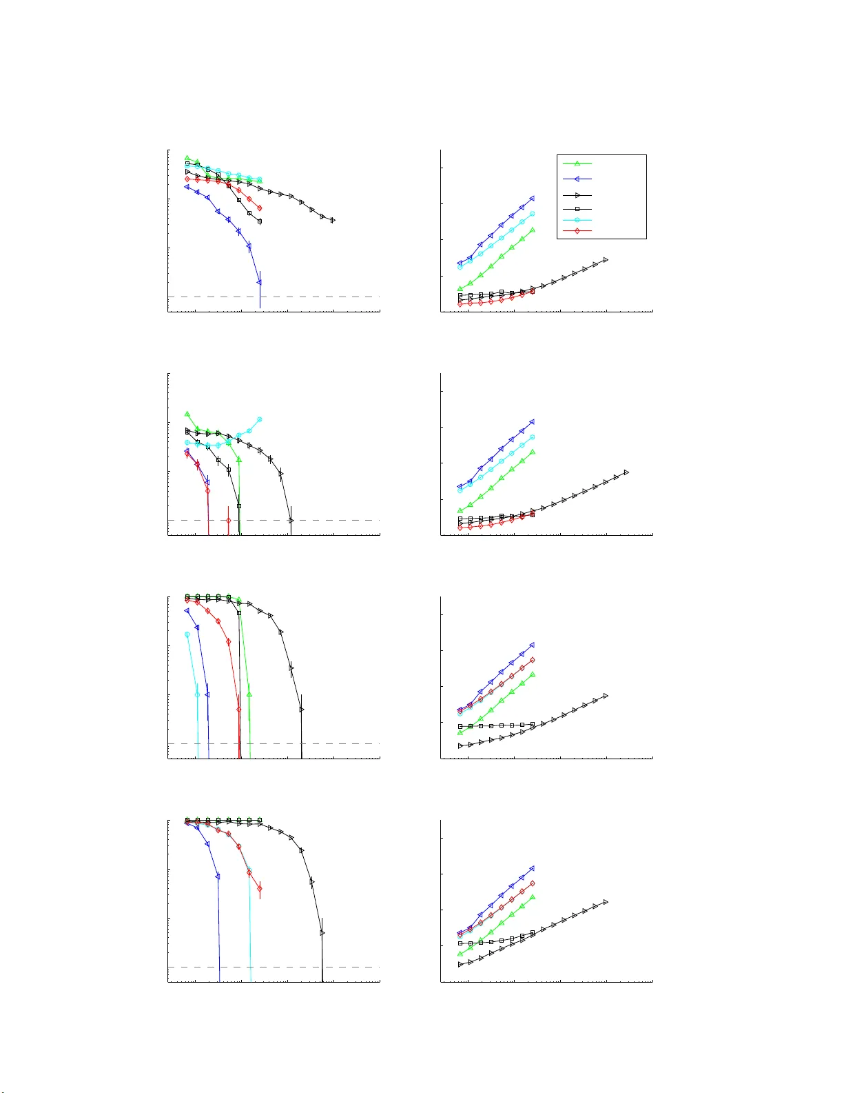
Journal of Mac hine Learning Researc h 1 (2008) 1-10 Submitted 04/08; Published 04/08 A Kernel Metho d for the Tw o-Sample Problem Arth ur Gretton ar thur@tuebingen.mpg.de MPI for Biolo gic al Cyb ernetics Sp emannstr asse 38 72076 , T¨ ubingen, Germany Karsten M. Borgw ardt ∗ kmb51@cam.ac.uk University of Cambridge Dep artment of Engine ering T rumpington Str e et, CB2 1PZ Cambridge, Unite d Kingdom Malte J. Rasc h mal te@igi.tu-graz.ac.a t Gr az University of T e chnolo gy Inﬀeldgasse 16b/I 8010 Gr az, A ustria Bernhard Sch¨ olk opf bernhard.schoelkopf@tuebingen.mpg.de MPI for Biolo gic al Cyb ernetics Sp emannstr asse 38 72076 , T¨ ubingen, Germany Alexander Smola alex.smola@gmail. com National ICT Austr alia Canb err a, A CT 0200, Austr alia Editor: TBA Abstract W e propo se a framew ork fo r ana ly zing and comparing distributions, allowing us to design statistical tests to determine if tw o samples a r e drawn fro m diﬀeren t distributions. Our test s tatistic is the larg est diﬀerence in exp ectations over functions in the unit ba ll of a repro ducing kernel Hilb ert space (RKHS). W e present tw o tests based on large deviation bo unds for the test s tatistic, while a third is ba sed on the asy mptotic distr ibution of this statistic. The test statistic can b e computed in qua dratic time, although eﬃcient linear time approximations are av ailable. Several classica l metrics on distributions ar e r eco vered when the function space use d to compute the diﬀerence in ex p ectations is allow ed to be more general (eg. a Banach space). W e apply our tw o- sample tests to a v ariety of pr oblems, including a ttribute matching for databases using the Hunga rian marria ge method, where they pe rform strongly . Excellent p erformance is also obtained when comparing distribu- tions over gr aphs, for which these are the ﬁrst suc h tests. Keyw ords: Kernel metho ds, t wo sample test, uniform conv er gence bounds, schema matching, a symptotic analysis, h yp othesis testing. ∗ . This work was carried out while K.M.B . was with the Ludwig-Maximilians-Universit¨ at M ¨ unchen. c  2008 Gretton, Borgw ardt, Rasch, Sch¨ olko pf and Smola. Gretton, Bor gw ardt, Rasch, Sch ¨ olkopf and Smola 1. In tro duction W e address the problem of comparing samp les from t wo probability distribu tio ns, b y prop os- ing statistical tests of the h yp othesis that these distribu tions are diﬀeren t (this is called the t wo-sample or homogeneit y problem). Su c h tests ha v e applicat ion in a v ariet y of areas. In bioinformatics, it is of in terest to compare microarray data from identica l ti ssue typ es as measured b y diﬀeren t laboratories, to detec t whether the data ma y b e analysed join tly , or whether diﬀerences in exp erimental pro cedure hav e caused systematic d iﬀerences in th e data distributions. Equally of in terest are comparisons b et w een microarray data from diﬀerent tissue t yp es, either to determine wh ether tw o subtyp es of cancer ma y b e treated as sta- tistically indistinguishable f rom a diagnosis p ersp ectiv e, or to detec t diﬀerences in healthy and cancerous tissue. In d atabase attribute matc hing, it is d esirable to merge d ata bases con taining m ultiple ﬁelds, where it is not kn o wn in adv ance whic h ﬁelds corresp ond: the ﬁelds are matc hed b y maximising the similarit y in the d istributions of their entries. W e test whether distributions p and q are diﬀerent on the basis of samples dra wn from eac h of them, by ﬁ nding a we ll b eha v ed (e.g. smo oth) f unction w hic h is large on the p oints dra wn from p , and small (as negativ e as p ossible) on the p oints fr om q . W e use as our test statistic the d iﬀerence b et w een the mean function v alues on the t w o samples; when this is large, th e samples are like ly fr om diﬀerent distributions. W e call this statistic the Maxim um Mean Discrepancy (MMD ). Clearly the qualit y of the MMD as a statistic dep ends on the class F of smo oth functions that deﬁne it. On one hand, F m ust b e “ric h enough” so that the p opulation MMD v anishes if and only if p = q . On the other hand, for th e test to b e co nsistent, F needs to b e “restrictiv e” enough for the empirical estimate of MMD to con verge quic kly to its exp ectat ion as the sample size increases. W e sh al l use the un it balls in unive rsal repro ducing k ernel Hilb ert spaces (Stein w art, 2001) as our function classes, s ince these will b e sho wn to satisfy b oth of the foregoing prop erties (w e also r evie w classical metrics on d istributions, namely the Kolmogoro v-S mirno v and Earth-Mo ver’s d istance s, wh ic h are b ased on diﬀerent function classes). On a more practical n ote , the MMD has a reasonable computational cost, when compared with other t w o-sample tests: giv en m p oin ts sampled from p and n from q , th e cost is O ( m + n ) 2 time. W e also prop ose a less statistica lly eﬃcien t algorithm with a compu tat ional cost of O ( m + n ), which can yield sup erior p erform an ce at a giv en computational cost b y looking at a larger v olume of data. W e deﬁne three non-parametric statistical tests based on the MMD. The ﬁrst t wo, which use distribution-ind epend en t un iform con vergence b ounds, pro vide ﬁnite sample guarante es of test p erformance, at the exp ense of b eing conserv ativ e in detecting diﬀeren ces b et ween p and q . The third test is based on the a symptotic distr ib ution of th e MMD, and is in practice more sensitiv e to diﬀerences in distribution at small sample sizes. The present w ork synt hesizes and expands on results of Gretton et al. (2007a ,b ), Smola et al. (2007), and Song et al. (2008) 1 who in turn build on the earlier w ork of Borgw ardt et al. (2006). Not e that the latter add resses only the third kind of test, and that the app r oa c h of Gretton et al. (2007 a ,b) emplo ys a more accurate appr o ximation to the asymptotic d istr ibution of the test statistic. 1. In particular, most of the proofs h ere were not provided by Gretton et al. (2007a) 2 A Kernel Method f or the Two-Sample Problem W e b egin our presen tation in Section 2 with a formal deﬁn iti on of the MMD, and a pro of that the p opulation MMD is zero if and only if p = q wh en F is the u nit ball of a unive rsal RKHS. W e also review alternativ e fu nction classes for whic h the MMD deﬁnes a metric on probabilit y distribu tio ns. In Section 3, we give an o ve rview of hyp othesis testing as it applies to the t w o-sample problem, and review other approac h es to this problem. W e present our ﬁrst t wo hypothesis tests in Sectio n 4, based on tw o diﬀeren t b ounds on the deviation b et we en the p opulation and emp ir ica l MMD. W e tak e a diﬀeren t approac h in Section 5, where w e use the asymptotic distrib u tion of the empirical MMD estimate as the basis for a third test. When large v olumes of data are a v ailable, the cost of computing the MMD (quadratic in th e sample size) ma y b e excessiv e: w e therefore prop ose in Section 6 a mo diﬁed version of the MMD statistic th at has a lin ear cost in the num b er of samples, and an asso ciate d asymptotic test. In Section 7, we provide an o verview of metho ds re- lated to the MMD in the statistics and machine learning literature. Finally , in Section 8, w e demonstrate the p erformance of MMD-based tw o-sample tests on problems from neu- roscience, bioinformatics, and attribute matc hing using the Hun ga rian marriage metho d. Our appr oa c h p erform s w ell on high dimensional data with low sample size; in add itio n, w e are able to successfully d istinguish distributions on graph d at a, for which ours is th e ﬁrst prop osed test. 2. The Maxim um Mean Discrepancy In this section, w e present the maxim um mean discrepancy (MMD), and describ e conditions under which it is a metric on the space of probabilit y distributions. The MMD is deﬁned in terms of particular fu n ctio n spaces that witness th e d iﬀerence in distribu tions: we therefore b egin in S ect ion 2.1 by introd ucing th e MMD for some arbitrary function space. In Section 2.2, w e compute b oth the p opulation MMD and t wo empirical estimates when the asso ciated function sp ace is a repro ducing kernel Hilb ert s p ace , and we deriv e the RKHS fun ction that witnesses the MMD f or a giv en pair of distributions in Section 2.3. Finally , we describ e the MMD for more general function classes in Section 2.4. 2.1 Deﬁnition of the Maxim um Mean Discrepancy Our goal is to formulate a statistical test that answe rs th e follo wing question: Problem 1 L et p and q b e Bor el pr ob ability me asur es deﬁne d on a domain X . Given observations X := { x 1 , . . . , x m } and Y := { y 1 , . . . , y n } , dr awn indep endently and identic al ly distribute d (i.i.d.) fr om p and q , r esp e ctively, c an we de cide whether p 6 = q ? T o start with, we wish to determine a crite rion that, in the p opulatio n setting, tak es on a unique and distinctiv e v alue only when p = q . It will b e d eﬁned based on Lemma 9.3.2 of Dudley (2002). Lemma 1 L et ( X , d ) b e a metric sp ac e, and let p, q b e two Bor el pr ob ability me asur es deﬁne d on X . Then p = q if and only if E x ∼ p ( f ( x )) = E y ∼ q ( f ( y )) for al l f ∈ C ( X ) , wher e C ( X ) is the sp ac e of b ounde d c ontinuous functions on X . Although C ( X ) in principle allo ws us to id en tify p = q uniquely , it is not p racti cal to wo rk with suc h a ric h fun ction class in the ﬁnite sample setting. W e th us deﬁne a more general 3 Gretton, Bor gw ardt, Rasch, Sch ¨ olkopf and Smola class of statistic, for as yet unsp eciﬁed fu n ctio n classes F , to measure the disparit y b et we en p and q (F ortet and Mourier, 1953; M ¨ uller, 1997). Deﬁnition 2 L et F b e a class of fu nctions f : X → R and let p , q, X , Y b e deﬁne d as ab ove. We deﬁne the maxim um me an discr ep ancy (MMD) as MMD [ F , p, q ] := su p f ∈ F ( E x ∼ p [ f ( x )] − E y ∼ q [ f ( y )]) . (1) M¨ ul ler (1997) c al ls this an inte gr al pr ob ability metric. A biase d empiric al estimate of the MMD is MMD b [ F , X , Y ] := sup f ∈ F 1 m m X i =1 f ( x i ) − 1 n n X i =1 f ( y i ) ! . (2) The empir ica l MMD deﬁn ed ab o v e has an up ward bias (w e will deﬁne an un biased statistic in the follo wing section). W e m ust no w id en tify a function class that is rich enough to uniquely iden tify whether p = q , y et restrictiv e enough to pr ovide us eful ﬁnite sample estimates (the latt er prop ert y w ill b e established in subsequen t sections). 2.2 The MMD in Repro ducing Kernel Hilb ert Spaces If F is the unit b all in a r ep rodu cing k ernel Hilb ert space H , the empirical MMD can b e computed v ery eﬃcien tly . Th is will b e the main approac h w e pursue in the presen t study . Other p ossible function classes F are discussed at the end of this section. W e will refer to H as univ ers al whenev er H , deﬁn ed on a compact metric space X and with asso ciated kernel k : X 2 → R , is dense in C ( X ) with resp ect to the L ∞ norm. It is shown in Stein wart (2001 ) that Gaussian and Laplace ke rnels are univ ersal. W e ha ve the follo wing result: Theorem 3 L et F b e a unit b al l in a universal RKHS H , deﬁne d on the c omp act metric sp ac e X , with asso ciate d kernel k ( · , · ) . Then MMD [ F , p, q ] = 0 if and only if p = q . Pro of It is clea r that MM D [ F , p, q ] is zero if p = q . W e pro ve the conv erse b y showing that MMD [ C ( X ) , p, q ] = D for some D > 0 imp lies MMD [ F , p, q ] > 0: this is equ iv alen t to MMD [ F , p, q ] = 0 imp lying MMD [ C ( X ) , p, q ] = 0 (wher e this last result implies p = q b y Lemma 1, noting that compactness of the metric space X imp lies its separabilit y). Let H b e the univ ersal RKHS of w hic h F is th e un it ball. If MMD [ C ( X ) , p, q ] = D , then there exists some ˜ f ∈ C ( X ) for which E p h ˜ f i − E q h ˜ f i ≥ D / 2. W e kno w th at H is d ense in C ( X ) w ith resp ect to the L ∞ norm: this means that for ǫ = D / 8, we can ﬁ nd some f ∗ ∈ H satisfying    f ∗ − ˜ f    ∞ < ǫ . Thus, w e obtain    E p [ f ∗ ] − E p h ˜ f i    < ǫ and consequen tly | E p [ f ∗ ] − E q [ f ∗ ] | >    E p h ˜ f i − E q h ˜ f i    − 2 ǫ > D 2 − 2 D 8 = D 4 > 0 . Finally , using k f ∗ k H < ∞ , w e ha ve [ E p [ f ∗ ] − E q [ f ∗ ]] / k f ∗ k H ≥ D / (4 k f ∗ k H ) > 0 , and hence MMD [ F , p, q ] > 0. 4 A Kernel Method f or the Two-Sample Problem W e n o w review some pr operties of H th at will allo w us to express the MMD in a m ore easily computable form (Sc h¨ olk opf and Smola, 2002). Since H is an RKHS , the op erator of ev aluation δ x mapping f ∈ H to f ( x ) ∈ R is con tin uous. Thus, by the Riesz repr esen- tation theorem, there is a feature mapping φ ( x ) from X to R suc h that f ( x ) = h f , φ ( x ) i H . Moreo ve r, h φ ( x ) , φ ( y ) i H = k ( x, y ), wh er e k ( x, y ) is a p ositiv e deﬁnite kernel fu nction. Th e follo wing lemma is due to Borgw ardt et al. (2006). Lemma 4 Denote the exp e ctation of φ ( x ) by µ p := E p [ φ ( x )] (assuming its exi stenc e). 2 Then MMD[ F , p , q ] = sup k f k H ≤ 1 h µ [ p ] − µ [ q ] , f i = k µ [ p ] − µ [ q ] k H . (3) Pro of MMD 2 [ F , p , q ] = " sup k f k H ≤ 1 ( E p [ f ( x )] − E q [ f ( y )]) # 2 = " sup k f k H ≤ 1 ( E p [ h φ ( x ) , f i H ] − E q [ h φ ( y ) , f i H ]) # 2 = " sup k f k H ≤ 1 h µ p − µ q , f i H # 2 = k µ p − µ q k 2 H Giv en w e are in an RKHS, the norm k µ p − µ q k 2 H ma y easily b e computed in terms of kernel functions. Th is leads to a ﬁ rst empirical estimate of the MMD, whic h is unbiased. Lemma 5 Given x and x ′ indep endent r andom variables with distribution p , and y and y ′ indep endent r andom variables with distribution q , the p opulation MMD 2 is MMD 2 [ F , p , q ] = E x,x ′ ∼ p  k ( x, x ′ )  − 2 E x ∼ p,y ∼ q [ k ( x, y )] + E y , y ′ ∼ q  k ( y , y ′ )  . (4) L et Z := ( z 1 , . . . , z m ) b e m i.i.d. r andom v ar iables, wher e z i := ( x i , y i ) (i.e. we assume m = n ). An un biased empiric al estimate of MMD 2 is MMD 2 u [ F , X, Y ] = 1 ( m )( m − 1) m X i 6 = j h ( z i , z j ) , (5) which is a one- sam ple U-statistic with h ( z i , z j ) := k ( x i , x j ) + k ( y i , y j ) − k ( x i , y j ) − k ( x j , y i ) (we deﬁne h ( z i , z j ) to b e symmetric in its ar guments due to r e quir ements that wil l arise i n Se ction 5). Pro of Starting from the expression for MMD 2 [ F , p , q ] in Lemma 4, MMD 2 [ F , p , q ] = k µ p − µ q k 2 H = h µ p , µ p i H + h µ q , µ q i H − 2 h µ p , µ q i H = E p  φ ( x ) , φ ( x ′ )  H + E q  φ ( y ) , φ ( y ′ )  H − 2 E p,q h φ ( x ) , φ ( y ) i H , 2. A suﬃcien t condition for this is k µ p k 2 H < ∞ , whic h is rearranged as E p [ k ( x , x ′ )] < ∞ , where x and x ′ are indep enden t rand om v ariables dra wn according to p . In other wo rds, k is a trace class op erator with respect t o the measure p . 5 Gretton, Bor gw a rdt, Rasch, Sch ¨ olkopf and Smola −6 −4 −2 0 2 4 6 −0.4 −0.2 0 0.2 0.4 0.6 0.8 1 Witness f for Gauss and Laplace densities X Prob. density and f f Gauss Laplace Figure 1: Illustration of th e function maximizing the mean discrepan cy in th e case where a Gaussian is b eing compared with a Laplace distribu tion. Both distribu tions ha v e zero mean and unit v ariance. The function f that witnesses the MMD has b een scaled for p lotting purp oses, and w as computed empirically on the basis of 2 × 10 4 samples, u sing a Gaussian ke rnel with σ = 0 . 5. The pro of is completed by applying h φ ( x ) , φ ( x ′ ) i H = k ( x, x ′ ); the emp ir ica l estimate f oll o ws straigh tforwardly . The empirical statisti c is an unbiased estimate of MMD 2 , although it do es not ha v e mini- m um v ariance, since we are ignoring the cross-terms k ( x i , y i ) of whic h there are only O ( n ). The minimum v ariance estimate is almost iden tical, though (Serﬂing, 1980, S ec tion 5.1.4). The biased stati stic in (2) ma y also b e easily computed follo w ing the ab o v e reasoning. Substituting the empirical estimates µ [ X ] := 1 m P m i =1 φ ( x i ) and µ [ Y ] := 1 n P n i =1 φ ( y i ) of the feature sp ac e means based on resp ectiv e samples X and Y , we obtain MMD b [ F , X , Y ] =   1 m 2 m X i,j =1 k ( x i , x j ) − 2 mn m,n X i,j =1 k ( x i , y j ) + 1 n 2 n X i,j =1 k ( y i , y j )   1 2 . (6) In tuitiv ely w e exp ect the empirical test statistic MMD[ F , X , Y ], whether biased or un- biased, to b e small if p = q , and large if the distrib utions are f ar apart. It costs O (( m + n ) 2 ) time to compu te b oth statistics. Finally , we note th at Harc haoui et al. (2008) recen tly prop osed a mo diﬁcation of the k ernel MMD statistic in Lemma 4, by scaling the feature space mean distance using th e in v erse within-samp le co v ariance op erator, thus emplo ying the k ernel Fisher discriminant as a statistic for testing homogeneit y . This s ta tistic is sho wn to b e r ela ted to th e χ 2 div ergence. 2.3 Witness F unction of the MMD for RKHSs It is al so instru cti v e to consider the witness f which is c hosen by MMD to exhibit the maxim um discrepancy b et ween the t wo distributions. The p opulation f and its empirical 6 A Kernel Method f or the Two-Sample Problem estimate ˆ f ( x ) are r espectiv ely f ( x ) ∝ h φ ( x ) , µ [ p ] − µ [ q ] i = E x ′ ∼ p [ k ( x, x ′ )] − E x ′ ∼ q [ k ( x, x ′ )] ˆ f ( x ) ∝ h φ ( x ) , µ [ X ] − µ [ Y ] i = 1 m P m i =1 k ( x i , x ) − 1 n P n i =1 k ( y i , x ) . This follo w s from the fact that the u nit v ector v m aximiz ing h v , x i H in a Hilb ert space is v = x/ k x k . W e illustrate the b eha vior of MMD in Figure 1 u s ing a one-dimensional example. The data X and Y were generated from distributions p and q with equal means and v ariances, with p Gaussian and q Laplacian. W e c hose F to b e the u nit ball in an RKHS using the Gaussian ke rnel. W e observ e that the fu nctio n f that witnesses the MMD — in other w ords, the function maximizing the mean discrepancy in (1) — is smo oth, p ositiv e where the Laplace density exceeds the Ga ussian densit y (at the cen ter and tai ls), and nega tiv e where the Gaussian densit y is larger. Moreo ver, the magnitude of f is a direct reﬂectio n of the amount by whic h one density exceeds th e other, insofar as th e smo othness constrain t p ermits it. 2.4 The MMD in Other F unction Cla sses The deﬁnition of th e maximum mean discrep an cy is by no means limited to RKHS. In fact, an y fun cti on class F that comes w ith un iform conv ergence guarant ees and is su ﬃcien tly p o werful will enj o y th e abov e prop erties. Deﬁnition 6 L et F b e a subset of some ve ctor sp ac e. The star S [ F ] of a set F is S [ F ] := { αx | x ∈ F and α ∈ [0 , ∞ ) } Theorem 7 Denote by F the subset of some v e ctor sp ac e of functions f r om X to R for which S [ F ] ∩ C ( X ) is dense in C ( X ) with r esp e ct to the L ∞ ( X ) norm. Then MMD [ F , p, q ] = 0 if and only if p = q . Mor e over, under the ab ove c onditions MMD[ F , p, q ] is a metric on the sp ac e of pr ob ability distributions. Whenever the star of F is not dense, MMD is a pseudo-metric sp ac e. 3 Pro of The ﬁrst part of the pro of is almost iden tical to that of T heorem 3 and is therefore omitted. T o see the second part, w e only n eed to prov e the triangle inequalit y . W e ha v e sup f ∈ F | E p f − E q f | + sup g ∈ F | E q g − E r g | ≥ sup f ∈ F [ | E p f − E q f | + | E q f − E r | ] ≥ su p f ∈ F | E p f − E r f | . The ﬁrst part of the theorem establishes that MMD[ F , p, q ] is a metric, since only for p = q do we ha ve MMD[ F , p, q ] = 0. Note that any uniform conv ergence statemen ts in terms of F allo w us immed iately to c h ar- acterize an estimator of MMD( F , p, q ) explicitly . T he follo wing result sho w s ho w (we will reﬁne this reasoning for the RKHS case in Secti on 4). 3. According to D udley (2002 , p . 26) a metric d ( x, y ) satisﬁes th e follo wing four properties: symmetry , triangle inequ ality , d ( x, x ) = 0, and d ( x, y ) = 0 = ⇒ x = y . A pseudo-metric only satisﬁes the ﬁ rst three prop erties. 7 Gretton, Bor gw a rdt, Rasch, Sch ¨ olkopf and Smola Theorem 8 L et δ ∈ (0 , 1) b e a c onﬁdenc e level and assume that for some ǫ ( δ , m, F ) the fol lowing holds for samples { x 1 , . . . , x m } dr awn fr om p : Pr ( sup f ∈ F      E p [ f ] − 1 m m X i =1 f ( x i )      > ǫ ( δ, m, F ) ) ≤ δ. (7) In this c ase we have that Pr {| MMD[ F , p, q ] − MMD b [ F , X , Y ] | > 2 ǫ ( δ / 2 , m, F ) } ≤ δ. (8) Pro of The p roof w orks s imply b y using conv exit y and su p rema as follo ws: | MMD[ F , p, q ] − MMD b [ F , X , Y ] | =      sup f ∈ F | E p [ f ] − E q [ f ] | − su p f ∈ F      1 m m X i =1 f ( x i ) − 1 n n X i =1 f ( y i )           ≤ sup f ∈ F      E p [ f ] − E q [ f ] − 1 m m X i =1 f ( x i ) + 1 n n X i =1 f ( y i )      ≤ sup f ∈ F      E p [ f ] − 1 m m X i =1 f ( x i )      + su p f ∈ F      E q [ f ] − 1 n n X i =1 f ( y i )      . Bounding eac h of the tw o terms via a un iform con v ergence b ound prov es the cla im. This s h o ws that MMD b [ F , X , Y ] can b e used to estimate MMD[ F , p, q ] and that the qu an tit y is asymptotically un biased. Remark 9 (Reduction t o Binary Classiﬁcation) Any classiﬁer which maps a set of observations { z i , l i } with z i ∈ X on some domain X and lab els l i ∈ {± 1 } , for which u niform c onver genc e b ounds exist on the c onver genc e of the e mp iric al loss to the exp e cte d loss, c an b e use d to obtain a similarity me asur e on distributions — simply assign l i = 1 if z i ∈ X an d l i = − 1 for z i ∈ Y and ﬁnd a classiﬁer which is able to sep ar ate the two sets. In this c ase maximization of E p [ f ] − E q [ f ] is achieve d by ensuring that as many z ∼ p ( z ) as p ossible c orr esp ond to f ( z ) = 1 , wher e as for as many z ∼ q ( z ) as p ossible we have f ( z ) = − 1 . Conse qu ently neur al netwo rks, de cision tr e es, b o oste d classiﬁers and other obje cts for which uniform c onver genc e b ounds c an b e obtaine d c an b e use d for the purp ose of distribution c omp arison. F or i nsta nc e, Ben-David et al. (2007, Se c tion 4) use the e rr or of a hyp erplane classiﬁer to appr oximate the A -distanc e b etwe e n distributions of Kifer et al. (20 04). 2.5 Examples of Non-RKHS F unction C lasses Other f unction spaces F inspired by the statistics literature can also b e considered in deﬁning the MMD. I ndeed, Lemma 1 d eﬁnes an MMD with F the space of b ounded con tinuous real- v alued functions, which is a Banac h sp ace with the sup rem um n orm (Dud ley, 2002, p. 158). W e no w d escribe t w o further metrics on the space of probabilit y distributions, the Kolmogoro v-Smirn o v and Earth Mov er’s distances, and th eir asso cia ted f unction classes. 8 A Kernel Method f or the Two-Sample Problem 2.5.1 Kolmogoro v -Smirno v St a tistic The Kolmogoro v-Smirnov (K-S) test is p robably one of the most famous t w o-sample tests in statistics. It wo rks for random v ariables x ∈ R (or an y other set for whic h w e can establish a tota l ord er). Denote b y F p ( x ) the cum ulativ e distribution function of p and let F X ( x ) b e its empir ical coun terpart, that is F p ( z ) := Pr { x ≤ z for x ∼ p ( x ) } and F X ( z ) := 1 | X | m X i =1 1 z ≤ x i . It is clear that F p captures the prop erties of p . The Kolmogoro v metric is simp ly the L ∞ distance k F X − F Y k ∞ for t w o sets of observ ations X an d Y . Smirno v (1939) sho w ed that for p = q the limiting distribution of th e empirical cumulat iv e distrib u tion functions satisﬁes lim m,n →∞ Pr  h mn m + n i 1 2 k F X − F Y k ∞ > x  = 2 ∞ X j =1 ( − 1) j − 1 e − 2 j 2 x 2 for x ≥ 0 . (9) This allo w s for an eﬃcien t charact erization of the distribu tio n under the null hyp othesis H 0 . Eﬃcien t numerical appr o ximations to (9) can b e found in n umerical analysis handb o oks (Press et al. , 1994). T h e distribution under the alternativ e, p 6 = q , how ev er, is unkno wn. The Kolmogoro v metric is, in fact, a sp ecial instance of MMD[ F , p, q ] for a certain Banac h space (M ¨ uller, 1997, Theorem 5.2) Prop osition 10 L et F b e the class of functions X → R of b ounde d variation 4 1. Then MMD[ F , p , q ] = k F p − F q k ∞ . 2.5.2 Ear th-Mover Dist a nces Another class of distance measures on distr ibutions that ma y b e wr itte n as an MMD are the E arth -Mo ver distances. W e assume ( X , d ) is a separable metric sp ace , and deﬁ ne P 1 ( X ) to b e th e space of p robabilit y m easur es on X for w hic h R d ( x, z ) dp ( z ) < ∞ for all p ∈ P 1 ( X ) and x ∈ X (these are the p robabilit y measures for whic h E | x | < ∞ wh en X = R ). W e then ha v e th e follo wing deﬁnition (Dudley, 20 02, p . 420). Deﬁnition 11 (Monge-W asserstein metric) L et p ∈ P 1 ( X ) and q ∈ P 1 ( X ) . The Monge- Wasserstein distanc e is deﬁne d as W ( p, q ) := inf µ ∈ M ( p,q ) Z d ( x, y ) dµ ( x, y ) , wher e M ( p, q ) is the set of joint distributions on X × X with mar ginals p and q . 4. A fun ction f deﬁned on [ a, b ] is of b ounded v ariation C if the total v ariation is boun d ed by C , i.e. the supremum over all sums X 1 ≤ i ≤ n | f ( x i ) − f ( x i − 1 ) | , where a ≤ x 0 ≤ . . . ≤ x n ≤ b (D udley, 2002, p . 184). 9 Gretton, Bor gw a rdt, Rasch, Sch ¨ olkopf and Smola W e m ay inte rpret this as the cost (as repr esented b y the metric d ( x, y )) of transferring mass distributed according to p to a distr ib ution in accordance with q , where µ is th e mov emen t sc h edule. In general, a large v ariet y of costs of mo ving mass from x to y can b e used, suc h as p syc ho optical s imila rit y measures in image retriev al (Rub ner et al., 2000). The follo win g theorem holds (Dudley, 2002, Th eorem 11 .8.2). Theorem 12 (Kantoro vic h-Rubinstein) L et p ∈ P 1 ( X ) and q ∈ P 1 ( X ) , wher e X is sep ar able. Then a metric on P 1 ( S ) i s deﬁne d as W ( p, q ) = k p − q k ∗ L = sup k f k L ≤ 1     Z f d ( p − q )     , wher e k f k L := sup x 6 = y ∈ X | f ( x ) − f ( y ) | d ( x, y ) is the Lipschitz seminorm 5 for r e al value d f on X . A simple example of this theorem is as follo w s (Dudley, 2002, Exercise 1, p. 425). Example 1 L et X = R with asso ciate d d ( x, y ) = | x − y | . Then gi ven f such that k f k L ≤ 1 , we use inte gr ation by p arts to obtain     Z f d ( p − q )     =     Z ( F p − F q )( x ) f ′ ( x ) dx     ≤ Z | ( F p − F q ) | ( x ) dx, wher e the maximum is attaine d for the function g with derivative g ′ = 2 1 F p >F q − 1 (and for which k g k L = 1 ). We r e c over the L 1 distanc e b etwe en distribution functions, W ( P, Q ) = Z | ( F p − F q ) | ( x ) dx. One may furth er generalize Theorem 12 to the set of all laws P ( X ) on arbitrary metric spaces X (Dud ley, 2002, Prop osition 11.3.2). Deﬁnition 13 (Bounded Lipsc hitz metric) L et p and q b e laws on a metric sp ac e X . Then β ( p, q ) := sup k f k BL ≤ 1     Z f d ( p − q )     is a metric on P ( X ) , wher e f b elongs to the sp ac e of b ounde d Lipschitz functions with norm k f k B L := k f k L + k f k ∞ . 3. Bac kground Material W e no w pr esen t three b ac kground resu lts. First, w e introdu ce th e terminology u sed in statistica l h yp othesis testing. Second, w e demons trate via an example that even for tests whic h h a v e asymptotical ly no error, one cannot guarante e p erformance at any ﬁxed sample size without making assumptions ab out the distributions. Fin ally , w e b rieﬂy review some earlier appr oac hes to the tw o-sample problem. 5. A seminorm satisﬁes the requirements of a n orm besides k x k = 0 only for x = 0 (Dud ley, 2002, p. 156). 10 A Kernel Method f or the Two-Sample Problem 3.1 Statistical Hyp othesis T esting Ha ving describ ed a m etric on probability distribu tio ns (the MMD) based on distances b e- t ween their Hilb ert space embedd ings, and empirical estimates (biased and u n b iased) of this metric, w e no w add ress the problem of d ete rmining whether the empirical MMD sh o ws a statistic al ly signiﬁc ant diﬀerence b et ween distributions. T o this end, we brieﬂy describ e the framew ork of statistical hyp ot hesis testing as it app lie s in the present con text, follo win g Casella and Berger (2002, Chapter 8). Giv en i.i.d. samples X ∼ p of size m and Y ∼ q of size n , the statistical test, T ( X , Y ) : X m × X n 7→ { 0 , 1 } is u sed to distinguish b etw een the n ull h yp othesis H 0 : p = q and the alternativ e hypothesis H 1 : p 6 = q . T his is ac hiev ed b y comparing the test statistic 6 MMD[ F , X , Y ] with a p articular thr eshold: if the threshold is exceeded, then the test rejects the n ull hypothesis (b earing in m in d that a zero p opulatio n MMD in d ica tes p = q ). T h e acce ptance region of the test is thus deﬁned as the set of real n umbers b elo w the thresh old. Sin ce the test is based on ﬁn ite samp les, it is p ossible that an incorrect answ er will b e returned : we deﬁn e the T yp e I error as the pr obabilit y of r ejecting p = q b ased on the observed sample, despite the n ull hyp othesis ha ving generated the data. Con v ersely , the T yp e I I error is the probab ility of accepting p = q despite the un derlying distributions b eing diﬀerent. The level α of a test is an upp er b ound on the T yp e I error: this is a design parameter of the test, and is used to set the thr esh old to w hic h w e compare the test statistic (ﬁnding the test th reshold for a giv en α is the topic of Sections 4 and 5) . A consisten t test ac hiev es a lev el α , and a Typ e I I error of zero, in the large sample limit. W e will see that the tests p r oposed in this pap er are consisten t. 3.2 A Negative Result Ev en if a test is consistent, it is n ot p ossible to distinguish distribu tio ns with high probabilit y at a given, ﬁxed sample size (i.e., to p ro vide guarant ees on the Typ e I I error), without p rior assumptions as to the n ature of the diﬀeren ce b et ween p and q . This is true r e gar d less of the t wo-sample test used. There are sev eral wa ys to illus trate this, wh ich eac h giv e diﬀeren t insight into the kind s of d iﬀerences that m ig ht b e und ete ctable for a giv en n u m b er of samples. The follo wing example 7 is one suc h illustration. Example 2 A ssu me that we have a distribution p fr om which we dr aw m iid observa- tions. Mor e over, we c onstruct a distribution q by dr awing m 2 iid observations fr om p and subse quently deﬁning a discr ete distribution over these m 2 instanc es with pr ob ability m − 2 e ach. It i s e asy to che ck that if we now dr aw m observations fr om q , ther e is at le ast a  m 2 m  m ! m 2 m > 1 − e − 1 > 0 . 63 pr ob ability that we ther eb y wil l have eﬀe ctiv ely obtaine d an m sample fr om p . Henc e no test wil l b e able to distinguish sam ples fr om p and q in this c ase. We c ould make the pr ob ability of dete ction arbitr arily smal l by incr e asing the size of the sample fr om which we c onstruct q . 6. This may b e biased or unbiased. 7. This is a v ariation of a construction for indep endence tests, which was suggested in a priv ate communi- cation by John Langford. 11 Gretton, Bor gw a rdt, Rasch, Sch ¨ olkopf and Smola 3.3 Previous W ork W e next giv e a brief o v erview of some earlier approac hes to th e t wo sample problem for m ultiv ariate data. Since our later exp erimenta l comparison is with resp ect to certain of these metho ds, we giv e abb r evia ted algorithm n ames in italics where appropr iate: these sh ould b e used as a k ey to th e tables in Section 8. A generalisation of the W ald-W olfowitz runs test to th e multiv ariate domain wa s prop osed and analysed by F riedman and Rafsky (1979); Henze and P enrose (1999) (FR Wolf ) , and in v olv es coun ting the num b er of edges in the minim um spann ing tree o ver the ag gregated d ata that connect p oint s in X to p oints in Y . The resulting test relies on the asymptotic normalit y of the test statistic, and this quan tity is n ot distribution-free under the n ull h y p othesis for ﬁn ite samples (it dep ends on p and q ). The computational cost of th is metho d using Kr u sk al’s algorithm is O (( m + n ) 2 log( m + n )), although more mo dern metho ds improv e on the log( m + n ) term. S ee Chazelle (2000) for details. F riedman and Rafsky (1979) claim that calculating the matrix of distances, whic h costs O (( m + n ) 2 ), d omin at es their computing time; we return to this p oin t in our exp erimen ts (Section 8 ). Tw o p ossible generalisations of the Kolmogoro v-S mirno v test to the m ultiv ariate case were studied in (B ic k el , 1969; F riedman and Rafsky, 1979). The approac h of F r iedm an and Rafsky (FR Smirnov) in this case again requires a m inimal spanning tree, and has a similar cost to their m u ltiv ariate r uns test. A more recent multiv ariate test wa s in tro duced b y Rosen baum (2005). This entai ls computing the minim um distance non-bipartite matc hing o ve r the aggreg ate data, and using the num b er of pairs con taining a sample from b oth X and Y as a test statistic . Th e resu lting statistic is d istribution-free under the null h yp othesis at ﬁn ite sample sizes, in wh ic h resp ect it is s up erior to th e F riedman-Rafsky test; on th e other hand, it costs O (( m + n ) 3 ) to compute. Another distribution-free test (Hal l) wa s prop osed by Hall and T a jvidi (20 02): for eac h p oint f rom p , it requ ir es computing the closest p oin ts in the aggregate d data, and coun ting h ow many of these are from q (the p rocedur e is repeated for eac h p oin t from q with resp ect to p oin ts from p ). As w e shall see in our exp erimen tal comparisons, the test statistic is costly to compute; Hall and T a jvid i (2002) consider only tens of p oin ts in their exp erimen ts. Y et another app roac h is to u se s ome distance (e.g. L 1 or L 2 ) b et w een P arzen win do w estimates of the densities as a test s tatistic (And erson et al., 1994; Biau and Gyorﬁ, 2005), based on the asymptotic d istribution of this distance giv en p = q . When th e L 2 norm is used, the test statistic is related to those we present here, although it is arr iv ed at from a diﬀerent p ersp ecti v e. Brieﬂy , the test of Anderson et al. (1994) is obtained in a more restricted setting where the RKHS kernel is an inner pro duct b et ween Pa rzen win do ws. Since we are not doing densit y estimation, h o w ev er, we need not decrease the ke rnel width as the sample gro ws. In fact, decreasing th e k ernel width r educes the conv ergence r at e of the asso ciate d t wo -sample test, compared with the ( m + n ) − 1 / 2 rate for ﬁ x ed k ern els. W e pro vide m ore detail in Sectio n 7.1. T h e L 1 approac h of Biau and Gy orﬁ (2005) (Biau) requires the space to b e partitioned into a grid of bins , w hic h b ecomes diﬃcult or imp ossible for high dimensional p roblems. Hence we use this test only for lo w -dimensional p roblems in our experiments. 12 A Kernel Method f or the Two-Sample Problem 4. T ests Based on Uniform Conv ergence Bounds In this sect ion, we int ro duce t w o statist ical te sts of indep endence whic h h a v e exact p erfor- mance guaran tees at ﬁn ite sample sizes, based on un if orm conv ergence b ounds. The ﬁrst, in Section 4.1 , uses the McDiarmid (1989) b ound on the biased MMD statistic, and the second, in Sectio n 4.2, uses a Ho eﬀding (19 63) b ound for the unbiased statistic. 4.1 Bound on the Biased Statistic and T est W e establish tw o prop erties of the MMD, from wh ic h we derive a h yp othesis test. First, w e sho w that rega rdless of whether or not p = q , th e empirical MMD conv erges in probabilit y at rate O (( m + n ) − 1 2 ) to its p opulation v alue. This sho ws the consistency of statistical tests based on th e MMD. Second, we giv e pr ob ab ilistic b ounds for large deviations of the empirical MMD in th e case p = q . These b ounds lead directly to a threshold for ou r ﬁrst hyp othesis test. W e b egin our d iscussion of the con vergence of MMD b [ F , X , Y ] to MMD[ F , p , q ]. Theorem 14 L et p, q , X , Y b e deﬁne d as in Pr oblem 1, and assume 0 ≤ k ( x, y ) ≤ K . Then Pr n | MMD b [ F , X , Y ] − MMD [ F , p, q ] | > 2  ( K/m ) 1 2 + ( K /n ) 1 2  + ǫ o ≤ 2 exp  − ǫ 2 mn 2 K ( m + n )  . See App endix A.2 for pro of. Our next goal is to reﬁne this resu lt in a wa y that allo ws us to deﬁn e a test th reshold under the null h yp othesis p = q . Under this circumstance, the constan ts in the expon ent are sligh tly impro ved. Theorem 15 U nder the c onditions of The or em 14 wher e additional ly p = q and m = n , MMD b [ F , X , Y ] ≤ m − 1 2 q 2 E p [ k ( x, x ) − k ( x, x ′ )] | {z } B 1 ( F ,p ) + ǫ ≤ (2 K/m ) 1 / 2 | {z } B 2 ( F ,p ) + ǫ, b oth with pr ob ability at le ast 1 − exp  − ǫ 2 m 4 K  (se e App endix A.3 for the pr o of ). In this theorem, we illustrate t wo p ossible b ounds B 1 ( F , p ) and B 2 ( F , p ) on the bias in the empirical estimate (6). The ﬁrst in equ ali t y is inte resting inasm uc h as it pro vides a link b et ween the bias b ound B 1 ( F , p ) and k ernel size (for instance, if w e w ere to use a Gaussian k ernel with large σ , then k ( x, x ) and k ( x, x ′ ) w ould lik ely b e close, and the bias small). In the con text of testi ng, ho w ev er, w e w ould need to provide an additional b ound to sh o w con vergence of an empirical estimate of B 1 ( F , p ) to its p opu lat ion equiv alent . Thus, in the follo wing test for p = q based on Theorem 15, we use B 2 ( F , p ) to b ound the b ias. 8 Corollary 16 A hyp othesis test of level α for the nul l hyp othesis p = q , that i s, for MMD[ F , p , q ] = 0 , ha s the ac c eptanc e r e gion MMD b [ F , X , Y ] < p 2 K/m  1 + p 2 log α − 1  . W e emphasise that Theorem 14 guarantees the consistency of the test, and that the Typ e I I error probabilit y decreases to zero at rate O ( m − 1 2 ), assum ing m = n . T o p ut this con- v ergence rate in p ersp ectiv e, consider a test of whether tw o n ormal distr ib utions ha v e equal 8. Note that we use a tighter b ia s b ound than Gretton et al. (2007a). 13 Gretton, Bor gw a rdt, Rasch, Sch ¨ olkopf and Smola means, given they ha ve u n kno wn but equal v ariance (Casella and Berger , 2002, Exercise 8.41). In this case, the test statistic has a Student- t distribution with n + m − 2 degrees of freedom, and its error prob ab ility con verges at th e same rate as our test. It is w orth n oting that b ounds ma y b e obtained for the deviation b et w een exp ectatio ns µ [ p ] and th e empirical means µ [ X ] in a completely analogous fashion. The pro of requires symmetrization by means of a g host sample , i.e. a second set of o bserv ations d ra wn from the same distribution. While not th e k ey fo cus of the present pap er, suc h b ound s can b e used in the design of inference principles based on moment mat c hing (Altun and Smola, 2006; Dud ´ ık and S c hapire, 200 6; Dud ´ ık et al., 2004). 4.2 Bound on the Unbiased St atistic and T est While the previous b oun ds are of in terest since the pr o of strateg y can b e used for general function classes with wel l b eha ved Rademac her a v erages, a muc h easier approac h ma y b e used directly on the unbiased statistic MMD 2 u in Lemma 5. W e base our test on the f oll o wing theorem, wh ic h is a straigh tforw ard ap p lica tion of th e large deviation b ound on U-statistics of Ho eﬀding (1963, p. 25). Theorem 17 A ssume 0 ≤ k ( x i , x j ) ≤ K , fr om which it fol lows − 2 K ≤ h ( z i , z j ) ≤ 2 K . Then Pr  MMD 2 u ( F , X , Y ) − MMD 2 ( F , p, q ) > t  ≤ exp  − t 2 m 2 8 K 2  wher e m 2 := ⌊ m/ 2 ⌋ (the same b ound applies for deviations of − t and b elow). A consisten t stati stical test for p = q u sing MMD 2 u is then obtained. Corollary 18 A hyp othesis test of level α f or the nul l hyp othesis p = q has the ac c eptanc e r e gion MMD 2 u < (4 K/ √ m ) p log( α − 1 ) . W e n o w compare the thresholds of the t wo tests. W e note ﬁr st that th e threshold for the biased statistic applies to an estimate of MMD, whereas that for the unbiased statistic is for an estimate of MMD 2 . Squaring the former threshold to mak e the t w o qu an tities comparable, the squared thresh old in Corollary 16 decreases as m − 1 , w hereas the threshold in Corollary 18 decreases as m − 1 / 2 . Thus for su ﬃcien tly large 9 m , the McDiarmid-based threshold will b e lo wer (and the asso ciated test statistic is in any case biased upw ards), and its Typ e I I error will b e b etter for a giv en T yp e I b ound. T his is conﬁrm ed in our Sectio n 8 exp erimen ts. Note, ho we v er, that the rate of conv ergence of the squared , biased MMD estimate to its p opulation v alue remains at 1 / √ m (b earing in mind we ta k e the square of a biased esti mate, where the bias term deca ys as 1 / √ m ). Finally , we note that th e b ounds we obtained here are rather conserv ativ e for a n umb er of reasons: ﬁrst, they d o not tak e the actual d istributions into accoun t. In fact, they are ﬁnite samp le size, distribution free b ound s that hold ev en in the w orst case s cenario. The b ounds could b e tigh tened using lo cali zation, momen ts of the distrib ution, etc. An y suc h impr o v emen ts could b e plugged str aight into Theorem 8 for a tigh ter b ound. See e.g . Bousquet et al. (2005) for a d eta iled d iscussion of recen t uniform con vergence b oundin g 9. In the case of α = 0 . 05, this is m ≥ 12. 14 A Kernel Method f or the Two-Sample Problem metho ds. Second, in compu ting b ounds rather than tryin g to charact erize the distribution of MMD( F , X , Y ) explicitly , we force our test to b e conserv ativ e b y d esign. In the follo wing w e aim for an exact c h arac terization of the asymptotic distribution of MMD( F , X , Y ) instead of a boun d. While this will n ot satisfy the uniform con v ergence r equiremen ts, it leads to sup erior tests in practice . 5. T est B ase d on the Asymptotic Distribution of the Un biased Statistic W e no w prop ose a th ird test, whic h is based on the asymptotic distribution of the unbiased estimate of MMD 2 in Lemma 5 . Theorem 19 W e assume E  h 2  < ∞ . Under H 1 , MMD 2 u c onver ges in distribution (se e e.g. Grimmet and Stirzaker, 200 1 , Se ction 7.2) to a Gaussian ac c or ding to m 1 2  MMD 2 u − MMD 2 [ F , p , q ]  D → N  0 , σ 2 u  , wher e σ 2 u = 4  E z  ( E z ′ h ( z , z ′ )) 2  −  E z ,z ′ ( h ( z , z ′ ))  2  , uniformly at r ate 1 / √ m (Serﬂing , 1980, The or em B, p. 193). U nder H 0 , the U-statistic is de gener ate, me aning E z ′ h ( z , z ′ ) = 0 . In this c ase, MMD 2 u c onver ges in distribution ac c or ding to m MMD 2 u D → ∞ X l =1 λ l  z 2 l − 2  , (10) wher e z l ∼ N (0 , 2) i. i.d., λ i ar e the solutions to the eigenvalue e quation Z X ˜ k ( x, x ′ ) ψ i ( x ) dp ( x ) = λ i ψ i ( x ′ ) , and ˜ k ( x i , x j ) := k ( x i , x j ) − E x k ( x i , x ) − E x k ( x, x j ) + E x,x ′ k ( x, x ′ ) is the c entr e d RKH S kernel. The asymptotic distribution of the test statistic under H 1 is giv en b y Serﬂing (1980, Section 5.5.1), and the distr ib ution u nder H 0 follo ws Serﬂing (1980, Section 5.5.2) and Anderson et al. (1994, App endix); see App endix B.1 for details. W e illustrate the MMD densit y under b oth th e null an d alt ernativ e hyp otheses by ap p ro ximating it empirically for b oth p = q and p 6 = q . Results are plotted in Figure 2. Our go al is to determine w hether the empirical test statistic MMD 2 u is so large as to b e outside the 1 − α qu antile of th e n u ll distribution in (10) (consistency of the resulting test is g uarante ed by the form of the distribution under H 1 ). One w ay to estimate this quan tile is usin g the b o ot strap on the aggreg ated data, follo win g Arcones and Gin ´ e (199 2 ). Alternativ ely , w e ma y app r o ximate the null distribution by ﬁtting Pe arson curv es to its ﬁ rst four momen ts (Johns on et al., 199 4, S ect ion 18.8). T aking adv an tage of the degenerac y of the U-statistic, w e obtain (see App end ix B.2) E   MMD 2 u  2  = 2 m ( m − 1) E z ,z ′  h 2 ( z , z ′ )  and (11) E   MMD 2 u  3  = 8( m − 2) m 2 ( m − 1) 2 E z ,z ′  h ( z , z ′ ) E z ′′  h ( z , z ′′ ) h ( z ′ , z ′′ )  + O ( m − 4 ) . (12) 15 Gretton, Bor gw a rdt, Rasch, Sch ¨ olkopf and Smola −0.04 −0.02 0 0.02 0.04 0.06 0.08 0.1 0 10 20 30 40 50 Empirical MMD density under H0 MMD Prob. density 0.05 0.1 0.15 0.2 0.25 0.3 0.35 0.4 0 2 4 6 8 10 Empirical MMD density under H1 MMD Prob. density Figure 2: Left: Empirical distrib ution of th e MMD und er H 0 , with p and q b oth Gaussians with un it standard d eviation, usin g 50 samples from eac h. Righ t: Empirical distribution of the MMD under H 1 , with p a L aplac e distr ibution w ith unit standard d evia tion, and q a Laplac e d istribution with standard d eviat ion 3 √ 2, using 100 samples from eac h. In b oth ca ses, th e histograms were obtained b y computing 2000 indep enden t instances of the MMD. The fourth moment E   MMD 2 u  4  is not compu ted, since it is b oth v ery small, O ( m − 4 ), and exp ensiv e to calculate, O ( m 4 ). I nstead, w e r ep lac e the kurtosis 10 with a lo wer b ound due to Wilki ns (194 4), kurt  MMD 2 u  ≥  sk ew  MMD 2 u  2 + 1. Note that MMD 2 u ma y b e negativ e, since it is an u nbiased estimator of (MMD[ F , p , q ]) 2 . Ho wev er, the only terms missin g to en s ure nonn ega tivit y are the terms h ( z i , z i ), wh ic h w ere remo ved to remo ve spurious correlati ons b etw een observ ations. Consequ en tly we hav e the b ound MMD 2 u + 1 m ( m − 1) m X i =1 k ( x i , x i ) + k ( y i , y i ) − 2 k ( x i , y i ) ≥ 0 . (13) 6. A Linear Time St atistic and T est While the ab o v e tests are already more eﬃcient than the O ( m 2 log m ) and O ( m 3 ) tests describ ed earlier, it is still desirable to ob tain O ( m ) tests whic h do not sac riﬁce to o m uc h statistica l pow er. Moreo ver, w e w ould lik e to obtain tests whic h ha ve O (1) storage require- men ts for computing th e test statistic in order to apply it to data streams. W e no w d escrib e ho w to ac hiev e this by computing th e test statistic based on a sub s ampling of the terms in the sum. The empirical estimate in this case is obtained b y dr a wing pairs from X and Y resp ectiv ely without replacemen t. 10. The kurtosis is deﬁned in terms of the fourth and second moments as ku rt ` MMD 2 u ´ = E “ [ MMD 2 u ] 4 ” h E “ [ MMD 2 u ] 2 ”i 2 − 3. 16 A Kernel Method f or the Two-Sample Problem Lemma 20 R e c al l m 2 := ⌊ m/ 2 ⌋ . The estimator MMD 2 l [ F , X , Y ] := 1 m 2 m 2 X i =1 h (( x 2 i − 1 , y 2 i − 1 ) , ( x 2 i , y 2 i )) c an b e c ompute d in line ar time. M or e over, it is an unbiase d estimate of MMD 2 [ F , p , q ] . While it is exp ected (as we will see explicitly later) that MMD 2 l has higher v ariance than MMD 2 u , it is computationally m u c h more app ealing. In particular, the statistic can b e u sed in stream computations with need for only O (1) memory , w hereas MMD 2 u requires O ( m ) storage and O ( m 2 ) time to compute the kernel h on all in teracting pairs. Since MMD 2 l is just th e av erage o v er a set of rand om v ariables, Ho eﬀding’s b oun d and the ce ntral limit theo rem readily allo w us to pro vid e b oth uniform con v ergence and asymptotic statemen ts f or it with little eﬀort. Th e ﬁrst follo ws dir ectly from Ho eﬀding (1963, Th eo rem 2). Theorem 21 A ssume 0 ≤ k ( x i , x j ) ≤ K . Then Pr  MMD 2 l ( F , X , Y ) − MMD 2 ( F , p, q ) > t  ≤ exp  − t 2 m 2 8 K 2  wher e m 2 := ⌊ m/ 2 ⌋ (the same b ound applies for deviations of − t and b elow). Note that th e b ound of T heorem 17 is iden tical to that of Theorem 21, whic h s h o ws th e former is r ather lo ose. Next we in v oke th e cen tral limit theorem. Corollary 22 A ssume 0 < E  h 2  < ∞ . Then MMD 2 l c onver ges in distribution to a Gaussian ac c or ding to m 1 2  MMD 2 l − MMD 2 [ F , p , q ]  D → N  0 , σ 2 l  , wher e σ 2 l = 2 h E z ,z ′ h 2 ( z , z ′ ) −  E z ,z ′ h ( z , z ′ )  2 i , uniformly at r ate 1 / √ m . The factor of 2 arises sin ce we are av eraging ov er only ⌊ m/ 2 ⌋ ob s erv ations. Note the diﬀerence in the v ariance b et w een Theorem 19 and Corollary 22, namely in th e former case w e are interested in the a v erage conditional v ariance E z V ar z ′ [ h ( z , z ′ ) | z ], wh er eas in the latter case w e co mpute the full v ariance V ar z ,z ′ [ h ( z , z ′ )]. W e end by n oting another p oten tial approac h to redu cing the computational cost of the MMD, b y computing a lo w rank appr o ximation to the Gram matrix (Fine and Schein b erg, 2001; Williams and Seeger, 2001; Smola and Sc h¨ olk opf , 2000). An incremental computation of the MMD based on such a lo w rank appro ximation w ould require O ( md ) storage and O ( md ) computation (wh ere d is the rank of the approximat e Gr am matrix which is used to factorize b oth matrices) rather than O ( m ) storage and O ( m 2 ) op eratio ns. Th at said, it remains to b e determined what eﬀect this appro ximation w ould ha ve on the distribution of the test stati stic under H 0 , and h ence on the test threshold. 17 Gretton, Bor gw a rdt, Rasch, Sch ¨ olkopf and Smola 7. Simila rity Measures Related to MMD Our main p oin t is to p r opose a new ke rnel statistic to te st wh ether tw o d istr ibutions are the same. Ho we v er, it is reassuring to observ e links to other measures of similarit y b et ween distributions. 7.1 Link with L 2 Distance b etw een P arzen Windo w Estimates In this section, we d emonstrate the connection b et wee n ou r test statistic and the Parzen windo w-based statistic of Anderson et al. (1994 ). W e sho w that a tw o-sample test based on P arzen w indo ws conv erges more slo wly than an RKHS-b ased test, also follo wing Anderson et al. (1994). Before pro ceeding, w e motiv ate this discussion with a short ov erview of the P arzen windo w estimate and its p r operties (Silv erman, 1986). W e assume a distribution p on R d , whic h has an asso ciated density fun ctio n also wr itte n p to minimise notation. The P arzen windo w estimate of this den sit y from an i.i.d. sample X of size m is ˆ p ( x ) = 1 m m X l =1 κ ( x l − x ) w here κ satisﬁes Z X κ ( x ) dx = 1 and κ ( x ) ≥ 0 . W e may rescale κ according to 1 h d m κ  x h m  . Consistency of the P arzen w indo w estimate requires lim m →∞ h d m = 0 and lim m →∞ mh d m = ∞ . (14) W e now sho w that th e L 2 distance b etw een P arzen windows densit y estimates (And er s on et al., 1994) is a sp ecial case of the biased MMD in equation (6). Denote by D r ( p, q ) := k p − q k r the L r distance. F or r = 1 the distance D r ( p, q ) is kno w n as the Levy d ista nce (F eller, 1971), and for r = 2 w e encount er distance measures derived from the R enyi ent ropy (Gok ca y and Pr incipe, 2002 ). Assume that ˆ p and ˆ q are giv en as k ernel densit y estimates with kernel κ ( x − x ′ ), that is, ˆ p ( x ) = m − 1 P i κ ( x i − x ) an d ˆ q ( y ) is deﬁned by analogy . In this case D 2 ( ˆ p, ˆ q ) 2 = Z " 1 m X i κ ( x i − z ) − 1 n X i κ ( y i − z ) # 2 dz (15) = 1 m 2 m X i,j =1 k ( x i − x j ) + 1 n 2 n X i,j =1 k ( y i − y j ) − 2 mn m,n X i,j =1 k ( x i − y j ) , (16) where k ( x − y ) = R κ ( x − z ) κ ( y − z ) dz . By its deﬁnition k ( x − y ) is a Mercer kernel (Mercer, 1909), as it can b e view ed as inner p rod uct b et w een κ ( x − z ) and κ ( y − z ) on the domain X . A disadv antag e of the Parzen win do w inte rpretation is that w hen the Parze n w indo w estimates are consisten t (whic h requires the ke rnel size to decrease with increasing sample size), th e r esulting tw o-sample test con ve rges more s lowly than usin g ﬁxed k ernels. Accord- ing to Anderson et al. (199 4 , p. 43), the T yp e II error of the t w o-sample test con verge s as m − 1 / 2 h − d/ 2 m . Th us, giv en the sc h edule for th e Parzen windo w size decrease in (14), the con vergence r ate will lie in the op en in terv al (0 , 1 / 2): the upp er limit is approac h ed as h m 18 A Kernel Method f or the Two-Sample Problem decreases more slo wly , and the lo w er limit corr esp ond s to h m decreasing near the upp er b ound of 1 /m . In other w ords, by a vo iding densit y estimation, we obtain a better con- v ergence rate (namely m − 1 / 2 ) than using a P arzen window estimate w ith any p ermissible bandwidth decrease sc hedule. In addition, the Parzen windo w in terpretation cannot ex- plain the excellen t p erformance of MMD based tests in exp eriment al s et tings wh ere the dimensionalit y greatly exceeds th e sample size (for instance the Gauss ia n to y example in Figure 4B, for wh ic h p erform ance actuall y imp ro v es when th e d imensionalit y increases; and the microarra y datasets in T able 1). Finally , our tests are able to employ unive rsal kernels that cannot b e w ritten as inner pro ducts b et we en Parzen windo ws, normalized or otherwise: sev er al examples are giv en by S teinw art (2001, Section 3) and Micc helli et al. (2006, Section 3). W e ma y further generalize to kernels on s tr uctured ob jects suc h as strings and graphs (Sc h ¨ olk opf et al., 2004): see also our exp erimen ts in S ection 8. 7.2 Set Kernels and Kernels Bet w een Probabilit y Measures G¨ artn er et al. (2002) prop ose k ernels to d eal with sets of observ ations. Th ese are then used in the conte xt of Multi-Instance Classiﬁcation (MIC). T he p roblem MIC attempts to solve is to ﬁnd estimators whic h are able to infer from the fac t that some element s in the set satisfy a certain prop ert y , th en the set of observ ations has this pr operty , too. F or instance, a dish of m ushr ooms is p oisonous if it con tains p oisonous m ushro oms. Lik ewise a k eyring will op en a d oor if it con tains a suitable ke y . On e is only giv en the ensemble, ho w ev er, rather than in formatio n ab out whic h instance of th e set satisﬁes the prop ert y . The solution p r oposed by G¨ artner et al. (2002) is to map the ens em bles X i := { x i 1 , . . . , x im i } , where i is the ensem b le index and m i the n umber of elemen ts in the i th ensemble, join tly in to feature space via φ ( X i ) := 1 m i m i X j =1 φ ( x ij ) , (17) and us e the latter as the basis for a kernel metho d. This simp le appr oac h aﬀords rather go o d p erf ormance. With the b eneﬁ t of hindsigh t, it is no w understandable why the k ernel k ( X i , X j ) = 1 m i m j m i ,m j X u,v k ( x iu , x j v ) (18) pro duces useful r esults: it is simply th e kernel b et ween the empirical means in feature space h µ ( X i ) , µ ( X j ) i (He in et al., 200 4, Eq. 4). J ebara and Kond or (2003 ) later extended this setting by smo othing the empirical densities b efore computing inn er pro ducts. Note, how ev er, that prop erty testing for distributions is pr obably not optimal wh en using the mean µ [ p ] (or µ [ X ] resp ectiv ely): w e are only in terested in d ete rmining whether some instances in the domain ha v e the desired prop ert y , rather than m aking a statemen t regarding the distribution of those instances. T aking this into accoun t leads to an impr o v ed algorithm (Andrews et al., 2003). 7.3 Kernel Measures of Indep endence W e next demonstrate th e application of MMD in determining whether t wo rand om v ariables x and y are ind epend en t. In other w ords, assume that p airs of r andom v ariables ( x i , y i ) 19 Gretton, Bor gw a rdt, Rasch, Sch ¨ olkopf and Smola are join tly d ra wn fr om some distribution p := Pr x,y . W e wish to determine whether this distribution factorizes, i.e. whether q := P r x Pr y is the same as p . One application of suc h an indep enden ce measur e is in indep enden t comp onen t an alysis (Comon, 1994), where the goal is to ﬁnd a linear mapping of the observ ations x i to obtain m u tually indep end en t outputs. Ker n el metho ds w ere emplo y ed to solv e this problem b y Bac h and Jordan (2002); Gretton et al. (2005a,b). In the follo wing we r e-derive one of the ab o v e kernel indep endence measures usin g mean op erato rs instead. W e b egin b y deﬁn in g µ [Pr xy ] := E x,y [ v (( x, y ) , · )] and µ [Pr x × Pr y ] := E x E y [ v (( x, y ) , · )] . Here w e assumed that V is an RKHS o v er X × Y with k ernel v (( x, y ) , ( x ′ , y ′ )). If x and y ar e dep endent, the equalit y µ [Pr xy ] = µ [Pr x × Pr y ] w ill not hold. Hence we ma y u se ∆ := k µ [Pr xy ] − µ [Pr x × Pr y ] k as a measure of dep enden ce . No w assu me that v (( x, y ) , ( x ′ , y ′ )) = k ( x, x ′ ) l ( y , y ′ ), i.e. that the RKHS V is a direct pro duct H ⊗ G of the RKHSs on X and Y . In this case it is easy to see that ∆ 2 = k E xy [ k ( x, · ) l ( y , · )] − E x [ k ( x, · )] E y [ l ( y , · )] k 2 = E xy E x ′ y ′  k ( x, x ′ ) l ( y , y ′ )  − 2 E x E y E x ′ y ′  k ( x, x ′ ) l ( y , y ′ )  + E x E y E x ′ E y ′  k ( x, x ′ ) l ( y , y ′ )  The latte r, how ev er, is exactly what Gretton et al. (2005a ) sho w to b e the Hilb ert-Sc hmidt norm of the cross-co v ariance op erator b et ween RKHSs: this is zero if and only if x and y are ind epend en t, for un iv ersal kernels. W e ha ve the follo w ing theorem: Theorem 23 D enote by C xy the c ovarianc e op er ator b etwe en r andom variables x and y , dr awn jointly fr om Pr xy , wher e the functions on X and Y ar e the r epr o ducing kernel H ilb ert sp ac es F and G r esp e ctiv e ly. Then the Hilb ert-Schmidt norm k C xy k HS e quals ∆ . Empirical estimates of this qu an tit y are as follo w s: Theorem 24 D enote by K and L the kernel matric es on X and Y r esp e ctively, and by H = I − 1 /m the pr oje ction matrix onto the subsp ac e ortho gonal to the ve ctor with al l entries set to 1 . Then m − 2 tr H K H L is an estimate of ∆ 2 with bias O ( m − 1 ) . With high pr ob ability the deviation fr om ∆ 2 is O ( m − 1 2 ) . Gretton et al. (2005 a) pro vide exp lic it constan ts. In certa in circu m stance s, including in the case of RKHSs with Gauss ia n ke rnels, th e empir ica l ∆ 2 ma y also b e interpreted in terms of a s moothed diﬀerence b et ween the join t empirical c haracteristic f unction (ECF) and the pro duct of th e marginal EC Fs (F euerverger, 1993; Kank ainen, 1995). This int erpretation do es not hold in all cases, ho w ev er, e.g. for k ernels on strings, graphs, and other structured spaces. An illustration of the witness f unction f ∈ F from Deﬁnition 2 is pro vided in Figure 3. This is a smo oth function which h as large mag nitude where th e join t densit y is most diﬀeren t fr om the pro duct of the marginals. W e remark that a hyp ot hesis test based on the ab o v e k er n el statistic is m ore complicated than for the t w o-sample p r oblem, since the pr odu ct of th e marginal distributions is in eﬀect sim ulated by p erm u ting th e v ariables of the original sample. F ur ther details are provided b y Gretton et al. (2008). 20 A Kernel Method f or the Two-Sample Problem X Y Dependence witness and sample −1.5 −1 −0.5 0 0.5 1 1.5 −1.5 −1 −0.5 0 0.5 1 1.5 −0.04 −0.03 −0.02 −0.01 0 0.01 0.02 0.03 0.04 0.05 Figure 3: Illustration of the fu nction maximizing the mean discrepancy when MMD is used as a measure of indep endence. A samp le from d epen d en t random v ariables x and y is sho wn in blac k, an d the associated function f that witnesses the MMD is plotted as a conto ur. The latter w as compu ted empirically on the basis of 200 samples, u sing a Gaussian ke rnel with σ = 0 . 2. 21 Gretton, Bor gw a rdt, Rasch, Sch ¨ olkopf and Smola 7.4 Kernel Statistics Using a Distribution o v er Witness F unctions Sha w e-T aylo r and Dolia (2007) deﬁn e a distance b et wee n d istributions as follo ws : let H b e a set of fun cti ons on X and r b e a p robabilit y d istribution ov er F . Th en the d istance b et ween t wo d istr ibutions p and q is giv en b y D ( p, q ) := E f ∼ r ( f ) | E x ∼ p [ f ( x )] − E x ∼ q [ f ( x )] | . (19) That is, we compu te the av erage distance b et ween p and q with resp ect to a distribution of test fun cti ons. Lemma 25 L et H b e a r epr o duci ng kernel Hi lb ert sp ac e, f ∈ H , and assume r ( f ) = r ( k f k H ) with ﬁnite E f ∼ r [ k f k H ] . Then D ( p, q ) = C k µ [ p ] − µ [ q ] k H for some c onstant C which dep ends only on H and r . Pro of By deﬁnition E p [ f ( x )] = h µ [ p ] , f i H . Using linearit y of the inner pro duct, Equa- tion (19) equals Z |h µ [ p ] − µ [ q ] , f i H | d r ( f ) = k µ [ p ] − µ [ q ] k H Z      µ [ p ] − µ [ q ] k µ [ p ] − µ [ q ] k H , f  H     d r ( f ) , where the in tegral is in d ep en den t of p, q . T o see this, note th at for an y p, q , µ [ p ] − µ [ q ] k µ [ p ] − µ [ q ] k H is a unit v ector whic h can turn ed in to, sa y , the ﬁ rst canonical b asis v ector by a rotatio n whic h lea ve s the integ ral in v ariant, b earing in mind that r is rota tion inv ariant. 7.5 Outlier Detection An application related to the tw o sample p roblem is th at of outlier d ete ction: this is the question of w h ether a nov el p oint is generated from the same distribu tion as a p artic ular i.i.d. samp le. In a wa y , this is a sp ecial case of a t w o sample test, where the second sample con tains only one observ ation. Several method s essentia lly rely on the distance b et ween a no v el p oint to the sample m ea n in feature sp ac e to detect outliers. F or instance, Da vy et al . (2002) use a related metho d to deal with nonstationary time series. Lik ewise Sha w e-T a ylor and Cristianini (200 4 , p . 117) discuss ho w to d ete ct no vel observ ations by using the f ollo wing r ea soning: the probabilit y of b eing an outlier is b ound ed b oth as a f u nction of the sp r ead of the p oint s in feature sp ac e and the un certa int y in the empirical feature space mean (as b ounded using sym metrisati on and McDiarmid’s tail b ound). Instead of using the sample mean and v ariance, T ax and Duin (1999) estimate the cen ter and radius of a min imal enclosing sphere for the data, the adv anta ge b eing that s uc h b ounds can p oten tially lea d to more reliable tests for single observ ations. Sc h ¨ olk opf et al. (2001 ) sho w that the minimal enclosing s phere problem is equiv alen t to no v elt y detectio n by means of ﬁnd ing a hyp erplane separating the d ata from the origin, at least in the case of radial basis fun cti on kernels. 22 A Kernel Method f or the Two-Sample Problem 8. Exp erimen ts W e conducted d istribution comparisons u sing our MMD-based tests on datasets from three real-w orld domains: database applications, bioinformatics, and neurobiology . W e inv esti- gated b oth uniform con vergence approac hes (MMD b with the Corollary 16 thresh old, and MMD 2 u H with the Corollary 18 threshold); the asymptotic approac hes with b o otstrap (MMD 2 u B) and moment matc hing to Pe arson cur v es (MMD 2 u M), b oth d escribed in Sec- tion 5; and the asymp totic approac h using the lin ea r time statistic (MMD 2 l ) from Section 6. W e also compared ag ainst seve ral alternativ es from the literature (where applicable): the m ultiv ariate t-test, the F riedman-Rafsky Kolmogoro v-Sm irno v generalisatio n (Smir) , the F riedman-Rafsky W ald-W olfo witz generalisatio n (Wolf ) , the Biau-Gy¨ o rﬁ test (Biau) , and the Hall-T a jvidi test (Hal l) . See S ecti on 3.3 for details regarding these tests. Not e that we d o not apply the Biau-Gy¨ orﬁ test to high-d imensional problems (since the required space partitioning is no longer p ossible), and that MMD is the only method app lic able to structured data suc h as graphs. An imp ortan t issue in the pr ac tical application of the MMD-based tests is the select ion of th e kernel parameters. W e illustrate this with a Gaussian RBF k ernel, where w e must c h oose the kernel width σ (w e use this k ernel for un iv ariate and multi v ariate data, but not for graphs). T he empirical MMD is zero b oth f or k ernel size σ = 0 (where the aggregat e Gram m atrix o ver X and Y is a un it matrix), an d also approac h es zero as σ → ∞ (where the aggrega te Gram matrix b ecomes unif orm ly constant) . W e set σ to b e the median d istance b et ween p oin ts in the aggregate sample, as a compromise b et w een these tw o extremes: this remains a heuristic, similar to th ose d escribed in T ak euchi et al. (2006); Sch¨ olk opf (1997), and the optimum c hoice of k ern el size is an ongoing area of researc h. 8.1 T oy Example: Tw o Gaussians In our ﬁ rst exp erimen t, w e in ve stigated the scaling perf ormance of th e v arious tests as a function of the dimensionalit y d of the s pace X ⊂ R d , when b oth p and q w ere Gaussian. W e considered v alues of d up to 2500: the p erformance of the MMD-base d tests cannot therefore b e explained in the con text of d ensit y estimation (as in Sectio n 7.1), since the asso cia ted den sit y estimates are necessarily m ea ningless here. Th e lev els for all tests w ere set at α = 0 . 05, m = 250 samples were used, and results we re a v eraged o v er 100 rep etitions. In the ﬁrst case, the distributions had diﬀerent m eans and unit v ariance. The p ercen tage of times the null hyp othesis was correctl y rejected o v er a set of Euclidean d istances b et w een the distribu tio n means (20 v alues logarithmically spaced from 0.05 to 50), w as co mputed as a fun ctio n of the dimensionalit y of the normal distrib utions. In case of the t-test, a ridge was added to th e co v ariance estimate, to av oid singularity (the ratio of largest to smallest eigenv alue wa s ensured to b e at most 2). In the second case, samples we re dra wn from d istr ibutions N (0 , I ) an d N (0 , σ 2 I ) with diﬀerent v ariance. Th e p ercen tage of n ull rejections w as a v eraged o v er 20 σ v alues logarithmically spaced from 10 0 . 01 to 10. The t-test w as not compared in this case, since its output w ould ha v e b een irrelev ant. Resu lts are plotted in Figure 4. In th e case of Gaussians with diﬀering means, we observ e th e t-test p erforms b est in lo w dimensions, ho w ev er its p erformance is sev erely wea k ened wh en the num b er of samples ex- ceeds th e n u m b er of dimensions. The p erforman ce of M M D 2 u M is comparable to the t-test 23 Gretton, Bor gw a rdt, Rasch, Sch ¨ olkopf and Smola A B 10 0 10 1 10 2 10 3 10 4 0 0.2 0.4 0.6 0.8 1 Dimension Normal dist. having different variances 10 0 10 1 10 2 10 3 10 4 0 0.2 0.4 0.6 0.8 1 Dimension percent correctly rejecting H 0 Normal dist. having different means MMD b MMD 2 u M MMD 2 u H MMD l 2 t−test FR Wolf FR Smirnov Hall Figure 4: Typ e I I p erforman ce of the v arious tests w h en s eparati ng t w o Gaussians, with test lev el α = 0 . 05. A Ga ussians hav e same v ariance and diﬀerent means. B Gaussians hav e same mean and diﬀeren t v ariances. for lo w s ample sizes, and outp erforms all other metho ds for larger sample sizes. Th e w orst p erformance is obtained for M M D 2 u H, though M M D b also do es rela tiv ely p o orly: this is unsur prising giv en th at these tests derive fr om distribu tion-free large deviation b ound s, whereas th e sample size is relativ ely small. Remark ably , M M D 2 l p erforms quite w ell com- pared with cla ssical tests in h igh dimensions. In the case of Gaussians of diﬀerin g v ariance, the H al l test p erforms b est, follo w ed closely b y M M D 2 u . FR W ol f and (to a m uch greater exten t) FR Smirnov b oth hav e diﬃculties in high dimensions, failing completely once the dimensionalit y b ecomes to o great. The linear test M M D 2 l again p erforms su rprisingly well , almost matc hing the M M D 2 u p erformance in the h ighest dimensionalit y . Both M M D 2 u H and M M D b p erform p o orly , the former failing completely: this is one of several illustrations we will encounte r of the muc h greater tigh tness of the C oroll ary 16 threshold o v er that in Corollary 18. 8.2 Data In tegration In our next application of MMD, w e p erformed distribu tion testing for data integrati on: the ob jectiv e b eing to aggregate t wo datasets into a single sample, with the un derstanding that b oth original samples were generated from the same distr ibution. Clearly , it is imp ortant to c h ec k this last condition b efore pr oceeding, or an analysis could d ete ct patterns in the new dataset that are caused by combining the t w o diﬀerent s ource distr ibutions, and not b y real- w orld ph enomena. W e chose sev eral real-w orld settings to p er f orm this task: we compared microarra y data from norm al and tumor tissu es (Health status), microarra y d at a fr om diﬀeren t subt yp es of cancer (Sub t yp e), and lo cal ﬁeld p oten tial (LFP) electrod e recordings from the Macaque pr imary v isu al cortex (V1) with and without s pik e ev en ts (Neural Data I and I I, as describ ed in more detail by Rasc h et al., 2008). In all cases, the t w o data sets ha ve diﬀeren t statistical prop erties, bu t the detection of these d iﬀerence s is made diﬃ cu lt by the 24 A Kernel Method f or the Two-Sample Problem high data dimensionalit y (ind eed, for the m icroarray d at a, d en sit y estimation is imp ossible giv en the sample size and data dimensionalit y , and no successful test can rely on accurate densit y estimates as an intermediate step). W e applied our tests to these datasets in the follo w ing fashion. Giv en t w o datasets A and B, w e either c hose one samp le from A and th e other from B (att ributes = diﬀer ent) ; or b oth samp les from either A or B (attributes = same) . W e th en r epeated this pro cess u p to 1200 times. Results are rep orted in T able 1. O ur asymptotic tests p erform b etter than all comp etito rs b esides Wolf : in the lat ter case, w e ha ve greate r Type I I err or for one n eural dataset, lo we r Type I I error on the Health Status d ata (wh ic h h as v ery high dimension and lo w sample size), and ident ical (error-fr ee ) p erformance on the remaining examples. W e note th at the Typ e I error of the b o otstrap test on the Subt yp e dataset is far from its design v alue of 0 . 05, indicating that the P earson curv es pro vide a b etter thr eshold estimate for these lo w sample sizes. F or the remaining d ata sets, the Typ e I err ors of the Pearson and Bo otstrap appro ximations are close. Th us, for larger datasets, the b o ot strap is to b e preferred, since it costs O ( m 2 ), compared w ith a cost of O ( m 3 ) for Pe arson (d ue to the cost of computing (12)). Finally , the uniform conv ergence-based tests are to o conserv ativ e, with MMD b ﬁnding diﬀerences in d istribution only for the data w ith largest sample size, and MMD 2 u H never ﬁnd in g diﬀerences. Dataset A ttr. MMD b MMD 2 u H MMD 2 u B MMD 2 u M t-test W olf Smir Hall Neural Data I Same 100.0 100.0 96.5 96.5 10 0.0 9 7.0 95.0 96.0 Diﬀerent 38.0 100.0 0.0 0.0 42 .0 0.0 10.0 4 9.0 Neural Data II Same 10 0 .0 100.0 94.6 95.2 10 0.0 9 5.0 94.5 96.0 Diﬀerent 99.7 100.0 3.3 3.4 1 00.0 0.8 31.8 5.9 Health status Same 100.0 1 00.0 95.5 94.4 1 00.0 94.7 9 6.1 95.6 Diﬀerent 100.0 100.0 1.0 0.8 100 .0 2.8 44.0 35.7 Subt yp e Same 100.0 100.0 99.1 96.4 10 0.0 9 4.6 97.3 96.5 Diﬀerent 100.0 100.0 0.0 0.0 10 0.0 0.0 28.4 0.2 T able 1: Distribu tion testing for data integ ration on multiv ariate data. Num b ers indicate the p ercenta ge of rep etitions for whic h the n u ll hyp othesis (p=q) was accepted, giv en α = 0 . 05. Sample size (dimen sion; rep etitions of exp erimen t): Neural I 4000 (63; 100) ; Neur al II 1000 (100; 1200); Health Status 25 (12,600; 1000); Su bt yp e 25 (2,118; 1000). 8.3 Computational Cost W e n ext in v estigate the tradeoﬀ b et ween compu ta tional cost and p erformance of the v arious tests, with p articula r atten tion to how the qu adratic time MMD tests from Sections 4 and 5 compare with the linear time MMD- based asymp tot ic test from S ect ion 6. W e consider t wo 1-D d at asets (CNUM and F OREST) and t wo h igher-dimensional d at asets (F OREST10D and NEUROII). Results are plotted in Fig ure 5. If co st is not a factor, then the MMD 2 u B sho ws b est o verall p erformance as a fun cti on of samp le size, with a Type I I error dropp ing to zero as fast or faster than comp eting approac hes in three of four cases, and narro wly 25 Gretton, Bor gw a rdt, Rasch, Sch ¨ olkopf and Smola trailing FR Wolf in th e four th (F OREST 10 D). Th at said, for datasets CNUM, FOREST, and F OREST10D, the linear time MMD ac hiev es results comparab le to MMD 2 u B at a far smaller computational cost, alb eit b y lo oking at a great deal more data. In the CNUM case, ho wev er, the linear test is not able to achiev e zero error eve n for the largest data set size. F or the NEUROI I data, att aining zero Typ e I I error has ab out the same cost for b oth approac h es. T h e diﬀerence in cost of MMD 2 u B and MMD b is due to the b o otstrapping required for the former, whic h pro duces a constan t oﬀset in cost b et w een the tw o (here 150 resamplings were used). The t -test also p erforms well in three of the four pr oblems, and in fact r epresen ts the b est cost-p erformance tradeoﬀ in these three d ata sets (i.e. while it requir es muc h more data than MMD 2 u B for a giv en lev el of p erformance, it costs far less to compute). The t -test assum es that only the diﬀerence in means is imp ortan t in distinguishing th e distributions, and it requires an accurate estimate of the within-sample co v ariance; the test fails completely on the NEUR OI I data. W e emph asise that the Kolmogoro v-Smir no v results in 1-D were obtained using th e cla ssical statistic, and n ot th e F riedman-Rafsky stati stic, hence the lo w computational cost. The co st of b oth F riedman -Rafsky s ta tistics is therefore giv en by the FR Wolf cost in this ca se. T he latter scales similarly with sample size to the quadratic time MMD tests, conﬁr m ing F r iedman an d Rafsky’s observ ation that obtaining the pairwise distances b et we en sample p oin ts is the dominant cost of their tests. W e also remark on the unusual b eha viour of the Typ e I I er r or of the FR Wolf test in the F OREST dataset, wh ic h w orsens for increasing sample size. W e conclude that the appr oa c h to b e recommended when testing homogeneit y will dep end on the data a v ailable: for s mall amoun ts of data, the b est r esults are obtained u sing ev ery obs er v ation to maximum eﬀect, and emplo yin g the quadr at ic time MMD 2 u B test. When large volumes of data are av ailable, a b etter option is to lo ok at eac h p oin t only once, whic h can yield greater accuracy for a giv en computational cost. It ma y also b e w orth doing a t-test ﬁr st in this case, and only r u nning more sophisticated non-parametric tests if the t-test accepts the n u ll h yp othesis, to ve rify the d istributions are iden tical in m ore than just mean. 8.4 A ttribute Matc hing Our ﬁ n al series of exp erimen ts addr esses automatic attribute matc hing. Giv en t wo databases, w e wan t to detect corresp onding attributes in the sc h emas of these databases, based on th eir data-con ten t (as a simple example, t w o databases might ha v e resp ect iv e ﬁelds W age and Salary , whic h are assumed to b e observ ed via a su b sampling of a particular p opulation, and w e wish to automatica lly determine that b oth W age and Salary denote to the same underlying at tribute). W e use a t wo-sa mple test on pairs of att ributes from tw o databases to ﬁnd corresp onding p airs. 11 This pro cedure is also called table ma tching for tables from diﬀeren t databases. W e p erformed attribute matc hing as follo ws: ﬁ rst, the dataset D w as split in to t wo halv es A and B. Eac h of the n attribu tes in A (and B, resp.) wa s then rep- resen ted by its instances in A (resp. B). W e then tested all pairs of attributes from A and 11. N ote that corresp onding attrib u tes may hav e d iﬀeren t distributions in real-world databases. Hence, sc hema matc h ing cannot solely rely on distribution testing. Adva nced approac h es to sc hema matching using MMD as one key statistical test are a topic of current research. 26 A Kernel Method f or the Two-Sample Problem 10 2 10 3 10 4 10 5 10 6 10 −3 10 −2 10 −1 10 0 Type II error Sample # Dataset: CNUM 10 2 10 3 10 4 10 5 10 6 10 −4 10 −2 10 0 10 2 10 4 Time per test [sec] Sample # Dataset: CNUM MMD b MMD u 2 B MMD 2 l t−test FR Wolf FR Smir 10 2 10 3 10 4 10 5 10 6 10 −3 10 −2 10 −1 10 0 Type II error Sample # Dataset: FOREST 10 2 10 3 10 4 10 5 10 6 10 −4 10 −2 10 0 10 2 10 4 Time per test [sec] Sample # Dataset: FOREST 10 2 10 3 10 4 10 5 10 6 10 −3 10 −2 10 −1 10 0 Type II error Sample # Dataset: FOREST10D 10 2 10 3 10 4 10 5 10 6 10 −4 10 −2 10 0 10 2 10 4 Time per test [sec] Sample # Dataset: FOREST10D 10 2 10 3 10 4 10 5 10 6 10 −3 10 −2 10 −1 10 0 Type II error Sample # Dataset: NEUROII 10 2 10 3 10 4 10 5 10 6 10 −4 10 −2 10 0 10 2 10 4 Time per test [sec] Sample # Dataset: NEUROII Figure 5: Linear vs quadratic MMD. First col umn is p erformance, second is runtime. The dashed grey horizon tal line indicates ze ro Typ e I I error (required due log y-axis) 27 Gretton, Bor gw a rdt, Rasch, Sch ¨ olkopf and Smola from B against eac h other, to ﬁnd the op timal assignmen t of attributes A 1 , . . . , A n from A to attributes B 1 , . . . , B n from B . W e assumed that A and B con tain the same n umber of attributes. As a naiv e appr oac h, one could assu me th at an y p ossible pair of attributes might cor- resp ond, and th us that ev ery at tribute of A needs to b e tested against all the at tributes of B to ﬁnd the optimal m at c h. W e rep ort results for this naive app roac h, a ggregated o v er all pairs of p ossible attribute matc hes, in T able 2. W e used three d ata sets: the census income dataset from the UCI KDD arc hiv e (CNUM ), the protein h omolo gy dataset from the 2004 KDD C up (BIO) (Caru ana and Joac hims , 2004), and th e forest dataset from the UCI ML arc h iv e (Blak e and Merz, 1998). F or the ﬁn al dataset, w e p er f ormed un iv ariate matc hin g of attributes (F O REST) and m ultiv ariate matc hing of tables (FOREST10D) from t wo diﬀeren t databases, w h ere eac h table rep r esen ts one t yp e of forest. Both our asymptotic MMD 2 u -based tests p erform as w ell as or b etter than the alte rnativ es, n ota bly for CNUM, where the adv an tage of MMD 2 u is large. Unlik e in T ab le 1, the n ext b est alternativ es are not consisten tly the same across all data: e.g. in BIO they are Wolf or Hal l , wher eas in F OR- EST they are Smir , Biau , or the t-test. Thus, MMD 2 u app ears to p erform more consisten tly across the m u ltiple d ata sets. The F riedman-Rafsky tests do not alw a ys r eturn a Type I error close to the design parameter: f or instance, Wolf has a T yp e I error of 9.7% on the BIO dataset (on these data, MMD 2 u has the j oint b est T yp e I I error without compromising the designed Typ e I p erformance). Finally , MMD b p erforms m uch b etter than in T able 1, although su rprisingly it fails to reliably detect diﬀerences in F O REST10D. The r esults of MMD 2 u H are also impro v ed, although it remains among the w orst p erformin g metho ds. A m ore pr incipled approac h to attribute matc hing is also p ossible. Ass ume that φ ( A ) = ( φ 1 ( A 1 ) , φ 2 ( A 2 ) , ..., φ n ( A n )): in other words, the k ernel decomp oses in to k ernels on th e individual attributes of A (and also decomposes this wa y on the attributes of B). In this case, M M D 2 can b e written P n i =1 k µ i ( A i ) − µ i ( B i ) k 2 , where w e sum o ver the MMD terms on eac h of the attributes. Our goal of optimally assigning attributes from B to attributes of A via MMD is equiv alent to ﬁnding the optimal p erm utation π of attributes of B that minimizes P n i =1 k µ i ( A i ) − µ i ( B π ( i ) ) k 2 . If we deﬁn e C ij = k µ i ( A i ) − µ i ( B j ) k 2 , then this is the same as minimizing the sum ov er C i,π ( i ) . This is the linear assig nment problem, whic h costs O ( n 3 ) time using the Hun garia n metho d (Ku hn, 1955). While this ma y app ear to b e a crude heuristic, it nonetheless deﬁn es a semi-metric on the sample sp aces X and Y and the corresp onding distr ibutions p and q . This follo ws from the fact that matc hing distances are p rop er metrics if the matc hing cost functions are metrics. W e formalize this as follo w s: Theorem 26 L et p, q b e distributions on R d and denote by p i , q i the mar ginal distribu- tions on the i -th v ariable. M or e over, denote by Π the symmetric gr oup on { 1 , . . . , d } . The fol lowing distanc e, obtaine d by optimal c o or dinate matching, is a semi-metric. ∆[ F , p, q ] := min π ∈ Π d X i =1 MMD[ F , p i , q π ( i ) ] Pro of Clearly ∆[ F , p, q ] is nonnegativ e, sin ce all of its summands are. Next we sh o w the triangle inequalit y . Denote by r a third d istribution on R d and let π p,q , π q ,r and π p,r b e the 28 A Kernel Method f or the Two-Sample Problem distance minimizing p erm u ta tions b et w een p, q and r resp ectiv ely . I t then follo w s that ∆[ F , p, q ] + ∆[ F , q , r ] = d X i =1 MMD[ F , p i , q π p,q ( i ) ] + d X i =1 MMD[ F , q i , r π q,r ( i ) ] ≥ d X i =1 MMD[ F , p i , r [ π p,q ◦ π q,r ]( i ) ] ≥ ∆[ F , p, r ] . Here the ﬁ rst inequalit y follo ws from the triangle inequalit y on MMD, that is MMD[ F , p i , q π p,q ( i ) ] + MMD[ F , q π p,q ( i ) , r [ π p,q ◦ π q,r ]( i ) ] ≥ MMD[ F , p i , r [ π p,q ◦ π q,r ]( i ) ] . The second in equalit y is a result of minimization ov er π . Dataset A ttr. MMD b MMD 2 u H MMD 2 u B MMD 2 u M t-test W o lf Smir Hall Biau BIO Same 100.0 10 0.0 93.8 94.8 95.2 90.3 95 .8 95.3 99.3 Diﬀerent 20.0 52.6 17.2 17.6 36.2 17.2 18.6 17.9 42.1 F OREST Sa me 1 0 0.0 100.0 96.4 96.0 97 .4 9 4.6 99.8 95.5 100.0 Diﬀerent 3 .9 1 1.0 0.0 0.0 0.2 3.8 0.0 50.1 0.0 CNUM Sa me 100.0 100.0 94.5 93.8 9 4.0 98.4 97.5 91 .2 98.5 Diﬀerent 14.9 52.7 2.7 2.5 19 .17 22 .5 11.6 79.1 50.5 F OREST10 D Same 100.0 100.0 94.0 94.0 100.0 93.5 96.5 97.0 10 0.0 Diﬀerent 86.6 100.0 0.0 0.0 0.0 0.0 1 .0 72.0 100 .0 T able 2: Naiv e attribute m at c hing on u niv ariate (BIO, F OREST , CNUM) and multiv ariate data (FOREST10D). Numb ers indicate the p ercen tage of accepted null h yp othesis (p=q) p o oled ov er attributes. α = 0 . 05. Sample size (d im en sion; attributes; rep etitions of exp eriment ): BIO 377 (1; 6; 100) ; F ORES T 538 (1; 10; 100); CNUM 386 (1; 13; 100); F OREST10D 10 00 (1 0; 2; 100). W e tested this ’Hun garia n approac h’ to attribute matc hing via MMD 2 u B on thr ee univ ariate datasets (BIO, CNUM, FOREST) and for table matc hing on a fourth (F O R - EST10D). T o s tu dy MMD 2 u B on structur ed data, w e obtained tw o datasets of p r ote in graphs (PR OTEINS and ENZYMES) and used the graph k ernel for pr ote ins from Borgwa rdt et al. (2005) for table m at c hing via the Hungarian metho d (the other tests we re not applicable to this graph data). The c hallenge here is to matc h tables represen ting one fun ctio nal cla ss of proteins (or en zymes) from dataset A to the co rresp ondin g tables (fun cti onal classes) in B. Results are sho wn in T able 3. Besides on the BIO and CNUM datasets, MMD 2 u B made no errors. 9. Conclusion W e h a v e established three simp le multiv ariate tests for comparing t w o distributions p and q , based on samp les of size m an d n from th ese resp ectiv e d istributions. Ou r test statistic is the 29 Gretton, Bor gw a rdt, Rasch, Sch ¨ olkopf and Smola Dataset Data t yp e No. attributes Samp le s ize Rep etit ions % correct matc hes BIO univ ariate 6 377 100 90.0 CNUM univ ariate 13 386 100 99. 8 F O REST un iv ariate 10 53 8 100 100.0 F O REST10D m ultiv ariate 2 1000 100 1 00.0 ENZYME structured 6 50 50 100.0 PR OTEINS structured 2 20 0 50 100. 0 T able 3: Hun ga rian Method for attribute m at c hing via MMD 2 u B on un iv ariate (BIO, CNUM, F OREST), m ultiv ariate (F ORES T10D) , and structured d ata (EN- ZYMES, PROTEINS) ( α = 0 . 05; ‘% correct matc hes’ is the p ercen tage of the correct attribu te matc hes detecte d o ver all rep eti tions). maxim um mean discrepancy (MMD), d eﬁned as the maximum deviation in the exp ectation of a function ev aluated on eac h of the random v ariables, tak en o ve r a su ﬃcien tly ric h f unction class: in our case, a univ ersal repro d ucing k ernel Hilb ert space (RK HS ). Equiv alentl y , th e statistic can b e written as the norm of th e diﬀerence b et we en distr ib ution f ea ture means in the RKHS. W e d o not require densit y estimat es as an in termediate step. Tw o of our tests pro vide Typ e I error b oun d s that are exact and distribu tio n-free for ﬁ n ite sample sizes. W e also give a third test based on q u an tiles of the asymptotic distribution of the asso cia ted test statistic. All three tests ca n b e co mputed in O (( m + n ) 2 ) time, how ev er when su ﬃcien t data are a v ailable, a linear time statistic can b e used, w hic h emplo ys more data to get b etter r esults at smaller computational cost. In addition, a n u m b er of metrics on distributions (Kolmogoro v-Smirnov, Earth Mo v er’s, L 2 distance b et w een Pa rzen w indo w densit y estimates), as well as certain kernel similarit y measur es on distribu tions, are includ ed within our framew ork. While our r esu lt establishes that s tatistical tests based on the MMD are consisten t for unive rsal k ernels on compact domains, we dra w atten tion to the recen t int ro duction of char- acteristic kernels b y F ukumizu et al. (2008), these b eing k ernels for w h ic h th e mean map is injectiv e. F ukumizu et al. establish that Gaussian and Laplace kernels are c haracteristic on R d , and th u s the MMD is a consistent test for this d omain. Srip erumbudur et al. (2008 ) further explore the p r operties of c haracteristic k ernels, p r o viding a simple cond iti on to d e- termine wh et her conv olution ke rnels are c haracteristic, an d d escrib ing charact eristic kernels whic h are n ot un iv ersal on compact domains. W e also note (follo w ing Section 7.2) th at the MMD for RKHS s is associated with a particular k ernel b et w een probability distributions. Hein et al. (2004) d escribe sev eral further such k ern els, which induce corresp ondin g dis- tances b et we en feature space distribution mappings: these ma y in turn lead to new and p o werful t w o-sample tests. Tw o r ece nt studies ha v e sho wn that add itio nal divergence measures b et w een distribu- tions can b e obtained empirically through optimization in a repro ducing kernel Hilb ert space. Harc haoui et al. (2008) build on th e work of Gretton et al. (2007a ), considering a homogeneit y stat istic arisin g from th e k ernel Fisher d iscriminan t, rather than the d iﬀerence of R K HS means; and Nguy en et al. (2008) obtain a KL dive rgence estimate by app r o ximat- 30 A Kernel Method f or the Two-Sample Problem ing the ratio of densities (or its log) with a function in an RKHS . By design, b oth these k ernel-based statistics p rioritise diﬀerent features of p and q when measuring the div ergence b et ween them, and the resulting eﬀects on distingu ish abilit y of distrib utions are therefore of interest. Finally , w e ha v e seen in Section 2 th at seve ral classical metrics on pr obabilit y distri- butions can b e written as maximum mean discrepancies with function classes that are not Hilb ert spaces, but rather Banac h, metric, or semi-metric spaces. I t would b e of p artic ular in terest to establish under w hat conditions one could write these d iscrepancies in terms of norms of diﬀeren ces of m ea n elemen ts. I n particular, Der and Lee (2007) consider Ba nac h spaces end o w ed w ith a semi-inner p rodu ct, for whic h a General Riesz Representat ion exists for elemen ts in the dual. App endix A. Large Deviation Bounds for T ests with Finite Sample Guaran tees A.1 Preliminary Deﬁnitions and Theorems W e need the follo wing theorem, due to McDia rmid (1989). Theorem 27 (McDiarmid’s inequality) L et f : X m → R b e a function suc h that for al l i ∈ { 1 , . . . , m } , ther e exi st c i < ∞ for which sup X ∈ X m , ˜ x ∈ X | f ( x 1 , . . . x m ) − f ( x 1 , . . . x i − 1 , ˜ x, x i +1 , . . . , x m ) | ≤ c i . Then for al l pr ob ability me asur es p and every ǫ > 0 , p x m ( f ( x ) − E x m ( f ( x )) > t ) < exp  − 2 ǫ 2 P m i =1 c 2 i  . W e also deﬁne the Rademac her a verage of the fun cti on class F with resp ect to the m -sample X . Deﬁnition 28 (Rademac her av erage of F on X ) L et F b e the unit b al l i n a universal RKHS on the c omp act domain X , with kernel b ounde d ac c or ding to 0 ≤ k ( x, y ) ≤ K . L et X b e an i.i.d. sample of size m dr awn ac c or ding to a pr ob ability me asur e p on X , and let σ i b e i.i.d and take values in {− 1 , 1 } with e qu al pr ob ability. We deﬁne the R ademacher aver age R m ( F , X ) := E σ sup f ∈ F      1 m m X i =1 σ i f ( x i )      ≤ ( K/m ) 1 / 2 , wher e the upp er b ound is due to Bartlett and Mendelson (2002, L emma 22). Similarly, we deﬁne R m ( F , p ) := E p,σ sup f ∈ F      1 m m X i =1 σ i f ( x i )      . 31 Gretton, Bor gw a rdt, Rasch, Sch ¨ olkopf and Smola A.2 Bound when p a nd q Ma y Diﬀer W e wan t to sh o w that the absolute diﬀerence b et ween MMD( F , p, q ) and MMD b ( F , X , Y ) is close to its expected v alue, in dep enden t of the distributions p and q . T o this end, w e pro v e three intermediate results, whic h w e then com bine. Th e ﬁr st result w e need is an upp er b ound on the abs ol ute diﬀerence b et ween MMD( F , p, q ) and MMD b ( F , X , Y ). W e ha ve | MMD( F , p, q ) − MMD b ( F , X , Y ) | =      sup f ∈ F ( E p ( f ) − E q ( f )) − sup f ∈ F 1 m m X i =1 f ( x i ) − 1 n n X i =1 f ( y i ) !      ≤ sup f ∈ F      E p ( f ) − E q ( f ) − 1 m m X i =1 f ( x i ) + 1 n n X i =1 f ( y i )      | {z } ∆( p,q ,X,Y ) . (20) Second, we provide an u p p er b oun d on the diﬀerence b et w een ∆( p, q , X , Y ) and its exp ec- tation. C hanging either of x i or y i in ∆( p, q , X, Y ) results in c hanges in mag nitude of at most 2 K 1 / 2 /m or 2 K 1 / 2 /n , resp ectiv ely . W e can then app ly McD iarmid’s theorem, giv en a denomin ator in the exp onen t of m  2 K 1 / 2 /m  2 + n  2 K 1 / 2 /n  2 = 4 K  1 m + 1 n  = 4 K m + n mn , to obtain Pr (∆( p, q , X , Y ) − E X,Y [∆( p, q , X , Y )] > ǫ ) ≤ exp  − ǫ 2 mn 2 K ( m + n )  . (21) F or our ﬁ nal result, w e exploit symmetrisation, follo w ing e.g . v an der V aart and W ellner (1996, p. 108), to upp er b ound the exp ectatio n of ∆( p, q , X , Y ). Denoting by X ′ an i.i.d 32 A Kernel Method f or the Two-Sample Problem sample of size m dra wn in dep enden tly of X (and lik ewise for Y ′ ), we ha ve E X,Y [∆( p, q , X , Y )] = E X,Y sup f ∈ F      E p ( f ) − 1 m m X i =1 f ( x i ) − E q ( f ) + 1 n n X i =1 f ( y j )      = E X,Y sup f ∈ F      E X ′ 1 m m X i =1 f ( x ′ i ) ! − 1 m m X i =1 f ( x i ) − E Y ′ 1 n n X i =1 f ( y ′ j ) ! + 1 n n X i =1 f ( y j )      ≤ ( a ) E X,Y , X ′ ,Y ′ sup f ∈ F      1 m m X i =1 f ( x ′ i ) − 1 m m X i =1 f ( x i ) − 1 n n X i =1 f ( y ′ j ) + 1 n n X i =1 f ( y j )      = E X,Y , X ′ ,Y ′ ,σ,σ ′ sup f ∈ F      1 m m X i =1 σ i  f ( x ′ i ) − f ( x i )  + 1 n n X i =1 σ ′ i  f ( y ′ j ) − f ( y j )       ≤ ( b ) E X,X ′ σ sup f ∈ F      1 m m X i =1 σ i  f ( x ′ i ) − f ( x i )       + E Y ,Y ′ σ sup f ∈ F      1 n n X i =1 σ i  f ( y ′ j ) − f ( y j )       ≤ ( c ) 2 [ R m ( F , p ) + R n ( F , q )] . ≤ ( d ) 2 h ( K/m ) 1 / 2 + ( K /n ) 1 / 2 i , (22) where (a) u ses J ensen’s inequalit y , (b) uses the tr ia ngle inequalit y , (c) sub stitutes Deﬁnition 28 (the Rad emacher av erage), and (d) b ounds th e Rademac h er av erages, also via Deﬁn itio n 28. Ha ving established our preliminary results, w e p roceed to the pro of of Th eo rem 14. Pro of [Th eorem 14] Com bining equations (21) and (22), giv es Pr  ∆( p, q , X, Y ) − 2 h ( K/m ) 1 / 2 + ( K /n ) 1 / 2 i > ǫ  ≤ exp  − ǫ 2 mn 2 K ( m + n )  . Substituting equ at ion (20) yields the r esult. A.3 Bound when p = q and m = n In this section, w e derive the Theorem 15 result, namely the large deviation b ound on the MMD when p = q and m = n . Note also that w e consider only p ositiv e deviations of MMD b ( F , X , Y ) from MMD( F , p, q ), s in ce negativ e deviations are irrelev ant to our hypoth- esis test. The pro of follo w s the same three steps as in the previous sectio n. The ﬁrst step in (20) b ecomes MMD b ( F , X , Y ) − MMD( F , p, q ) = MMD b ( F , X , X ′ ) − 0 = sup f ∈ F 1 m m X i =1  f ( x i ) − f ( x ′ i )  ! . (23) 33 Gretton, Bor gw a rdt, Rasch, Sch ¨ olkopf and Smola The McDiarmid b ound on the diﬀerence b et w een (23) and its expectation is now a fu n ctio n of 2 m observ ations in (23), and has a den ominato r in the exp onent of 2 m  2 K 1 / 2 /m  2 = 8 K/m . W e use a d iﬀeren t strategy in obtaining an u pp er b oun d on the exp ected (23), ho w ev er: this is no w E X,X ′ " sup f ∈ F 1 m m X i =1  f ( x i ) − f ( x ′ i )  # = 1 m E X,X ′      m X i =1  φ ( x i ) − φ ( x ′ i )       = 1 m E X,X ′   m X i =1 m X j =1  k ( x i , x j ) + k ( x ′ i , x ′ j ) − k ( x i , x ′ j ) − k ( x ′ i , x j )    1 2 ≤ 1 m  2 m E x k ( x, x ) + 2 m ( m − 1) E x,x ′ k ( x, x ′ ) − 2 m 2 E x,x ′ k ( x, x ′ )  1 2 =  2 m E x,x ′  k ( x, x ) − k ( x, x ′ )   1 2 (24) ≤ (2 K/m ) 1 / 2 . (25) W e remark that b oth (24 ) and (25) b ound the amoun t b y whic h our b iased estimate of the p opulation MMD excee ds zero un der H 0 . Com bining the three results, we ﬁnd th at under H 0 , p X MMD b ( F , X , X ′ ) −  2 m E x,x ′  k ( x, x ) − k ( x, x ′ )   1 2 > ǫ ! < exp  − ǫ 2 m 4 K  and p X  MMD b ( F , X , X ′ ) − (2 K/m ) 1 / 2 > ǫ  < exp  − ǫ 2 m 4 K  . App endix B. Pro ofs for A symptotic T ests W e derive resu lts n eeded in the asymptotic test of Section 5 . Ap p endix B.1 d escribes the distribution of the empirical MMD und er H 0 (b oth distrib u tions iden tical). App endix B.2 con tains deriv ations of the second and third momen ts of the emp ir ica l MMD, also un d er H 0 . B.1 Conv ergence of the Empirical MMD under H 0 W e describ e the distribution of the unbiased estima tor MMD 2 u [ F , X , Y ] under the n u ll hy- p othesis. In this circumstance, w e denote it b y MMD 2 u [ F , X , X ′ ], to emphasise that the second sample X ′ is drawn indep endently from the same distribu tio n as X . W e thus obtain 34 A Kernel Method f or the Two-Sample Problem the U-statistic MMD 2 u [ F , X , X ′ ] = 1 m ( m − 1) X i 6 = j k ( x i , x j ) + k ( x ′ i , x ′ j ) − k ( x i , x ′ j ) − k ( x j , x ′ i ) (26) = 1 m ( m − 1) X i 6 = j h ( z i , z j ) , (27) where z i = ( x i , x ′ i ). Und er th e n ull hyp othesis, this U-statist ic is d eg enerate, meaning E z j h ( z i , z j ) = E x j k ( x i , x j ) + E x ′ j k ( x ′ i , x ′ j ) − E x ′ j k ( x i , x ′ j ) − E x j k ( x j , x ′ i ) = 0 . The follo wing theorem from Serﬂin g (19 80, Section 5.5.2) then applies. Theorem 29 A ssume MMD 2 u [ F , X , X ′ ] is as deﬁne d i n (27), with E z ′ h ( z , z ′ ) = 0 , and fur- thermor e assume 0 < E z ,z ′ h 2 ( z , z ′ ) < ∞ . Then MMD 2 u [ F , X , X ′ ] c onver ges in distribution ac c or ding to m MMD 2 u [ F , X , X ′ ] D → ∞ X l =1 γ l  χ 2 1 l − 1  , wher e χ 2 1 l ar e indep endent chi squar e d r andom variables of de gr e e one, and γ l ar e the solu- tions to the eigenvalue e quation γ l ψ l ( u ) = Z h ( u, v ) ψ l ( v ) d Pr v . While this result is adequate for our pu rp oses (since we do not explicitly use the quan tities γ l in our subsequent reasoning), it d oes not mak e clear the dep end en ce of the n u ll distribu tio n on th e ke rnel c h oic e. F or this r ea son, we provide an alternativ e expression based on the reasoning of An derson et al. (1994, App endix), b earing in mind the follo wing c h ange s: • w e d o not n ee d to d eal with the bias te rms S 1 j seen by Anderson et al. (1994, Ap- p endix) that v anish for large samp le sizes, since our statistic is unbiased (although these bias te rms drop faster than the v ariance); • w e requ ir e greater generalit y , s ince we deal with distribu tio ns on compact metric spaces, and n ot dens itie s on R d ; corresp ond ingly , our k ernels are not necessarily inner pro ducts in L 2 b et ween p robabilit y densit y functions (although th is is a sp ecial case). Our ﬁrst step is to exp r ess the ke rnel h ( z i , z j ) of the U-statistic in terms of an R K HS k ernel ˜ k ( x i , x j ) b et ween feature s pace mappings from wh ic h the mean has b een sub tract ed, ˜ k ( x i , x j ) := h φ ( x i ) − µ [ p ] , φ ( x j ) − µ [ p ] i = k ( x i , x j ) − E x k ( x i , x ) − E x k ( x, x j ) + E x,x ′ k ( x, x ′ ) . The cen tering term s cancel (the distance b et w een th e t wo p oin ts is un aﬀe cted b y an iden tical global sh ift in b oth the p oin ts), meaning h ( z i , z j ) = ˜ k ( x i , x j ) + ˜ k ( y i , y j ) − ˜ k ( x i , y j ) − ˜ k ( x j , y i ) . 35 Gretton, Bor gw a rdt, Rasch, Sch ¨ olkopf and Smola Next, we w rite the k ernel ˜ k ( x i , x j ) in terms of eigenfunctions ψ i ( x ) with resp ect to th e probabilit y m easur e Pr x , ˜ k ( x, x ′ ) = ∞ X l =1 λ l ψ l ( x ) ψ l ( x ′ ) , where Z X ˜ k ( x, x ′ ) ψ i ( x ) d Pr x ( x ) = λ i ψ i ( x ′ ) and Z X ψ i ( x ) ψ j ( x ) d Pr x ( x ) = δ ij . (28) Since E x ˜ k ( x, v ) = E x k ( x, v ) − E x,x ′ k ( x, x ′ ) − E x k ( x, v ) + E x,x ′ k ( x, x ′ ) = 0 , then when λ i 6 = 0 , w e ha ve that λ i E x ′ ψ i ( x ′ ) = Z X E x ′ ˜ k ( x, x ′ ) ψ i ( x ) d Pr x ( x ) = 0 , and hence E x ψ i ( x ) = 0 . (29) W e no w use these r esults to transform th e expression in (26). First, 1 m X i 6 = j ˜ k ( x i , x j ) = 1 m X i 6 = j ∞ X l =1 λ l ψ l ( x i ) ψ l ( x j ) = 1 m ∞ X l =1 λ l   X i ψ l ( x i ) ! 2 − X i ψ 2 l ( x i )   → D ∞ X l =1 λ l ( y 2 l − 1) , where y l ∼ N (0 , 1) are i.i.d., and the ﬁn al relation denotes con v ergence in d istr ibution, u sing (28) and (29), follo wing Serﬂing (1980, Sectio n 5.5 .2). Likewise 1 m X i 6 = j ˜ k ( x ′ i , x ′ j ) → D ∞ X l =1 λ l ( z 2 l − 1) , where z l ∼ N (0 , 1), and 1 m ( m − 1) X i 6 = j  ˜ k ( x i , y j ) + ˜ k ( x j , y i )  → D 2 ∞ X l =1 λ l y l z l . 36 A Kernel Method f or the Two-Sample Problem Com bining these results, w e get m MMD 2 u ( F , X , X ′ ) → D ∞ X l =1 λ l  y 2 l + z 2 l − 2 − 2 y l z l  = ∞ X l =1 λ l  ( y l − z l ) 2 − 2  . Note that y l − z l , b eing the diﬀerence of t wo indep enden t Gaussian v ariables, has a normal distribution with mean zero and v ariance 2. This is therefore a qu adratic f orm in a Gaussian random v ariable min u s an oﬀset 2 P ∞ l =1 λ l . B.2 Momen ts of t he Empirical MMD Under H 0 In this section, we co mpute the momen ts of th e U-statistic in S ect ion 5, under the null h yp othesis conditions E z ,z ′ h ( z , z ′ ) = 0 , (30) and, imp ortan tly , E z ′ h ( z , z ′ ) = 0 . (31) Note that the latter implies the former. V ariance/2nd moment: This wa s deriv ed b y Hoeﬀding (19 48, p. 299), and is also describ ed b y S erﬂing (19 80, Lemma A p . 183). Ap p lying these results, E   MMD 2 u  2  =  2 n ( n − 1)  2  n ( n − 1) 2 ( n − 2)(2) E z  ( E z ′ h ( z , z ′ )) 2  + n ( n − 1) 2 E z ,z ′  h 2 ( z , z ′ )   = 2( n − 2) n ( n − 1) E z  ( E z ′ h ( z , z ′ )) 2  + 2 n ( n − 1) E z ,z ′  h 2 ( z , z ′ )  = 2 n ( n − 1) E z ,z ′  h 2 ( z , z ′ )  , where the ﬁrst term in the p en ultimate line is zero d ue to (31). Note that v ariance and 2nd momen t are the same und er th e zero mean assum p tion. 3rd momen t: W e consider the terms that app ear in the expansion of E   MMD 2 u  3  . These are all of the form  2 n ( n − 1)  3 E ( h ab h cd h ef ) , where we shorten h ab = h ( z a , z b ), and w e know z a and z b are alwa ys indep endent. Most of the terms v anish due to (30) and (31). The ﬁ rst terms that remain tak e the form  2 n ( n − 1)  3 E ( h ab h bc h ca ) , 37 Gretton, Bor gw a rdt, Rasch, Sch ¨ olkopf and Smola and there are n ( n − 1) 2 ( n − 2)(2) of them, whic h gi v es us the expression  2 n ( n − 1)  3 n ( n − 1) 2 ( n − 2)(2) E z ,z ′  h ( z , z ′ ) E z ′′  h ( z , z ′′ ) h ( z ′ , z ′′ )  = 8( n − 2) n 2 ( n − 1) 2 E z ,z ′  h ( z , z ′ ) E z ′′  h ( z , z ′′ ) h ( z ′ , z ′′ )  . (32) Note the scaling 8( n − 2) n 2 ( n − 1) 2 ∼ 1 n 3 . T he remaining non-zero terms, for which a = c = e and b = d = f , tak e the form  2 n ( n − 1)  3 E z ,z ′  h 3 ( z , z ′ )  , and there are n ( n − 1) 2 of them, whic h gi v es  2 n ( n − 1)  2 E z ,z ′  h 3 ( z , z ′ )  . (33) Ho wev er  2 n ( n − 1)  2 ∼ n − 4 so this term is negligible compared with (32 ). T h us, a reasonable appro ximation to the third m omen t is E   MMD 2 u  3  ≈ 8( n − 2) n 2 ( n − 1) 2 E z ,z ′  h ( z , z ′ ) E z ′′  h ( z , z ′′ ) h ( z ′ , z ′′ )  . Ac knowledgemen ts: W e thank Philipp Berens, Olivier Bousquet, John Langford , Om r i Guttman, Matthias Hein, No vi Quadrianto, Le Song, and Vishy Vishw anathan for con- structiv e discussions; Pa tric k W arnat (DKFZ, Heidelb erg), for p ro viding the microarra y datasets; and Nik os Logothetis, for pro vidin g the neural datasets. National ICT Australia is fun ded through the Australian Go v ernment’s Backing Austr alia’s Ability in itiativ e, in part through the Australian Researc h Council. This w ork w as supp orted in p art by th e IST Programme of the Europ ean C ommunit y , under the P ASC AL Netw ork of Excellence, IST-2002-50 6778, and by the Austrian S cience F und (FWF) , pro ject # S9102-N 04. References Y. Altun and A.J. Smola. Unifying d iv ergence minimizatio n and statistical inference via con vex dualit y . In H.U. Simon and G. Lugosi, editors, Pr o c. Annual Conf. Computa tional L e arning The ory , LNCS, pages 139–153. S p ringer, 2006. N. And erson, P . Hall, and D. Titterington. Two-sample test statistics for m ea suring discrep- ancies b et w een t w o multiv ariate probabilit y d ensit y functions using k ern el-based densit y estimates. Journal of Mu ltivar iate Analys is , 50 :41–54, 19 94. S. Andrews, I. Tso c hantaridis, an d T. Hofmann . Supp ort vec tor mac h ines for multiple- instance learning. In S. Bec k er, S. Th run, and K. Ob erma y er, editors, A dvanc es in Neur al Information Pr o c essing Systems 15 . MIT Press, 2003. 38 A Kernel Method f or the Two-Sample Problem M. Arcones and E. Gin´ e . On the b o otstrap of u and v statistics. The Annals of Statistics , 20(2): 655–674 , 1992. F. R. Bac h and M. I. Jordan. Kernel indep enden t comp onent analysis. J. M ach. L e arn. R e s. , 3:1–48 , 2002. P . L. Bartlett and S. Mendelson. Rademac h er and Gaussian complexities: Risk b ound s and structural resu lts. J. Mach. L e arn. R es. , 3:4 63–482 , 2002. S. Ben-Da vid, J. Blitzer, K. Crammer , and F. Pe reira. Analysis of rep r esen tations for domain adaptation. In N IPS 19 , page s 13 7–144. MIT Press, 2007. G. Biau and L. Gy orﬁ. On the asymptotic prop erties of a nonparametric l 1 -test statistic of homogeneit y . IE EE T r ansactions on Information The ory , 51(11):396 5–3973, 2005. P . Bic k el. A d istribution free version of the Smirnov t wo sample test in the p-v ariate case. The Anna ls of Mathematic al Statistics , 40(1) :1–23, 1969. C. L. Blak e and C. J. Merz. UCI rep osit ory of mac hine learning databases, 1998. URL http://w ww.ics.uci.edu / ~ mlearn/M LRepository.ht ml . K. M. Borgw ard t, C . S. Ong, S. Schonauer, S . V. N. Vishw anathan, A. J. Sm ola , and H. P . Kriegel. Protein function prediction via g raph kernels. Bi oinfo rmatics , 21 (Supp l 1):i47– i56, Jun 2005. K. M. Borgw ardt, A. Gretto n, M. J. Rasc h, H.-P . Kriegel, B. Sc h¨ o lk opf, and A. J. Smola. In tegrating s tructured biologica l data b y ke rnel maxim um mean discrepancy . Bioinfor- matics (ISMB) , 22(14):e4 9–e57, 2006. O. Bousquet, S. Bouc heron, and G. Lugosi. Theory of classiﬁcation: a su rv ey of recent adv ances. E SA IM: Pr ob ab. Stat. , 9:32 3– 375, 2005. R. Caruana and T. Joac hims. Kdd cup. h ttp://k o diak.cs.cornell.e du/kdd cup/index.h tml , 2004. G. Casella and R. Berger. Statistic al Infer enc e . Duxbu ry , P aciﬁc Gr ov e, CA, 2nd edition, 2002. B. Chazelle. A minim um sp anning tree algo rithm with in v erse-ac ke rmann t yp e complexit y . Journal of the ACM , 47, 2000. P . Comon. Indep endent comp onent analysis, a new concept? Signal P r o c essing , 36:287–3 14, 1994. M. Da vy , A. Gretton, A. Doucet, and P . J. W. Ra yner. Optimized sup p ort v ector mac hines for nonstationary signal classiﬁcation. IEEE Signal Pr o c essing L etters , 9(12):442–4 45, 2002. R. Der and D. Lee. L arge-margin classiﬁcation in banac h spaces. In AIST A TS 11 , 2007. 39 Gretton, Bor gw a rdt, Rasch, Sch ¨ olkopf and Smola M. Dud ´ ık and R . E. Sc hapire. Maxim um en trop y distribu tion estimation with general- ized regularization. In G´ ab or Lu gosi and Hans U. Simon, editors, Pr o c. Annual Conf. Computation al L e arning The ory . Springer V erlag, Ju ne 2006. M. Dud ´ ık, S. Phillips, and R.E. Sc hapire. Pe rformance guarant ees for regularized maxi- m um en trop y dens it y estimation. In Pr o c. Annual Conf. Computational L e arning The ory . Springer V erlag, 2004. R. M. Dudley . R e al analysis and pr ob ability . Cam bridge Univ ersit y Press, Cam br idge, UK, 2002. W. F eller. A n Intr o duction to Pr ob ability The ory and its Applic ations . John Wiley and Sons, New Y ork, 2 edition, 19 71. Andrey F euerv erger. A consistent test for biv ariate depen dence. International Statistic al R e view , 61(3):4 19–433 , 1993. S. Fine and K. Sc heinberg. Eﬃcien t S VM training usin g lo w-rank k ernel representat ions. Journal of Machine L e arning R e se ar ch , 2:243– 264, Dec 2001. R. F ortet and E. Mourier. C on ve rgence de la r´ eparation empirique vers la r´ eparatio n th ´ eorique. Ann. Scient. ´ Ec ole Norm. Sup. , 70:266–2 85, 1953. J. F riedm an and L. Rafsky . Multiv ariate generalizat ions of the Wald-Wolfo witz and Sm irno v t wo-sample tests. The Anna ls of Statistics , 7(4):697–7 17, 1979. K. F ukumizu, A. Gretton, X. S un, and B. Sch¨ olk opf. Kernel measur es of conditional de- p endence. In A dvanc es in Neur al Informatio n Pr o c essing Systems 20 , 200 8. T. G¨ artner, P . A. Flac h , A. K o w alczyk, and A. J. Smola. Multi-instance k ern els. In Pr o c. Intl. Conf. Machine L e arning , 2002 . E. Gokc a y and J.C. Princip e. I nformation th eoretic clustering. IEEE T r ansactions on Pattern A nalysis and Machine Intel ligenc e , 24 (2):158 –171, 2002. A. Gretton, O. Bousquet, A.J. Smola, and B. Sch¨ olko pf. Measurin g statistica l dep endence with Hilb ert-Sc h midt norms. In S. Jain, H. U. Simon, and E. T omita, editors, Pr o c e e dings Algor ithmic L e arning The ory , pages 63–77 , Berlin, Germany , 2005a. Springer-V erlag. A. Gretton, R. Herbric h, A. Smola, O. Bousqu et, and B. Sch¨ olk opf. Kernel metho ds for measuring ind ep end ence. J. Mach. L e arn. R e s. , 6:207 5–2129 , 2005b. A. Gretton, K. Borgw ardt, M. Rasc h , B. Sch¨ olk opf, and A. S m ola . A ke rnel metho d for the t wo-sample-problem. In A dvanc e s in Neur al Information Pr o c essing Systems 19 , pages 513–5 20, Cam bridge, MA, 20 07a. MIT Press. A. Gretto n, K. Borgw ard t, M. Rasc h, B. Sc h lk opf, and A. Smola. A k ernel approac h to comparing distribu tions. P r o c e e dings of the 22nd Confer enc e on Art iﬁcial Intel ligenc e (AAAI-07) , pages 16 37–164 1, 2007b. 40 A Kernel Method f or the Two-Sample Problem A. Gretton, K. F ukumizu, C . H. T eo, L. Song, B. Sch¨ olk opf, and A. Sm ola . A ke rnel statistica l test of indep endence. In Neur al Information Pr o c essing Systems , 2008. G. R. Grimmet and D. R. Stirzak er. Pr ob ability and R andom Pr o c esses . Oxford Universit y Press, Oxford , third edition, 2001. P . Hall and N. T a jvidi. Perm utation tests for equalit y of distribu tions in high-d im en sional settings. Biometrika , 89(2):35 9–374, 2002. Z. Harc haoui, F. Bac h, and E. Moulines. T esting for h omog eneit y w ith kernel ﬁsh er d is- criminan t analysis. In NIPS 20 . MIT Press, 2008. M. Hein, T.N. Lal, and O. Bousquet. Hilb ertian metrics on probabilit y measures and their application in svm’s. In P r o c e e dings of the 26th DAGM Symp osium , p ag es 270–277, Berlin, 2004. S pringer. N. Henze and M. Penrose. On the m u ltiv ariate ru ns test. The Annals of Statistics , 27(1): 290–2 98, 1999. W. Ho eﬀding. Probabilit y inequ alities for su ms of b ounded random v ariables. Journal o f the Am eric an Statistic al Asso ciation , 58:13–30, 1963 . W assily Ho eﬀding. A class of statistics with asymptotically normal d istribution. The Annals of Mathematic al Statistics , 19(3):293 –325, 1948. T. J ebara and I. Kondor. Bhattac h ary ya and exp ected lik eliho o d k ern els. In B. S c h¨ olk opf and M. W armuth, editors, Pr o c e e dings of the Sixte enth Annual Confer enc e on Computa- tional L e arning The ory , num b er 2777 in Lecture Notes in Compu ter Science, pages 57–71 , Heidelb erg, German y , 2003 . Sprin ge r-V er lag. N. L. Johnson, S. K ot z, and N. Balakrishnan. Continuous U nivaria te D i stributions. Volume 1 (Se c ond Edition) . John Wiley and Sons, 19 94. A. Kank ainen. Consistent T esting of T otal Indep endenc e Base d on th e Empiric al Cha r ac- teristic F unction . Ph D thesis, Univ ersit y of Jyv¨ askyl¨ a, 1995. D. Kifer, S. Ben-Da vid, and J. Gehrke. Detecting change in data s tr ea ms. In V ery L ar ge Datab ases (VLDB) , 2004. H.W. Kuhn. Th e Hungarian method for the assignmen t problem. Naval R e se ar ch L o gistics Quarterly , 2:83–97 , 1955. C. McDiarmid. On the m et ho d of b ounded diﬀerences. In Survey in Combinatorics , pages 148–1 88. Cam bridge Universit y Press, 1989. J. Mercer. F unctions of p ositive and n ega tiv e t yp e and their connection with the theory of in tegral equations. Philos. T r ans. R. So c. L ond. Ser. A Math. Phys. Eng. Sci. , A 209: 415–4 46, 1909. C. Micc h elli, Y. Xu, and H. Zh ang. Univ ersal kernels. Journa l of Machine L e arning R e- se ar ch , 7:2651– 2667, 2006. 41 Gretton, Bor gw a rdt, Rasch, Sch ¨ olkopf and Smola A. M ¨ uller. In tegral probabilit y metrics and th eir generating classes of f u nctions. A dv. Appl. Pr ob. , 29:429–44 3, 1997. XuanLong Nguyen, Martin W ain wrigh t, and Mic hael Jord an. Estimating div ergence func- tionals and the lik eliho od r ati o b y p enaliz ed con v ex risk minimization. In NIPS 20 . MIT Press, 2008. W. H. Press, S. A. T eukolsky , W. T. V etterling, and B. P . Flannery . Numeric al R e ci p es in C. The Art of Scientiﬁc Computation . C am bridge Univ ersit y Press, Cam b ridge, UK , 1994. M. Rasc h, A. Gr ett on, Y. Mura y ama, W. Maass, and N. Logothetis. Inferr ing spik e trains from lo cal ﬁeld p otent ials. Journal of Neur ophysiolo gy , 99:1461– 1476, 2008. P . Rosen baum. An exact distribution-free test comparing t wo m u ltiv ariate distributions based on adj ac ency . Journal of the R oyal Statistic al So ciety B , 67(4):51 5–530, 2005. Y. Rub ner, C. T omasi, and L.J. Guib as. The earth mo ver’s distance as a metric for image retriev al. Int. J. Comput. V ision , 40(2):99– 121, 2000. doi: htt p://dx.doi.org/10.1 023/A: 10265 439000 54. B. Sc h¨ olk opf. Supp ort V e ctor L e arning . R. Olden b ourg V erlag, Mun ic h, 1997. Do wnload: h ttp://www.k ernel-mac hin es.o rg. B. Sch¨ olk opf and A. Sm ola. L e arning with Kernels . MIT Press, Cam brid ge , MA, 2002 . B. Sc h¨ olk opf, J. Platt, J. Shaw e-T aylor, A. J . Smola, and R. C. Williamson. Estimating th e supp ort of a high-dimensional distribution. N eur al Comput. , 13(7):1443– 1471, 2001. B. Sch¨ olko pf, K. Tsuda, and J.-P . V ert. Ke rnel Metho ds in Computational Biolo gy . MIT Press, Cambridge, MA, 2004. R. Serﬂin g. Appr oximation The or ems of Mathematic al Statistics . Wiley , New Y ork, 1980. J. Shaw e-T a ylor and N. Cr istia nini. Kernel Metho ds for Pattern Analysis . C am bridge Univ ersit y Press, Cam brid ge , UK, 200 4. J. Sha we -T aylor and A. Dolia. A framew ork for probabilit y d en sit y estimation. In M. Meila and X. Shen, ed itors, Pr o c e e dings of International Workshop on Artiﬁcial Intel ligenc e and Statistics , 2007. B. W. Silverman. Density estimation for statistic al and data analysis . Monographs on statistics and applied probabilit y . Chapman and Hall, London, 1986. N.V. Smirnov. On the estimation of the discrepancy b et ween empirical cur v es of distribution for tw o indep enden t samp les. Bul letin M ath ematics , 2:3–26, 1939. Un iv ersit y of Mosco w. A. J. Smola and B. S c h¨ olk opf. Sparse greedy matrix appro ximation for mac hine learning. In P . Langley , editor, P r o c. Intl. Conf. Machine L e arning , pages 911–9 18, S an F rancisco, 2000. Morgan Kau f mann Publishers. 42 A Kernel Method f or the Two-Sample Problem A.J. S mola, A. Gretton, L. S ong, and B. Sc h¨ olk opf. A h ilbert sp ac e em b edding for d istribu- tions. In E. T akimoto, ed itor, Algorithmic L e arning The ory , Lecture Notes on Computer Science. Spr inger, 200 7. L. Song, X. Zhang, A. Smola, A. Gretton, an d B. Sc h¨ ol k opf. T ailoring density estimation via repr odu cing kernel momen t matc hing. In ICM L , 200 8. to app ear. B. Srip erumbudur, A. Gr ett on, K. F ukumizu, G. Lanckriet , an d B. Sch¨ olk opf. Injectiv e hilb ert space emb ed dings of probabilit y measures. In COL T , 2008. to app ear. I. Stein wa rt. On th e inﬂuence of the k ernel on the co nsistency of supp ort v ector machines. J. Mach. L e arn. R es. , 2:67–93, 20 01. I. T akeuc hi, Q.V. Le, T. Sears, and A.J. Smola. Nonparametric quan tile estimation. J. Mach. L e arn. R e s. , 2006. D. M. J. T ax and R. P . W. Duin. Data domain descrip tion b y supp ort vec tors. In M. V er- leysen, editor, Pr o c e e dings ESA NN , pages 251–2 56, Brussels, 1999. D F acto. A. W. v an der V aart and J. A. W ellner. We ak Conver genc e and Empiric al Pr o c esses . Springer, 1996. J. E. Wilkins. A note on ske wness and kurtosis. The A nnals of Mathematic al Statistics , 15 (3):33 3–335, 1944. Christop er K. I. Wil liams and Matthias Seege r. Using the Nystrom metho d to s p eed u p k ernel mac h in es. In T. K. Leen, T. G. Diet teric h , and V. T r esp, editors, A dvanc es in Neur al Information Pr o c essing Systems 13 , pages 682–688, Cam bridge, MA, 2001. MIT Press. 43

A Kernel Method for the Two-Sample Problem

Original Paper

Comments & Academic Discussion

Leave a Comment

Original Paper

Related Papers

Comments & Academic Discussion

Leave a Comment