Scaling Laws for Overlaid Wireless Networks: A Cognitive Radio Network vs. a Primary Network

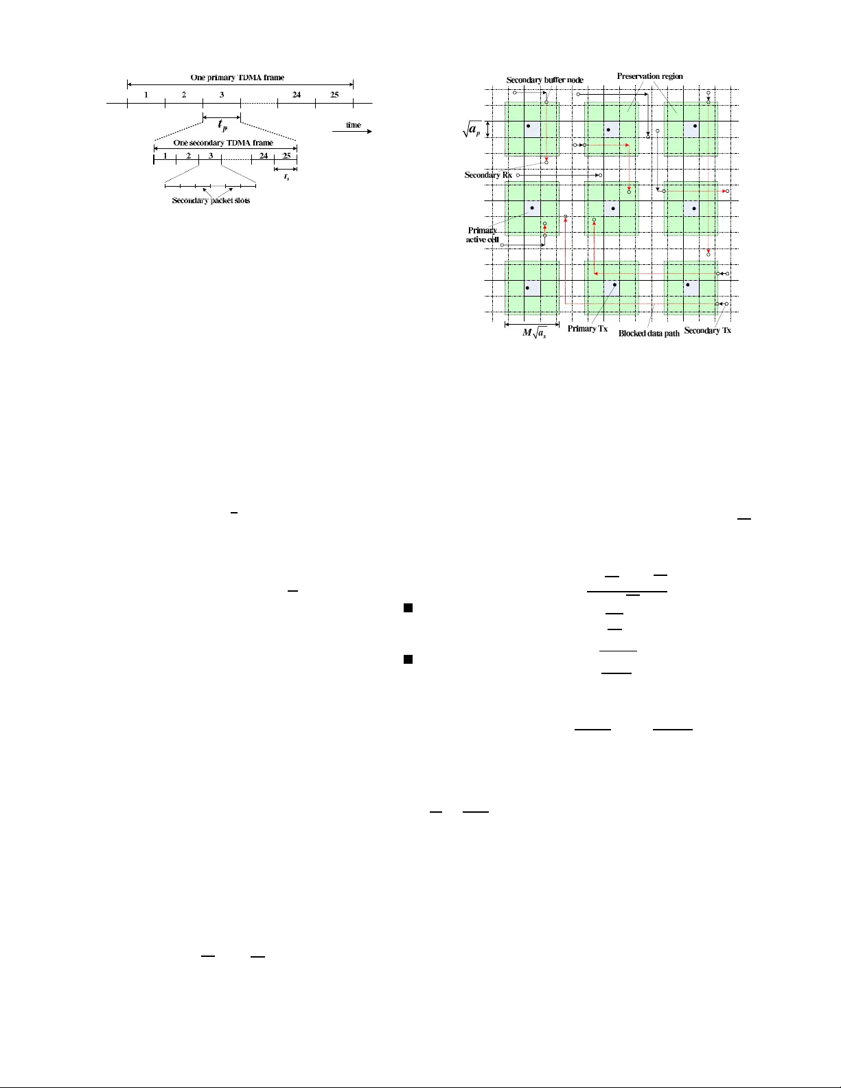
1 Scaling La ws for Overla id W ireless Networks: A Cogniti v e Radio Netw ork vs. a Primary Netw ork Changch uan Y i n, Long Gao, an d Shuguan g Cui Abstract — W e study the scaling laws for the throughputs and delays of two coexisting w ireless networks th at op erate in the same geographic region. The p rimary network consists of Poisson distributed legacy u sers of d ensity n , an d the secondary network consists of Poisso n distributed cognitiv e users of density m , with m > n . The primary users have a higher priority to access the spectrum without particular considerations fo r th e secondary users, while th e second ary users hav e to act conserva tively i n order to l imit the interference to the primary users. With a practical assumpti on that the secondary users only know the locations of the primary transmitters (not the primary receiv ers), we first show that both networks c an achiev e the same throughput scaling law as wh at Gupta and Kumar [1] established for a stand-alone wireless network if proper transmission schemes are deployed, wh ere a certain throughput is achiev able f or each individual secondary user (i.e., zero o utage) with high probability . By usin g a fl uid model, we also show th at both n etworks can achiev e the same delay-throughput tradeoff as t he optimal one established b y El Gamal et al. [2 ] f or a stand-alone wireless network. Index T erms — Ad h oc networks, overlaid wireless n etworks, throughput, del ay , cognitive radio networks. I . I N T R O D U C T I O N Initiated by th e semin al work of Gupta an d Kumar [1], the throug hput scaling law for large- scale wir eless networks has become a n active research topic [ 3]-[14]. Scaling laws p rovide a fund amental way to measure the achiev able through put of a wireless network. Con sidering n nodes that are ra ndomly distributed in a unit area and grouped indepen dently into o ne- to-one source-d estination (S-D) pairs, Gupta and Kumar [1 ] showed that typical time-slotted m ulti-hop architectu res w ith a comm on transmission range and adjacen t-neighb or com- munication can achieve a sum thro ughpu t tha t scales as Θ  p n/ lo g n  . They also showed that an alter nativ e arbi- trary network structur e with optima lly chosen traffic p atterns, node loca tions, an d transmission r anges can achieve a sum throug hput of order Θ ( √ n ) . Thus, they suggested that a factor of √ log n is the price to pay for the r andomn ess of the no de locations. In [ 3], with perco lation theor y , Fran ceschetti et al. showed that the Θ ( √ n ) sum thro ughpu t scaling is ach iev able ev en for ran domly deployed n etworks un der certain special condition s. In [4], Grossglau ser and Tse showed that by allow- ing the nod es to move independently and uniform ly , a constant throug hput scaling Θ(1) per S-D pair can be achie ved. L ater , Diggavi et al. showed that a constant throug hput per S- D p air is ac hiev able even with a o ne-dime nsional mobility The authors are with the Department of Electri cal and Computer E ngi- neering , T e xas A&M Uni versity , T X 77843, U SA (e-mail: cc yin@ieee .org, lgao@ec e.tamu.edu, cui@tamu.ed u). model [5]. In these appro aches, the n etwork area is fixed and the throug hput scales with the node density n . W e call this kind of network as d ense n etwork . On th e other hand, based on the extended network model wh ere the density o f nodes is fixed and the network area increases with n , the informa tion-theor etic scalin g laws of transp ort capacity were studied f or different values o f the pathloss expone nt α in [8]- [14]. In particular, Özg ür et a l. [ 14] p roposed a hierarch ical cooper ation scheme to achiev e a sum th rough put that scales as n 2 − α/ 2 for 2 ≤ α < 3 , i.e., asymp totically linear for α = 2 . In wireless networks, another key perf ormance m etric is delay , which incu rs the interesting problems regarding the interactions between throu ghput and d elay . The issues o f delay-thr oughp ut tradeoff for static and mobile wireless net- works hav e been ad dressed in [ 2], [15]-[21] . In [2], El Gamal et al . established the optimal delay-th rough put tradeoff for static and mobile wireless n etworks. For static netw ork s, they showed that the optimal delay-thr oughp ut tradeoff is given by D ( n ) = Θ ( nλ ( n )) , where λ ( n ) a nd D ( n ) are the throughpu t and delay per S-D p air , respectively . Using a ran dom-walk mobility mo del, they showed that a m uch high er delay of Θ ( n lo g n ) is associated with the high er thr oughp ut of Θ(1) for mobile networks. The delay -throug hput tr adeoffs in mo bile wireless networks h av e been investi gated under many other mobility models, wh ich include th e i.i. d. model [1 5], [17], [18], the hyb rid ra ndom walk m odel [ 20], and the Brownian motion mod el [ 19]. For the hierar chical coo peration scheme in a static wireless network , Özgür and Lévê que [21] sho wed that a significantly larger d elay was introduced com pared with the trad itional mu lti-hop schem e, and the delay -throu ghput tradeoff is D ( n ) = Θ  n (log n ) 2 λ ( n )  for λ ( n ) between Θ (1 / ( √ n log n )) and Θ (1 / log n ) . All the afor ementioned results focus on the through put scaling laws or th e delay- throug hput tradeoffs for a sing le wireless network. I n recent year s, the ever -growing deman d f or frequen cy r esource from wireless commu nication ind ustries imposes m ore stre ss ov er th e alr eady-cr owded r adio spe ctrum. Howe ver , a r ecent repor t by the Federal Communicatio ns Commission (FCC) Spectrum Policy T ask Force ind icated that over 90 p ercent of the licensed sp ectrum remains idle at a giv en tim e and location [ 22]. Th is m otiv ated the regulatio n bodies to consider the p ossibility of permitting secondary net- works to coexist with licensed primary networks, which is the main driving fo rce b ehind the cognitive radio tech nology [2 3]. In a secon dary network, the co gnitive users opportu nistically access the spectrum lice nsed to primary u sers accor ding to th e spectrum sen sing r esult [24], where the p rimary u sers have 2 a higher priority and the secondary users need to pr ev ent any harm ful inter ference to the primar y users [25], [26]. In this overlaid regime, the throug hput scaling law a nd th e delay-thr oughp ut trad eoff for b oth the primary and seco ndary networks are in teresting and challenging problems. Some pre- liminary work along this line appeared recen tly . In [27], [28], V u et al. con sidered the thr oughp ut scaling law f or a sing le- hop cognitive radio n etwork, where a linea r scaling law is obtained for th e secondary network with an ou tage constraint for the pr imary n etwork. In [29], Jeon et al . c onsidered a multi-hop cog nitiv e network on to p of a primary network and assumed th at the secondar y nodes kn ow the location of eac h primary nod e regardless of whether it is a transmitter (TX) o r a receiver ( RX). W ith an elegant transmission scheme, they showed that by defin ing a preservation region aro und each primary n ode, both n etworks can achieve the same th rough put scaling law as a stand-alone wire less n etwork, wh ile the secondary n etwork may suffer fr om a finite outage probab ility . In a practical co gnitive network, it is hard fo r the secondary users to kn ow the locations of prima ry receiving nodes since they may keep passi ve all the tim e. A reasonable assumption is that the seco ndary network k nows the loc ations o f the pr imary TXs. Based on th is assumption, in this paper we define a preservation region just aroun d each p rimary TX and propose correspo nding transmission scheme s for th e two n etworks. W e show that when the seco ndary n etwork h as a higher density as requested in [29], both networks can achieve the same throug hput scaling law as a stand -alone wireless network, with zero o utage f or th e seco ndary u sers with high probability . Considering a fluid model, we also show that both network s can achiev e th e same delay -throu ghput tradeo ff as the o ptimal one established for a stand-alone static wireless network in [2]. In ou r appro ach, th e primar y network d eploys a time-slotted multi-hop transm ission scheme similar to th at in [1] and does not need to c ooperate with the secondary ne twork. Note tha t, as m entioned in [29], if both the primar y n etwork an d the secondary network are willing to co operate and do time- sharing, both of th em could ea sily achie ve t he same through put scaling law as a stand-alone wireless network. The re st of the p aper is o rganized as follows. The system model, definition s, an d main results ar e d escribed in Section II. The propo sed pro tocols for the primary a nd secondar y networks are d iscussed in Section II I. The d elay and thro ugh- put scaling laws for the primary network are established in Section IV . The d elay and through put scalin g laws for the secondary network a re derived in Section V . Finally , Section VI summarizes our conclusions. I I . S Y S T E M M O D E L , D E FI N I T I O N S , A N D M A I N R E S U LT S In this section, we first describe the system mo del and assumptions about the prim ary and secondary networks, and then define the through put and delay . W e use p ( E ) to represent the probability o f event E and claim th at an event E n occurs with high pro bability ( w .h .p. ) if p ( E n ) → 1 as n → ∞ . W e use the fo llowing order notations thr ougho ut this paper . Given non-n egati ve function s f ( n ) and g ( n ) : 1) f ( n ) = O ( g ( n )) m eans that there exists a positi ve constant c 1 and an integer m 1 such that f ( n ) ≤ c 1 g ( n ) for all n ≥ m 1 . 2) f ( n ) = Ω( g ( n )) means that ther e exists a p ositiv e constant c 2 and an integer m 2 such that f ( n ) ≥ c 2 g ( n ) for all n ≥ m 2 . Namely , g ( n ) = O ( f ( n )) . 3) f ( n ) = Θ( g ( n )) me ans that both f ( n ) = O ( g ( n )) an d f ( n ) = Ω( g ( n )) hold for all n ≥ max ( m 1 , m 2 ) . A. Network Model Consider the scenario where a network of primary node s and a n etwork of second ary no des coexist over a unit squ are. The primary no des are distributed according to a Poisson po int process ( P . P . P .) of density n and random ly gro uped into one- to-one sou rce-destinatio n (S-D) p airs. Th e distribution o f the secondary nodes is following a P . P . P . of density m . The secondary n odes are also rand omly g rouped in to one- to-one S-D pairs. As the model in [2 9], we assum e that the de nsity of the secon dary network is high er than that of the pr imary network, i.e., m = n β , (1) with β > 1 . For the wireless chan nel, we only con sider the large-scale pathloss an d ign ore the effects of shad owing and small-scale multipath fading. As such, the normalized ch annel p ower gain g ( r ) is given as g ( r ) = A r α , (2) where A is a sy stem-depen dent constan t, r is the distance between the TX and the correspon ding RX, and α > 2 denotes the p athloss expon ent. In the fo llowing d iscussion, we normalize A to be unity for simplicity . The primar y network and the second ary network share the same spectrum, tim e, a nd space, while the form er one is the licensed user of th e spectrum and th us has a h igher priority to access the spectru m. The seco ndary network opportun istically access the sp ectrum while keeping its interf erence to the primary network at an “ac ceptable level”. In this paper, the “acceptable lev el” mea ns th at the presence of the secondar y network does not d egrade the throug hput scaling law of the primary network. W e assume tha t the secondar y network o nly knows the locations of the primary TXs and has no knowledge about the locations of the prim ary RXs. This is the essential difference between our model and th e model in [29], wher e the author s assumed that the seco ndary network k nows the lo cations of all the pr imary n odes. So me other aspects of our mod el ar e defined in a similar way to th at in [29], as we will d iscuss later . B. T ransmission Rate and Thr o ughpu t The ambient no ise is assumed as additive white G aussian noise (A WGN) with a n a verage p ower N 0 . During each trans- mission, we assume that each TX-RX pa ir deploys a capacity- achieving scheme, and the cha nnel bandwid th is no rmalized to 3 be un ity for simplicity . Thus the data rate of the k -th pr imary TX-RX pair is giv en by R p ( k ) = log  1 + P p ( k ) g ( k X p, tx ( k ) − X p, rx ( k ) k ) N 0 + I p ( k ) + I sp ( k )  , (3) where k · k stands for the no rm oper ation, P p ( k ) is the tr ansmit power of the k -th prim ary T X-RX pair , X p, tx ( k ) and X p, rx ( k ) are the TX an d RX location s of the k -th p rimary TX-RX pair , respectively , I p ( k ) is the sum interference from all other primary TXs to th e RX of the k -th primar y TX-RX pair, and I sp ( k ) is the sum inter ference from all the secondar y T Xs to the RX o f the k -th primary TX-RX p air . Specifically , I p ( k ) can be written as I p ( k ) = Q p X i =1 ,i 6 = k P p ( k ) g ( k X p, tx ( i ) − X p, rx ( k ) k ) , (4) where Q p is the num ber o f activ e primary TX-RX pairs, and I sp ( k ) is given by I sp ( k ) = Q s X i =1 P s ( i ) g ( k X s, tx ( i ) − X p, rx ( k ) k ) , (5) where Q s is th e nu mber o f active secondar y T X-RX pairs, P s ( i ) is the tran smit p ower of the i -th secondary TX-RX pair , and X s, tx ( i ) is the TX location of the i -th secondar y TX-RX pair . Likewise, the d ata r ate of the l - th secon dary TX-RX pair is gi ven by R s ( l ) = log  1 + P s ( l ) g ( k X s, tx ( l ) − X s, rx ( l ) k ) N 0 + I s ( l ) + I ps ( l )  , (6) where X s, rx ( l ) is the RX location of the l -th seco ndary TX- RX p air , I s ( l ) is the sum in terference fro m all oth er second ary TXs to the RX of th e l -th secondary TX-RX pair, an d I ps ( l ) is the sum in terferenc e fro m all prim ary TXs to the RX of the l -th secondary TX-RX pair . Specifically , I s ( l ) is given by I s ( l ) = Q s X i =1 ,i 6 = l P s ( i ) g ( k X s, tx ( i ) − X s, rx ( l ) k ) , (7) and I ps ( l ) is given by I ps ( l ) = Q p X i =1 P p ( i ) g ( k X p, tx ( i ) − X s, rx ( l ) k ) . (8) Now we giv e the definitions of throug hput per S-D pair and sum through put. Definition 1: The thr oug hput pe r S- D p air λ ( n t ) is d efined as the average data rate that eac h sou rce n ode can transmit to its chosen de stination w.h.p . in a multi-ho p fashion with a particular schedu ling scheme, wher e n t is the num ber of nodes in the network. W e have p  min 1 ≤ i ≤ n t / 2 lim inf t →∞ 1 t M i ( t ) ≥ λ ( n t )  → 1 , (9) as n t → ∞ , where M i ( t ) is the number of bits that S-D pair i transmitted in t time slots. Definition 2: The su m thr oug hput T ( n t ) is de fined as the produ ct between the thr oughp ut per S-D pair λ ( n t ) and th e number of S-D pairs in the network, i.e., T ( n t ) = n t 2 λ ( n t ) . (10) According to the network mod el defined in Section II.A, the number o f nodes in the prim ary network (or in the secon dary network) is a random variable. Ho wever , we will show in Lemma 1 and Lemma 3 at Section III that the number of nodes in the primary network (or in the secondary network) will be bound ed by function s of the node density w .h.p . . As such, in the following discussion, we use λ p ( n ) and λ s ( m ) to d enote the thro ughp uts p er S-D pair f or the primary network and the secondary netw ork , respectively . W e use T p ( n ) and T s ( m ) to denote the sum through puts for the prim ary network an d the secondary network, respecti vely . C. Fluid Model and Delay As in [2], we use a fluid model to study the delay -throug hput tradeoffs for the primary and secondary networks. In this model, we d ivide each time slot into mu ltiple p acket slots, and the size of the data p ackets can be scaled down to arbitrarily small with the increase of the nod e d ensity n ( or m ) in the networks. Definition 3: The delay D ( n t ) of a packet is defined as the av erage time that it takes to reach the destination no de after the departure from the source node. Let D i ( j ) denote the d elay of packet j for S-D pair i . The sample mean of delay over all packets tran smitted for S-D pair i is defined as D i = lim sup k →∞ 1 k k X j =1 D i ( j ) , (11) and the a verage delay over all S-D pairs is given by D ( n t ) = 2 n t n t / 2 X i =1 D i . The a verage delay over all realization s of the network is D ( n t ) = E h D ( n t ) i = 2 n t n t / 2 X i =1 E [ D i ] . (12) As what we d id over the notation s of thro ughp ut, in the following discussion, we use D p ( n ) and D s ( m ) to deno te the pac ket delays for the primary network and the secon dary network, respecti vely . D. Main Results The main results of this paper are as follows. 1) W e p ropose a coexistence scheme for two overlaid ad ho c wireless networks: a primary ne twork vs. a secondary network. These two n etworks o perate in the same g eograph ic region and share the same spectrum. The p rimary network has a high er priority to access the spectru m and h as no special consideration s over the 4 presence of the secondary network, while the secondar y network op erates oppo rtunistically to access the spec - trum in order to limit the in terference to th e primary network. W e assume that the pr imary ne twork uses a typical time -slotted adjacent-neighb or tra nsmission pr o- tocol (similar to that in [1]) and the secondary n etwork has a h igher density and o nly kn ows the location s of the primary TXs. By a prope rly desig ned secondar y protoco l, we show that each secondary sour ce nod e has a finite o pportu nity to transmit its packets to th e chosen destination w .h.p . , i.e., n o outage com pared with the result in [29]. 2) For the primar y network, we show that the throu ghput per S-D pair is λ p ( n ) = Θ( q 1 n log n ) w .h. p . and the sum thr oughp ut is T p ( n ) = Θ ( q n log n ) w .h. p .. These results are the same as those in a stand-alo ne ad hoc wireless network con sidered in [1]. Following the fluid mod el [ 2], we g iv e the delay -throu ghput trad eoff for the primar y network as D p ( n ) = Θ( nλ p ( n )) fo r λ p ( n ) = O ( 1 √ n log n ) , which is the o ptimal d elay- throug hput trad eoff fo r a stand-alone wireless ad hoc network established in [2]. 3) For the second ary network, we prove that the through put per S-D p air is λ s ( m ) = Θ( q 1 m log m ) w .h.p . an d the sum throu ghput is T s ( m ) = Θ( q m log m ) w .h. p .. Although due t o the presence o f the pr eservation regions, the second ary p ackets seeming ly experience larger de- lays com pared with that of the p rimary network, we show that the d elay-throu ghpu t tradeoff for th e sec- ondary network is the sam e as that in the p rimary network, i.e., D s ( m ) = Θ( mλ s ( m )) for λ s ( m ) = O ( 1 √ m log m ) . I I I . N E T W O R K P ROT O C O L S In our p roposed scheme, the pr imary network deploys a modified tim e-slotted mu lti-hop transmission scheme over th at in [1], [2], [29]. The secondary network adapts its protocol ac- cording to the pr imary tr ansmission scheme. W e first describe the prim ary proto col, then in troduce the secondar y pro tocol, and fin ally gi ve a lemma to show that with ou r pro posed protoco ls the secondary users can commu nicate witho ut o utage w .h .p. . Similarly a s in [ 29], we claim that an outage event occurs when a no de has zero opportu nity to com municate. The outag e probability is defin ed as the fractio n of node s that have zero opp ortunity to c ommun icate. A. Primary Network Pr o tocol • W e divide the un it square into small- square pr imary cells. The area of each primary cell is a p = k 1 log n n , with k 1 ≥ 1 . • W e group th e primary cells into pr imary clusters, and each cluster has K 2 p = 25 p rimary ce lls. W e split the transmission time into time d i vision mu ltiple access (TDMA) fram es, whe re each f rame h as 25 time slots that correspo nd to the n umber o f cells in each primary clu ster Fig. 1. A four-c luster example with 25 cells per cluster . T he cells in eac h cluster take turns to be acti ve along the arro wed line ov er time . with each slot of length t p . I n each time slot, one cell in each primar y cluster is chosen to b e activ e. The cells in each primar y cluster take turn s to be active in a roun d- robin fashion. All primary clu sters fo llow the same 25- TDMA transmission pattern, as sho wn in Fig. 1. • W e d efine the data p ath along which the packets traverse as the hor izontal line and then the vertical line conn ecting a sou rce and its correspo nding de stination, as shown in Fig. 2 . On e no de within a pr imary cell is d efined as a designated r elay no de, which is r esponsible fo r relay ing the packets of all the data paths passing throug h the cell. The packets will be f orwarded from cell to cell by the relay nodes first along th e horizo ntal data p ath ( HDP), then along the vertical data p ath (VDP). Nodes in a particular cell take turns to ser ve as the designated r elay node. • When a primary c ell is active, it tran smits a single packet for e ach of th e data pa ths p assing thro ugh the cell. T he transmission is also dep loyed in a TDMA fashion. The TDMA fr ame structu re fo r the primar y ne twork is shown in Fig. 3, wher e one packet slot is assigned to on e S- D d ata p ath that passes th rough or or iginates fr om a particular prim ary cell. As such , the number o f packet slots is determ ined by the total num ber of data p aths in the cell, which is based on the so-called fluid model [2 ]. The specific packet transmission proce dure is as follows: – The designated relay nod e first transmits a single packet for each o f the S-D p aths passing thro ugh the ce ll; a nd then each of the sou rce nodes with in the cell takes turns to transmit a single packet. – The r eceiving n ode mu st be located in one of the neighbo ring primary cells along the pred efined data path, unless it is a destinatio n no de, which may be located in the same ce ll. If the n ext-hop of the pa cket is the final destination , it will be directly delivered to the destination nod e; oth erwise, th e packet will b e 5 Fig. 2. Examples of HDPs and V DPs for the primary S-D pairs. Fig. 3. Structure of the primary TDMA fra me, where t p is the t ime-slot duratio n of the primary TDMA scheme. transmitted to a designated relay node. – The d esignated relay node in each primar y c ell maintains a buffer to temp orarily store the packets received from its neighborin g cells, and each p acket will be transmitted to the next hop in the next activ e time slot of the cell. • At ea ch packet slot, the TX no de transm its with p ower of P 0 a α 2 p , where P 0 is a constant. The p rimary proto col in this paper is similar to that in [2] but with different data path s and TDMA tr ansmission pattern s. As a result, we hav e the following two lemmas. Lemma 1: Let n pt denote the nu mber of total p rimary nodes in the unit square; then we hav e n 2 < n pt < en w .h.p. . Pr o of: Since n pt is a Poisson random v ariable with parameter µ = n , usin g the Ch ernoff boun d in Lemm a 11 (see Append ix), we have p  n pt ≤ n 2  ≤ e − n ( en ) n 2  n 2  n 2 =  2 e  n 2 → 0 (13) as n → ∞ , an d p ( n pt ≥ en ) ≤ e − n ( en ) en ( en ) en = e − n → 0 (14) as n → ∞ . Comb ining (13) and (14) via the union bound, we obtain p  n pt ≤ n 2 or n pt ≥ en  ≤ p  n pt ≤ n 2  + p ( n pt ≥ en ) → 0 as n → ∞ . Hen ce p  n 2 < n pt < en  = 1 − p  n pt ≤ n 2 or n pt ≥ en  → 1 as n → ∞ , wh ich completes the proof. Lemma 2: For k 1 ≥ 1 , eac h primary c ell contain s at least one but no mo re than k 1 e log n primary nodes w . h.p. . Pr o of: Let n p denote the n umber of prim ary n odes in a particular primar y cell; then n p is a Poisson r andom variable with parameter µ = na p = k 1 log n . The pr obability of n p = 0 is gi ven by p ( n p = 0) = e − k 1 log n ( k 1 log n ) k k !     k =0 = 1 n k 1 . (15) By the union boun d, the pr obability that at least one primary cell having no nodes is up per-bounded by th e total num ber of cells multiplied by p ( n p = 0) , which is p ( At least o ne primary cell has no nodes ) ≤ 1 a p p ( n p = 0) = 1 k 1 n k 1 − 1 log n → 0 as n → ∞ fo r k 1 ≥ 1 . Now consider the upper bound of n p . By the Cher noff bound in Lemma 11 (see Appendix ), we have p ( n p ≥ k 1 e log n ) ≤ e − k 1 log n ( ek 1 log n ) k 1 e log n ( k 1 e log n ) k 1 e log n = n − k 1 . As long as k 1 ≥ 1 , by th e union bound, we ha ve p ( At least one primar y cell has more tha n k 1 e log n nodes ) ≤ 1 a p n − k 1 = 1 k 1 n k 1 − 1 log n → 0 as n → ∞ . Th is completes the proof. B. Second ary Network Pr otoco l • W e divide the unit area in to square secondary cells with size a s = k 2 log m m , with k 2 ≥ 1 . • W e g roup the second ary c ells into second ary clusters. Each secondary cluster has K 2 s = 25 cells. Similar to the primary network proto col, the secondary network also follows a 25-T DMA p attern to communicate. W e let the duration o f each second ary TDMA frame eq ual to that of one p rimary time slot. T he relation ship between the primary TDMA frame and the seco ndary TDMA f rame is sh own in Fig. 4, where each secon dary time slot is further divided into packet slots. • T o limit the interferen ce fro m the second ary n odes to the primary nodes, we defin e a p reservation region as a square co ntaining M 2 secondary cells around a particu lar primary c ell in which an ac ti ve primary TX (not the RX) is loca ted, where M is an integer and the v alue will be defined later . No second ary nodes in the preservation regions are allowed to transmit. • The de signated relay n odes and data p aths fo r the sec- ondary network are d efined in the same way as those for the pr imary network. As shown in Fig. 5 , when a particular seco ndary cell outside the pr eservation region 6 Fig. 4. Structure of the secondary TDMA frame and its relati onship with the primary TDMA frame, where t s is the time-slot duration for the sec ondary TDMA scheme. is acti ve, its designated r elay node transmits a single packet for each of the data paths passing through the cell, and e ach of th e second ary sour ce nod es within the cell takes turn s to transmit a sing le packet. The packet is transmitted to the next-hop relay node or the destination node in neighb oring secondary cells along the HDP o r VDP path. Note that if the RX n ode is the destination node, it may b e located in the same cell, as we discussed for the primary protocol. • When a seco ndary cell falls i nto a preservation region 1 , its designated relay node buffers th e packets th at it receives; it waits until the preservation region is clear ed and the cell is acti ve to deliv er the packets to the n ext hop. • At each packet slot, the active secondar y TX node tran s- mits with power of P 1 a α 2 s , where P 1 is a constant. Similarly as in the pr imary network case, we h av e th e following two lemma s for the seco ndary network. Lemma 3: Let n st denote the to tal number of secondary nodes in the un it square; then we have m 2 < n st < em w .h. p. . Pr o of: The proof is similar to that of Lemma 1. Lemma 4: For k 2 ≥ 1 , eac h secon dary cell conta ins at least one but no more than k 2 e log m secondary nodes w .h. p. . Pr o of: The proof is similar to that of Lemma 2. Regarding the cluster size, note th at the value of K s is not necessarily the same as th at of K p . Here we c hoose K s = K p for simplicity . W ithou t loss of generality , we also choose k 1 = k 2 in the following discu ssion. Now , let us discuss how to ch oose th e value of M , i. e., the size for the preservation region. Con sidering the fact that the primary TX may only tran smit to a n ode in its adjacent cells or within the same cell, the preser vation region should accommo date at least 9 pr imary cells to prote ct the potential primary RX. Since the p rimary RX may b e located close to the outer bound ary of the 9-cell region , we shou ld add another layer of protec ti ve seco ndary cells. As such, any activ e secon dary TXs outside the pr eservation region are at least certain-distance- away from the p otential p rimary RX. Therefo re, we define the side length o f th e pre servation square region as M √ a s ≥ 3 √ a p + 2 ǫ p , (16) 1 Note that the secondary nodes located in the preserv ation regi ons can still recei ve pack ets from TXs outside the preserva tion regio ns, althoug h the y are not permitted to transmit packets. Fig. 5. Preservat ion region and examples of secondary data paths. where ǫ p > 0 defines th e width of th e pr otective second ary strip aroun d th e 9 primary cells in the preservation region . There is a tra deoff in choosin g th e value of ǫ p . If we ch oose a larger ǫ p , the interf erence from the seco ndary network to the p rimary network will be less. Howev er, the opp ortunity for the seco ndary network to access the spectrum will also be less since the un preserved area in the u nit square will be reduced . In the following discussion, we set ǫ p = √ a s for simplicity . Accord ingly , the minim um value of M can b e set as M = ⌊ 3 √ a p + 2 √ a s √ a s ⌋ = ⌊ 3 r a p a s ⌋ + 2 ≈ 3 s n β − 1 β , (17) where ⌊·⌋ denotes the flooring operation . In the last equation of (17), we applied a p = k 1 log n n , a s = k 2 log m m , k 1 = k 2 , and (1), assuming that n is large eno ugh. In the follo wing discussion, “ n is large” o r “ n is large en ough” means that, for a fixed β , n is chosen to satisfy a s ≪ a p . For e xamp le, when k 1 = k 2 , β = 2 , n = 1000 , we h av e m = 10 00000 and a p a s = n β − 1 β = 500 . Note that the preservation region defined here is larger than that in [29] due to the fact that we o nly know the locatio ns of primary TXs. I f a second ary n ode falls inside a preservation region, it will be silenced . If no t, it may beco me acti ve and has an opp ortunity to transmit its packets. Acco rdingly , we call the unpreser ved r egion as the “active region”. Since the locatio ns of pre servation region s chan ge periodica lly ac cording to the activ e time slots in the primary T DMA f rame, f rom th e po int view of a specific seco ndary nod e, it is per iodically located in the activ e r egion. W e define the following termin ology to measure the fr action of time in which a secondar y cell is located in the activ e region. 7 Fig. 6. Preservat ion regions and worst place s in one primary cluster . Definition 4: The opp ortunistic factor of a second ary cell is defined as the f raction of time in which it is located in the activ e region. W e use th e following lemm a to sho w th at, with the p rotocols defined previously , each ind i vidu al secondary source node has a finite o pportun ity to transmit its p ackets to the cho sen destination w .h. p. . Lemma 5: W ith the proposed transm ission protoco l, we have the following results: 1) The op portunistic facto r for a second ary cell is 9 25 ≤ η ≤ 16 25 , for n is large enough. 2) Each in dividual secon dary node h as a finite opportun ity to transmit its p ackets to the chosen destination, i.e., zero outage, w .h .p. . Pr o of: Consider o ne pr imary cluster of 25 p rimary cells as shown in Fig. 6, wher e the pr eservation regions ar e illustrated as the shad ed area when the upper-left primary c ell is a cti ve in this and ne ighborin g clusters. The primary ce lls will take turns to be activ e over time (see Fig. 1) an d the locations of the p reservation regions will chan ge accordingly . W e can easily verify that any po int in the cluster has a finite oppor tunity to be in the ac ti ve region wh en n is large. Howe ver , during each period of a prim ary TDMA fr ame, the fractio ns of time for different seco ndary nodes to be in the active r egion are no t the sam e. T he worst plac es are the squares with side le ngth of 2 √ a s around the vertices of each primary cell, as shown by those dee ply-shade d small s quar es in Fig. 6. Th e op portun istic factor o f the seconda ry ce lls in these squares is 9 25 . The b est places are the squares with side len gth of √ a p − 2 √ a s inside each primary cell, as shown by th e deeply-sh aded squares in Fig. 7. The o pportu nistic factor of the secondary cells in these squar es are 16 25 . When the seco ndary cell lies in other places, the oppo rtunistic factor is b etween 9 25 and 16 25 . The condition that a secondary n ode is located in the active region is not sufficient to ensure th at it can transmit p ackets Fig. 7. The best places in one primary cluster . to the destina tion alon g the p redefined data path . Recall tha t the secondar y n etwork also de ploys a TDMA scheme with adjacent-n eighbor transmission. The sufficient condition to ensure that eac h indi vidu al secondar y n ode h as a finite ch ance to transmit p ackets is that the seco ndary cell in w hich the n ode is located will be assigned with at least one active second ary TDMA slot within each second ary fr ame, wh enever the cell is in the activ e region. Since in each pr imary time slot, we have on e comp lete seconda ry TDMA frame in ou r pro tocol, the above sufficient condition is indeed satisfied. Based on the ab ove discussions, during each period of a primar y TDMA frame, each second ary cell has a finite oppor tunity to be located in the active region with an op- portun istic factor of 9 25 ≤ η ≤ 16 25 , and eac h of them is assigned with a seco ndary TDMA slot. Ac cording to the secondary pro tocol, wh en a second ary cell is active, each packet buffered in this cell will be assigne d with a packet slot w . h.p . to be transmitted, sin ce the total num ber of data paths that pass thr ough or originate fro m each seco ndary cell is upper-bound ed w .h.p . (see Lemma 10 in Section V). Thus, the pac kets from any seco ndary so urce nod e have a finite oppor tunity to b e transmitted along the pre defined data path to the ch osen destination w .h.p. . This completes the pro of fo r the zero outage proper ty . There is a significant difference between our result here and that in [29]. The authors in [29] defin ed preservation regions o f 9 secondary cells aro und e ach primary node, and the positions of the pr eservation regions are fixed. If the secondary nodes are located in th e preservation regions, the y will never be active. The refore, the seco ndary network in [ 29] usually suffers from a non -zero outag e pr obability , even thoug h the outage prob ability is upper-boun ded w .h .p. . In o ur case, each secondary node has a finite opportunity to be active such that we have zero outage w .h.p. . 8 I V . D E L A Y A N D T H RO U G H P U T A N A L Y S I S F O R T H E P R I M A RY N E T W O R K In this section, we discuss the delay a nd through put scalin g laws as well as the delay-th rough put tradeoff fo r the primary network. The main results are given in three theorems. W e fir st present the delay and throug hput scaling laws, th en establish the delay-th rough put tra deoff fo r the primary network. A. Delay Analysis for the Primary Network The p acket delay for th e p rimary network is given by th e following th eorem. Theor em 1: Accord ing to th e prim ary network pr otocol in Section III, the packet delay is gi ven by D p ( n ) = Θ 1 p a p ( n ) ! , w.h.p.. (18) Pr o of: W e first derive the av erage numb er of ho ps for each pa cket to tra verse along the pr imary S-D data path, then use the fact that the time for each primary pac ket to spend at each hop is a con stant, 25 t p , as shown in Fig. 3 , and fin ally calculate the av erag e d elay for each primary S-D pair . Since each pr imary hop spans a d istance o f Θ  p a p ( n )  w .h .p. , the numb er of hops fo r a primary p acket along the S-D data path i is Θ  d p ( i ) √ a p ( i )  w .h .p. , w here d p ( i ) is the length of the primary S-D data path i . Hence, the number o f h ops trav ersed by a primary packet, a veraged over all S-D p airs, is Θ  2 n pt P n pt / 2 i =1 d p ( i ) √ a p ( n )  w .h .p .. The d ata path length d p ( i ) is a random variable, with a maximum value o f 2. According to th e law of large number s, as n pt → ∞ , the av erag e distance between primary S-D pair s is 2 n pt n pt / 2 X i =1 d p ( i ) = Θ (1) . Therefo re, the a verage num ber of hops for a prima ry packet to traverse is Θ  1 √ a p ( n )  w .h .p. . Since we u se a fluid model such that th e packet size of the prim ary network scales propo rtionally to the th rough put λ p ( n ) , each packet arrived at a primary cell will be transmitted in the next acti ve time slot of the cell. As such, the maximum time spent at each prim ary hop fo r a particu lar packet is 25 t p . Hence, the average delay for each primary packet is gi ven b y D p ( n ) = Θ 25 t p p a p ( n ) ! = Θ 1 p a p ( n ) ! , w.h.p, (19) which completes the proof. The above p roof fo llows the same logic as the proof o f Theorem 4 in [2]. The tw o differences are th at we use HDPs and VDPs as the packet ro uting paths instead of th e direct S-D links and we use a different TDMA transmission pattern . B. Thr oughpu t Analysis for the Primary Network For the prima ry ne twork, the throu ghput per S-D pair an d the sum th roughp ut scaling laws a re given in the following theorem. Theor em 2: W ith the prima ry protoco l defined in Section III, the primary network can ach ie ve the f ollowing th rough put per S-D pair and sum throughp ut w .h.p . : λ p ( n ) = Θ  r 1 n log n  (20) and T p ( n ) = Θ  r n log n  . (21) Before we g iv e the p roof of the above th eorem, we first give two lemm as, then use th ese lem mas to prove th e th eorem. The ma in logical flo ws in the proof s of these lemmas and the theorem are motiv ated by th at in [29] and [15]. Lemma 6: W ith the primary pro tocol defin ed in Section I II, each TX no de in a primar y cell can suppo rt a c onstant data rate of K 1 , where K 1 > 0 is indepen dent o f n . Pr o of: In a gi ven primary packet slot, supp ose we h av e Q p activ e primary cells and Q s activ e secon dary ce lls. T he data rate suppo rted f or a TX no de in the i -th active prim ary cell can be calculated as follows: R p ( i ) = 1 25 log  1 + P p ( i ) g ( k X p, tx ( i ) − X p, rx ( i ) k ) N 0 + I p ( i ) + I sp ( i )  , (22) where 1 25 denotes the rate loss due to the 25-TDMA transmis- sion in th e p rimary network. No te th at since th ere is only one activ e primar y link in itiated in each pr imary cell at a giv en time, we index the activ e link initiated in th e i -th active primary cell as th e i - th active primary link in the whole network. I n Fig. 8, we sh ow the primary interference sources to the pr imary RX o f th e i -th active primary link, where the shaded ce lls re present the active p rimary cells based on the 25-TDMA p rotocol. From th e fig ure, w e see tha t we h av e 8 primary interferer s with a distance of at least 3 √ a p , 16 primary interfer ers with a distance of at lea st 7 √ a p , and so on. Thus, I p ( i ) is upper-bou nded as I p ( i ) = Q p X k =1 ,k 6 = i P p ( k ) g ( k X p, tx ( k ) − X p, rx ( i ) k ) < P 0 ∞ X t =1 8 t (4 t − 1) − α = I p < ∞ , (23) where we used the relation ship th at P p ( k ) = P 0 a α 2 p for all k ’ s and the fact that the series P ∞ t =1 8 t (4 t − 1) − α conv erges to a con stant f or α > 2 (see Lemma 12 in Append ix). Du e to the preservation region s, a minimum distance √ a s can be guara nteed from all secon dary activ e TXs to any active 9 primary RXs. Thus, I sp ( i ) is upper-bou nded as I sp ( i ) = Q s X k =1 P s ( k ) g ( k X s, tx ( k ) − X p, rx ( k ) k ) + P 1 a α 2 s ( √ a s ) − α < P 1 ∞ X t =1 8 t (4 t − 1) − α + P 1 = I sp < ∞ , (24) where we u sed th e fact that P s ( k ) = P 1 a α 2 s for all k ’ s a nd Lemma 12. Therefo re, we have R p ( i ) > 1 25 log 1 + P 0 ( √ 5) − α N 0 + I p + I sp ! = K 1 > 0 , (25) where the relationship that k X p, tx ( i ) − X p, rx ( i ) k ≤ p 5 a p is used (see Fig. 8). This completes the proof. Lemma 7: For a p ( n ) = k 1 log n/n , the number o f p rimary S-D paths (including b oth HDPs and V DPs) that p ass through or originate from each primary cell is O  n p a p ( n )  w .h .p. . Pr o of: See the p roof of Lemma 3 in [29] o r the proof of Lemma 2 in [15]. Now we give th e proof for Theorem 2. Pr o of: Consider the proo f of the per-node thro ughp ut in ( 20). Acc ording to th e d efinitions in Sectio n I I, we need to show that there are dete rministic con stants c 2 > 0 and c 1 < + ∞ to satisfy lim n →∞ p  c 2 √ n log n ≤ λ p ( n ) ≤ c 1 √ n log n  = 1 . (26) A loose u pper boun d of the p er-node th rough put for the primary n etwork is achieved when the seconda ry network is absent. Gu pta and Kumar [1] have already showed that such an upp er b ound given in (26 ) exists. W e th en only n eed to consider the proof for the lower bo und. Since a given TX node in each prim ary cell can suppor t a constant data rate of K 1 (see Lemma 6), eac h primary S -D pair can a chieve a data rate o f at least K 1 divided by the m aximum number of data paths that pass through and originate from the primary cell. From Lemma 7, we know that the number of data path s that pass throug h or originate from each primar y cell is O  n p a p ( n )  w .h .p.. Therefo re, th e th rough put per S- D pair λ p ( n ) is lower-bounded by Ω  1 n √ a p ( n )  w .h .p. , i.e., the lower b ound is Ω  1 √ n log n  w.h.p. . From Lemma 1 , the nu mber of pr imary S-D pairs is lo wer- bound ed by n 4 w .h .p. . Thus, th e sum through put S p ( n ) is lower -boun ded by n 4 λ p ( n ) w .h.p . , i.e., the lo wer bo und is Ω  q n log n  w .h .p. . The up per boun d of S p ( n ) is already established in [1]. This completes the proof. From th e proof of Theor em 2 , th e th rough put per S-D p air fo r the primary network can be written as λ p ( n ) = Θ 1 n p a p ( n ) ! , w .h.p.. (27) Fig. 8. Int erference from the concurrent primary transmissions to the worst- case primary RX of the transmission from the i -th primary cell. C. Delay-thr oughp ut T radeo ff for the Primary Network Combining the results in (1 8) and (27), th e delay-thro ughpu t tradeoff fo r the primary network is giv en b y the following theorem. Theor em 3: W ith the prima ry protoco l defined in Section III, the delay-thro ughpu t tr adeoff is D p ( n ) = Θ ( nλ p ( n )) , f or λ p ( n ) = O  1 √ n log n  . (2 8) V . D E L A Y A N D T H RO U G H P U T A N A L Y S I S F O R T H E S E C O N DA RY N E T W O R K The dif fere nce between the primary a nd the seco ndary trans- mission schemes arises from the presence of th e preservation regions. When their pa ths ar e blocked by the preservation regions, th e secondary relay nodes buf fer the packets and wait until the next hop is a vailable. Due to the p resence of the preservation region , the seco ndary packets will experienc e a larger d elay com pared with the primary p ackets. H owe ver , the av erage packet delay per hop fo r each seco ndary S-D data path is still a constant as we discussed la ter . Thus, we can show that th e thro ughpu t scaling law and th e delay -throu ghput tradeoff for the seco ndary network are the same as tho se in the primary network. I n the fo llowing discu ssion, we first analyz e the average packet delay , then discu ss the throu ghput scaling law , and finally describe the delay-throug hput tradeoff. A. Delay Analysis for the Seconda ry Network The av erag e packet delay fo r the secondary network is gi ven by the following theo rem. Theor em 4: Accord ing to the proposed secondary network protoco l in Section III, the packet delay is given by D s ( m ) = Θ 1 p a s ( m ) ! , w .h.p.. (29) 10 Before giving the proof of The orem 4, we present the following lem ma. Lemma 8: The a verage p acket delay for each secon dary h op is Θ(1) . Pr o of: Let D j s,h ( i ) deno te the p acket delay for the secondary network over h op j and S-D pair i . As shown in Fig. 4 , if there ar e no preservation regions, each secondar y cell h as o ne active time slot in each primary time slot. In another word , each secondar y packet will exper ience a worst- case delay of t p at each hop, i.e., D j s,h ( i ) = t p . When we have the preservation regions, accord ing to Lemm a 5 , D j s,h ( i ) is a bou nded rando m variable. I t dep ends on the locatio n of the active TX fro m wh ich the seco ndary pa cket dep arts. As shown in Fig. 4 and Fig. 6, wh en the ac ti ve TX is located in the worst places a s shown in Fig. 6, D j s,h ( i ) is 1 η min t p , where η min = 9 25 is the minim um value of the oppo rtunistic factor η . Similarly , when th e active TX is located in the best places as shown in Fig. 7, D j s,h ( i ) is 1 η max t p , where η max = 16 25 is the m aximum value of the opp ortunistic factor η . Hence, the ensemb le average of D j s,h ( i ) will be a co nstant c 0 , where 1 η max t p < c 0 < 1 η min t p , i.e., E h D j s,h ( i ) i = Θ(1) . This completes the proof. Now , let us prove Theorem 4. Pr o of: Sinc e eac h second ary hop covers a distance of Θ  p a s ( m )  w .h .p ., and similarly as in the pro of of Theorem 2, the average leng th of eac h secon dary S-D data path is Θ(1) , the a verage number of hop s fo r each second ary packet is Θ  1 √ a s ( m )  w .h .p .. From Lemm a 8, the average packet delay for ea ch second ary hop is Θ(1) . Th erefore , the av erage packet delay for the secondary network is D s ( m ) = Θ 1 p a s ( m ) ! w .h .p ., which completes the proof. B. Thr oughpu t Analysis for the Secon dary Network For the seco ndary network, th e throug hput scaling law is giv en by the following th eorem. Theor em 5: W ith the secondary pro tocol define d in Section III, the secon dary network ca n achieve the f ollowing th rough - put per-node and sum th rough put w .h.p. : λ s ( m ) = Θ  r 1 m log m  (30) and T s ( m ) = Θ  r m log m  . (31) Similarly as in the p rimary network case, we first present two lemmas, then use these lemmas to prove Theorem 5. Lemma 9: W ith the proposed second ary protocol, each TX node in a secon dary cell can suppor t a da ta rate of K 2 , where K 2 > 0 is indepen dent o f m . Pr o of: Due to the presence of the preservation regions, a minimum distance of 1 . 5 √ a p from all p rimary T Xs to a specific active secon dary RX can be gua ranteed. At a g iv en secondary packet slot and at the i -th secon dary link (i.e., the activ e transmission initiated in the i - th secondar y cell), the interferen ce from all a cti ve primary TXs is upper-bound ed as I ps ( i ) < P 0 a α 2 p ∞ X t =1 8 t ((3 t − 1) √ a p ) − α + P 0 a α 2 p  1 . 5 √ a p  − α < P 0 ∞ X t =1 8 t (3 t − 1) − α + P 0 (1 . 5) − α = I ps < ∞ , (32) where we ap plied the same techniq ue as in the proo f of Lemma 6 to ob tain the u pper bound. Likewise, I s ( i ) is upper- bound ed b y I s = P 1 P ∞ t =1 8 t (4 t − 1) − α , which conv erges to a con stant a s shown in Lemma 12 (see the Ap pendix ). Considering th e effects of the pr eservation region, the lower bound of th e d ata rate that is supported in each second ary cell can be written as R s ( i ) > 1 25 η min log 1 + P 0 ( √ 5) − α N 0 + I ps + I s ! = K 2 > 0 , (33) where η min = 9 25 represents the penalty d ue to the presence of the preservation region. Thu s, we can gu arantee a constant data rate K 2 > 0 fo r a given TX node in each secondary cell, which completes the proof. Lemma 10: For a s ( m ) = k 2 log m/m , the num ber of secondary S-D paths ( including both HDPs and VDPs) that pass thro ugh or originate from each seco ndary cell is O  m p a s ( m )  w .h .p. . Pr o of: T he pr oof of Le mma 1 0 follows the same log ic as that in the proof of Lemma 7. Now , let us prove Th eorem 5. Pr o of: The proo f of Theore m 5 is similar to th e pro of of Theorem 2. Similarly as in The orem 2, the th roughp ut per S-D pair o f the secondary network can b e written as λ s ( m ) = Θ 1 m p a s ( m ) ! , w .h.p.. (34) C. Delay-thr oughp ut T radeo ff for the Seco ndary Network Combining the results in (2 9) and (34), th e delay-thro ughpu t tradeoff for the secondar y network is given by the fo llowing theorem. Theor em 6: W ith the secondary pro tocol define d in Section III, the d elay-thro ughpu t tradeoff for th e second ary network is D s ( m ) = Θ ( mλ s ( m )) , f or λ s ( m ) = O  1 √ m log m  . (35) V I . C O N C L U S I O N In this pap er , we studied the co existence o f two wireless networks with different priorities, wh ere the p rimary network has a h igher priority to ac cess th e spectrum, and the seco ndary network op portun istically explore the spectr um. When the 11 secondary network has a higher density , with ou r p roposed protoco ls, both of these networks can achieve the throu ghput scaling law pr omised by Gup ta and Kumar in [1]. Comparing with the recent re sult in [29], we only assum ed the knowledge about the p rimary TX locations and ther e is no o utage penalty for the secon dary nodes. By using a fluid model, we also showed that both networks can achieve the same delay- throug hput trad eoff as the o ptimal o ne established for a stand- alone wireless network in [2]. A P P E N D I X In the appendix, we first recall the usefu l Chernoff bound f or a Poisson r andom variable from [3 0]; then we g iv e a lemma to show that th e infinite series sums in Lemma 6 and Lemma 9 conv erge to a constan t. Lemma 11: (Theorem 5.4 in [30]) Let X be a Poisson random variable with p arameter µ . 1) If x > µ , the n p ( X ≥ x ) ≤ e − µ ( eµ ) x x x ; 2) If x < µ , the n p ( X ≤ x ) ≤ e − µ ( eµ ) x x x . Lemma 12: The sum P ∞ t =1 at ( bt − 1) − α conv erges to a constant, where α > 2 , a and b are positi ve in tegers. Pr o of: ∞ X t =1 at ( bt − 1) α = a b α ∞ X t =1 t ( t − 1 b ) α = a b α ∞ X t =1 1 ( t − 1 b ) α − 1 + a b α +1 ∞ X t =1 1 ( t − 1 b ) α . (36) Applying the following ineq uality ∞ X t =1 1 ( t − 1 b ) α ≤ 1 (1 − 1 b ) α +  ∞ 1 1 ( t − 1 b ) α dt to (36), we obtain ∞ X t =1 at ( bt − 1) α ≤ a b α  1 (1 − 1 b ) α − 1 +  ∞ 1 1 ( t − 1 b ) α − 1 dt  + a b α +1  1 (1 − 1 b ) α +  ∞ 1 1 ( t − 1 b ) α dt  = a b α  1 − 1 b  α − 1 + a  1 − 1 b  − α +2 b α ( α − 2) + a b α +1  1 − 1 b  α + a  1 − 1 b  − α +1 b α +1 ( α − 1) , where the last e quation is a con stant wh en α > 2 . This completes the proof. A C K N OW L E D G M E N T The au thors would like to thank Dr . T ie Liu for h elpful discussions during the course of this work. R E F E R E N C E S [1] P . Gupta and P . R. Kumar , “The capa city of wireless networks, ” IE EE T rans. Inf . Theory , vol. 46, no. 2, pp. 388-404, Mar . 2000. [2] A. El Gamal, J. Mamm en, B. Prabhakar , and D. Shah, “Optimal throughput -delay scalin g in wireless networks—P art I: The fluid model, ” IEEE T rans. Inf. Theory , v ol. 52, no. 6, pp. 2568-2592, Jun. 2006. [3] M. Franceschet ti, O. Dousse, D. Tse, and P . Thiran, “Clo sing the gap in the capa city of wireless networks via percol ation theory , ” IEE E T rans. Inf. Theory , vol. 53, no. 3, pp. 1009-101 8, Mar . 2007. [4] M. Grossglauser and D. N. C. Tse, “Mobilty increases the capacity of ad-hoc wirel ess networks, ” IEE E/ACM T rans. Net w ., vol. 10, no. 4, pp. 477-486, Aug. 2002. [5] S. N. Digga vi, M. Grosslauser , and D. N. C. Tse, “Even one- dimensional mobility increases ad hoc wireless ca pacity , ” IEEE T rans. Inf. Theory , vol. 51, no. 11, pp. 3947-3954 , Nov . 2005. [6] F . Xue and P . R. Kumar , Scaling Laws for A d Hoc W irel ess Networks: An Information Theoreti c Appr oach . Now Publishers, T he Netherla nds, 2006. [7] S. R. Ku llkarni and P . V iswanath, “ A dete rministic approach to through - put scaling in wireless network s, ” IEEE T rans. Inform. Theory , vol. 50, no. 6, pp. 1041-1049, Jun. 2004. [8] L. -L. Xie and P . R. Kumar , “ A network information theory for wireless communicat ion: Sca ling laws and optimal operation, ” IEEE T rans. Inf . Theory , vol. 50, no. 5, pp. 748-767, Feb . 2004. [9] L. -L. Xie and P . R. Kumar , “On the path-loss attenuati on re gime for positi ve cost and linear scaling of transport capacit y in wireless netw orks, ” IEEE Tr ans. Inf. Theory , vol. 52, no. 6, pp. 2318-2328, Jun. 2006. [10] A. Jovicic , P . V iswanath, and S. R. Kulka rni, “Upper bounds to transpor t capac ity of wireless netw orks, ” IEEE T rans. Inf . Theory , v ol. 50, no. 11, pp. 2555-2565, Nov . 2004. [11] S. Ahmad, A. Jovicic, and P . V iswanat h, “Outer bound s to the capacity regi on of wireless net works, ” IEEE T rans. Inf. Theory , v ol. 52, no. 6, pp. 2770-2776, Jun. 2006. [12] F . Xue and P . R. Kumar , “The transport capacity of wirele ss netw orks under f ading chann els, ” IE EE T rans. Inf . T heory , vol. 51, no. 3, pp. 834- 847, Mar . 2005. [13] O. Lévê que and ˙ I. E . T elatar , “Information- theoretic upper bounds on the capacity of lar ge exten ded ad hoc wireless networks, ” IE EE T rans. Inform. Theory , vol . 51, no. 3, pp. 858-865, Mar . 2005. [14] A. Özgür , O. L évêque , and D. N. C. T se, “Hierarchica l cooperat ion achie ves opti mal capaci ty scaling in ad hoc networ ks, ” IEEE T rans. Inf. Theory , vol. 53, no. 10, pp. 3549-3572, Oct. 2007. [15] S. T oumpis and A. J. Goldsmith , “Lar ge wirel ess netw orks under fading, mobility , and delay constraints, ” in Pr oc. IEEE INFOCOM , Hong Kon g, Mar . 2004. [16] A. El Gamal, J. Mammen, B. Prabhakar , and D. Shah, “Opti mal throughput -delay scaling in wireless networks—Pa rt II: Constant-size pack ets, ” IE EE T rans. Inf. Theory , vol. 52, no. 11, pp. 5111-5116, Jun. 2006. [17] M. J. Neely and E. Modian o, “Capa city and del ay tradeof fs for ad hoc mobile netw orks, ” IEEE T rans. Inf. Theory , vol . 51, no. 6, pp. 1917- 1937, Jun. 2005. [18] X. Lin and N. B. Shrof f, “The fund amental ca pacity-de lay tradeof f in larg e mobile ad hoc netwo rks, ” in Third Annual Mediterr anean Ad Hoc Network ing W orkshop , Bodrum, T urke y , Jun. 2004. [19] X. Lin, G. Sharma, R. Maz umdar , and N. B. Shrof f, “Dege nerate delay- capac ity tra de-of fs in ad hoc networks with Brown ian mobility , ” IEEE T rans. Inf . Theory , vol . 52, no. 6, pp. 2777-2784, Jun. 2006. [20] G. Sharma, R. Mazumdar , and N. B. Shrof f, “Delay and capacit y trade - of fs in mobile ad hoc n etworks: A globa l perspecti ve, ” IEE E/ACM T rans. Netw ., vol. 15, no. 5, pp. 981-992, Oct. 2007. [21] A. Özgür and O. L évêque, “Throughput-dela y trade-of f for hierarchic al coopera tion in ad hoc wireless networks, ” Preprint. Jan. 2008. [Online]. A vai lable: http:/ /arxi v .org/p df/0802.2013v1. [22] Federal Communications Commission, Spectrum Policy T ask Force, Rep. ET D ock et no. 02-135, Nov . 2002. [23] S. Haykin, “Cogniti ve radio: Brain-empo wered wireless communica- tions, ” IEE E J. Sel. Areas Commun. , vol. 23, no. 2, pp. 201-220, Feb . 2005. 12 [24] Z. Quan, S. Cui, and A. Sayed, “Optimal linear cooperatio n for spectrum sensing in cogniti ve radio networks, ” IEEE J . Sel. T opics Signa l P r ocess. , vol. 2, no. 1, pp. 28-40, Feb . 2008. [25] A. Sahai, N. Hoven, S. M. Mishra, and R. T andra, “Fundament al tradeof fs in robu st s pectrum sensing for opportunistic frequenc y reuse, ” T ech. Rep., Mar . 200 6. [Online]. A vaila ble: http:/ /www .eecs.berk eley . edu/~sahai/Papers/C ognitiveT e chReport06.pdf. [26] N. Hove n and A. Sahai, “Power scaling for cogniti ve radio, ” in Int’l Conf . on W ire less Networks, Comm. and Mobile Computing , vol. 1, pp. 250-255, Jun. 2005. [27] M. V u, N. De vroye , M. Sharif, and V . T arokh, “Scaling laws of cogniti ve netw orks, ” in P r oceedi ngs of Crown Com , Aug. 2007. [28] M. V u and V . T arokh, “Scaling laws of single- hop cogniti ve netw orks, ” Preprint. [Online]. A vai lable: http:/ /people.seas.ha rvard.edu/~mai vu/cognet_scaling.pdf. [29] S. -W . Jeon, N. Devro ye, M. V u, S. -Y . Chung, and V . T arokh, “Cogni- ti ve networks achie ve thr oughput scali ng of a homogeneous network, ” Preprint. Jan. 2008. [Online]. A v ailable : ht tp://arxi v .org/pdf/0 801.0938. [30] M. Mitzenmache r and E. Upf al, Pr obabilit y and Comput ing: Ran- domized Algorithms and Pr obabili stic Analysis , Cambridge , U. K.: Cambridge Univ . Press, 2005.