Pruning Attribute Values From Data Cubes with Diamond Dicing

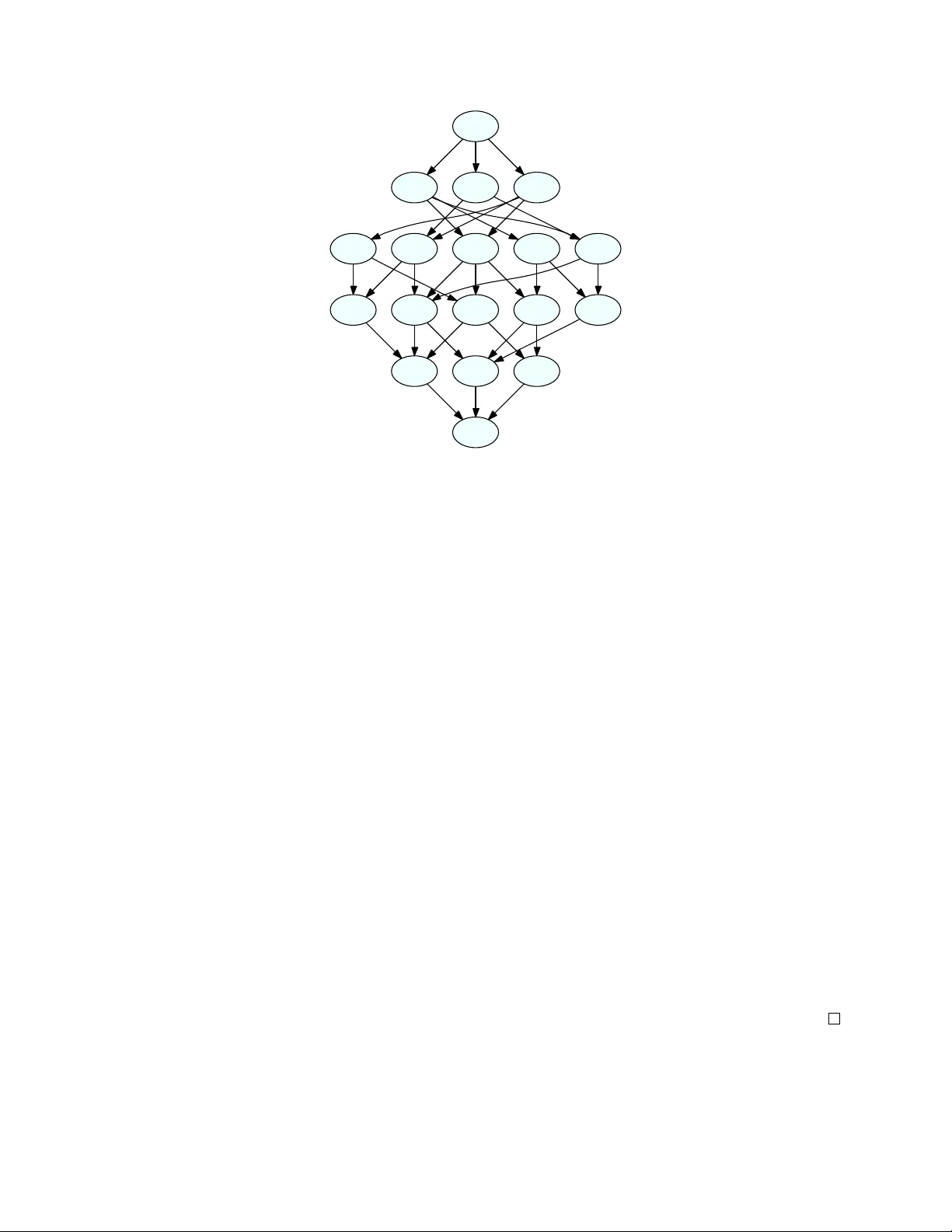
Pruning Attrib ute V alues From Data Cubes with Diamond Dicing Hazel W ebb and Owen Kaser Uni versity of Ne w Brunswick hazel.webb@unb .ca, o.kaser@computer .org Daniel Lemire Uni versit ´ e du Qu ´ ebec ` a Montr ´ eal lemire@acm.org October 28, 2018 Abstract Data stored in a data warehouse are inherently multidimensional, but most data-pruning techniques (such as iceberg and top- k queries) are unidimensional. Howe v er , analysts need to issue multidimensional queries. For example, an analyst may need to select not just the most profitable stores or—separately— the most profitable products, but simultaneous sets of stores and products fulfilling some profitability constraints. T o fill this need, we propose a new operator , the diamond dice . Because of the interaction between dimensions, the computation of diamonds is challenging. W e present the first diamond-dicing experiments on large data sets. Experiments show that we can compute diamond cubes over fact tables containing 100 million f acts in less than 35 minutes using a standard PC. terms Theory , Algorithms, Experimentation ke ywords Diamond cube, data warehouses, information retrie v al, OLAP 1 Intr oduction In signal and image processing, software subsamples data [29] for visualization, compression, or analysis purposes: commonly , images are cropped to focus the attention on a se gment. In databases, researchers ha ve proposed similar subsampling techniques [3, 14], including iceber g queries [13, 27, 33] and top-k queries [21, 22]. Formally , subsampling is the selection of a subset of the data, often with desirable properties such as representati vity , conciseness, or homogeneity . Of the subsampling techniques applicable to OLAP , only the dice operator focuses on reducing the number of attribute values without aggregation whilst retaining the original number of dimensions. Such reduced representations are sometimes of critical importance to get good online performance in Business Intelligence (BI) applications [2, 13]. Even when performance is not an issue, browsing and visu- alizing the data frequently benefit from reduced vie ws [4]. Often, business analysts are interested in distinguishing elements that are most crucial to their business, such as the k products jointly responsible for 50% of all sales, from the long tail [1]—the lesser elements. The computation of icebergs, top-k elements, or heavy-hitters has receiv ed much attention [7–9]. W e wish to generalize this type of query so that interactions between dimensions are allowed. F or example, a busi- ness analysts might want to compute a small set of stores and business hours jointly responsible for ov er 1 T able 1: Sales (in million dollars) with a 4,10 sum-diamond shaded: stores need to have sales abov e $10 mil- lion whereas product lines need sales abov e $4 million Chicago Montreal Miami Paris Berlin TV 3.4 0.9 0.1 0.9 2.0 Camcorder 0.1 1.4 3.1 2.3 2.1 Phone 0.2 8.4 2.1 4.5 0.1 Camera 0.4 2.7 6.3 4.6 3.5 Game console 3.2 0.3 0.3 2.1 1.5 D VD Player 0.2 0.5 0.5 2.2 2.3 80% of the sales. In this new setting, the head and tails of the distributions must be described using a mul- tidimensional language; computationally , the queries become significantly more difficult. Hence, analysts will often process dimensions one at a time: perhaps they would focus first on the most profitable business hours, and then aggregate sales per store, or perhaps they would find the must profitable stores and aggreg ate sales per hour . W e propose a general model, of which the unidimensional analysis is a special case, that has acceptable computational costs and a theoretical foundation. In the two-dimensional case, our proposal is a generalization of I T E R AT I V E P R U N I N G [18], a graph-trawling approach used to analyze social networks. It also generalizes iceberg queries [13, 27, 33]. T o illustrate our proposal in the BI context, consider the follo wing example. T able 1 represents the sales of different items in different locations. T ypical iceberg queries might be requests for stores having sales of at least 10 million dollars or product lines with sales of at least 4 million dollars. Howe ver , what if the analyst wants to apply both thresholds simultaneously? He might contemplate closing both some stores and some product lines. In our example, applying the constraint on stores would close Chicago, whereas applying the constraint on product lines would not terminate any product line. Ho wev er , once the shop in Chicago is closed, we see that the product line TV must be terminated which causes the closure of the Berlin store and the termination of two ne w product lines (Game console and D VD player). This multidimensional pruning query selects a subset of attribute values from each dimension that are simultaneously important. The operation is a diamond dice [32] and produces a diamond , as formally defined in Section 3. Other approaches that seek important attribute values, e.g. the Skyline operator [6, 23], Dominant Rela- tionship Analysis [20], and T op- k dominating queries [35], require dimension attribute values to be ordered, e.g. distance between a hotel and a conference venue, so that data points can be ordered. Our approach requires no such ordering. 2 Notation Notation used in this paper is tabulated belo w . 2 C a data cube σ aggregator C O U N T or S U M C dim ,j σ ( slice j of dimension dim in cube C ) | C | = P j C 1 ,j the number of allocated cells in cube C A , B cubes D i i th dimension of a data cube n i number of attribute v alues in dimension D i k number of carats k i number of carats of order 1 for D i d number of dimensions p max. number of attribute v alues per dim p i max. number of attribute v alues for D i κ ( C ) maximum carats in C C O U N T - κ ( C ) maximum carats in C , σ is C O U N T 3 Pr operties of Diamond Cubes Gi ven a database relation, a dimension D is the set of values associated with a single attribute. A cube C is the set of dimensions together with a map from some tuples in D 1 × · · · × D d to real-v alued measure v alues. W ithout losing generality , we shall assume that n 1 ≤ n 2 ≤ . . . ≤ n d , where n i is the number of distinct attribute v alues in dimension i . A slice of order δ is the set of cells we obtain when we fix a single attribute value in each of δ different dimensions. For example, a slice of order 0 is the entire cube, a slice of order 1 is the more traditional definition of a slice and so on. For a d -dimensional cube, a slice of order d is a single cell. An aggregator is a function, σ , from sets of v alues to the real numbers. Definition 1. Let σ be an aggr e gator such as S U M or C O U N T , and let k be some r eal-valued number . A cube has k carats over dimensions i 1 , . . . , i δ , if for every slice x of or der δ along dimensions i 1 , . . . , i δ , we have σ ( x ) ≥ k . W e can recov er iceberg cubes by seeking cubes having carats of order d where σ ( x ) returns the measure corresponding to cell x . The predicate σ ( x ) ≤ k could be generalized to include σ ( x ) ≥ k and other constraints. W e say that an aggregator σ is monotonically increasing if S 0 ⊂ S implies σ ( S 0 ) ≤ σ ( S ) . Similarly , σ is monotonically decreasing if S 0 ⊂ S implies σ ( S 0 ) ≥ σ ( S ) . Monotonically increasing operators include C O U N T , M A X and S U M (ov er non-negati ve measures). Monotonically decreasing operators include M I N and S U M (over non-positi ve measures). W e say a cube C 0 is r estricted fr om cube C if • they ha ve the same number of dimensions • dimension i of C 0 is a subset of dimension i of C • If in C 0 , ( v 1 , v 2 , . . . , v d ) 7→ m , then in C , ( v 1 , v 2 , . . . , v d ) 7→ m 3 Definition 2. Let A and B be two cubes with the same dimensions and measur es r estricted fr om a single cube C . Their union is denoted A ∪ B . It is the set of attributes together with their measur es, on each dimension, that appear in A , or B or both. The union of A and B is B if and only if A is contained in B : A is a subcube of B . Proposition 1. If the aggr e gator σ is monotonically incr easing, then the union of any two cubes having k carats o ver dimensions i 1 , . . . , i δ has k carats over dimensions i 1 , . . . , i δ as well. Pr oof. Any slice x of the union of A and B contains a slice x 0 from at least A or B . Since x 0 is contained in x , and σ ( x 0 ) ≥ k , we ha ve σ ( x ) ≥ k . Hence, as long as σ is monotonically increasing , there is a maximal cube having k carats ov er dimen- sions i 1 , . . . , i δ , and we call such a cube the diamond . When σ is not monotonically increasing, there may not be a unique diamond. Indeed, consider the even-numbered rows and columns of the following matrix, then consider the odd-numbered ro ws and columns. Both are maximal cubes with 2 carats (of order 1) under the S U M operator: 1 − 1 1 − 1 − 1 1 − 1 1 1 − 1 1 − 1 − 1 1 − 1 1 Because we wish diamonds to be unique, we will require σ to be The next proposition sho ws that diamonds are themselves nested. Proposition 2. The diamond having k 0 carats o ver dimensions i 1 , . . . , i δ is contained in the diamond having k carats over dimensions i 1 , . . . , i δ whenever k 0 ≥ k . Pr oof. Let A be the diamond having k carats and B be the diamond having k 0 carats. By Proposition 1, A ∪ B has at least k 0 carats, and because B is maximal, A ∪ B = B ; thus, A is contained in B . For simplicity , we only consider carats of order 1 for the rest of the paper . W e write that a cube has k 1 , k 2 , . . . , k d -carats if it has k i carats over dimension D i ; when k 1 = k 2 = . . . = k d = k we simply write that it has k carats. One consequence of Proposition 2 is that the diamonds having v arious number of carats form a lattice (see Fig. 1) under the relation “is included in. ” This lattice creates optimization opportunities: if we are gi ven the 2 , 1 -carat diamond X and the 1 , 2 -carat diamond Y , then we know that the 2 , 2 -carat diamond must lie in both X and Y . Likewise, if we hav e the 2 , 2 -carat diamond, then we know that its attribute values must be included in the diamond abov e it in the lattice (such as the 2 , 1 -carat diamond). Gi ven the size of a sum-based diamond cube (in cells), there is no upper bound on its number of carats. Ho wev er , it cannot ha ve more carats than the sum of its measures. Conv ersely , if a cube has dimension sizes n 1 , n 2 , . . . , n d and k carats, then its sum is at least k max( n 1 , n 2 , . . . , n d ) . Gi ven the dimensions of a C O U N T -based diamond cube, n 1 ≤ n 2 ≤ . . . ≤ n d − 1 ≤ n d , an upper bound for the number of carats k of a subcube is Q d − 1 i =1 n i . An upper bound on the number of carats k i for dimension 4 2,3,2 2,3,3 1,2,3 2,2,3 1,3,3 1,1,2 1,1,3 1,2,2 2,1,2 2,1,3 2,1,1 2,2,1 2,3,1 2,2,2 1,1,1 1,2,1 1,3,1 1,3,2 Figure 1: Part of the C O U N T -based diamond-cube lattice of a 2 × 2 × 2 cube i is Q d j =1 ,j 6 = i n i . An alternate (and trivial) upper bound on the number of carats in any dimension is | C | , the number of allocated cells in the cube. For sparse cubes, this bound may be more useful. Intuiti vely , a cube with many carats needs to ha ve a lar ge number of allocated cells: accordingly , the ne xt proposition provides a lo wer bound on the size of the cube given the number of carats. Proposition 3. F or d > 1 , the size S , or number of allocated cells, of a d -dimensional cube of k carats sat- isfies S ≥ k max i ∈{ 1 , 2 ,...,d } n i ≥ k d/ ( d − 1) ; mor e generally , a k 1 , k 2 , . . . , k d -carat cube has size S satisfying S ≥ max i ∈{ 1 , 2 ,...,d } k i n i ≥ ( Q i =1 ,...,d k i ) 1 / ( d − 1) . Pr oof. Pick dimension D i : the subcube has n i slices along this dimension, each with k allocated cells, proving the first item. W e hav e that k ( P i n i ) /d ≤ k max i ∈{ 1 , 2 ,...,d } n i so that the size of the subcube is at least k ( P i n i ) /d . If we prov e that P i n i ≥ dk 1 / ( d − 1) then we will hav e that k ( P i n i ) /d ≥ k d/ ( d − 1) proving the sec- ond item. This result can be shown using Lagrange multipliers. Consider the problem of minimizing P i n i gi ven the constraints Q i =1 , 2 ,...,j − 1 ,j +1 ,...,d n i ≥ k for j = 1 , 2 , . . . , d . These constraints are nec- essary since all slices must contain at least k cells. The corresponding Lagrangian is L = P i n i + P j λ j ( Q i =1 , 2 ,...,j − 1 ,j +1 ,...,d n i − k ) . By inspection, the deriv ativ es of L with respect to n 1 , n 2 , . . . , n d are zero and all constraints are satisfied when n 1 = n 2 = . . . = n d = k 1 / ( d − 1) . For these values, P i n i = dk 1 / ( d − 1) and this must be a minimum, proving the result. The more general result follo ws similarly , by proving that the minimum of P n i k i is reached when n i = ( Q i =1 ,...,d k i ) 1 / ( d − 1) /k i for all i ’ s. W e calculate the volume of a cube C as Q i = d i =1 n i and its density is the ratio of allocated cells, | C | , to the volume ( | C | / Q i = d i =1 n i ). Giv en σ , its carat-number , κ ( C ) , is the largest number of carats for which the cube has a non-empty diamond. Intuitiv ely , a small cube with many allocated cells should ha ve a large κ ( C ) . 5 One statistic of a cube C is its carat-number , κ ( C ) , which is the largest number of carats for which the cube has a non-empty diamond. Is this statistic robust? I.e., with high probability , can changing a small fraction of the data set change the statistic much? Of course, typical analyses are based on thresholds (e.g. applied to support and accuracy in rule mining), and thus small changes to the cube may not always behave as desired. Diamond dicing is no exception. For the cube C in Fig. 3 and the statistic κ ( C ) we see that diamond dicing is not robust against an adversary who can deallocate a single cell: deallocation of the second cell on the top row results means that the cube no longer contains a diamond with 2 carats. This example can be generalized. Proposition 4. F or any b , there is a cube C fr om which deallocation of any b cells r esults in a cube C 0 with κ ( C 0 ) = κ ( C ) − Ω( b ) . Pr oof. Let C be a d -dimensional cube with n i = 2 with all cells allocated. W e see that C has 2 d − 1 carats and κ ( C ) = 2 d − 1 (assume d > 1 ). Giv en b , set x = b ( d − 1) b 2 d c . Because x ≥ ( d − 1) b 2 d − 1 ≥ b 4 − 1 ∈ Ω( b ) , it suffices to show that by deallocating b cells, we can reduce the number of carats by x . By Proposition 3, we ha ve that any cube with 2 d − 1 − x carats must hav e size at least (2 d − 1 − x ) d/ ( d − 1) . When x  2 d − 1 , this size is approximately 2 d − 1 − 2 dx d − 1 , and slightly larger by the alternation of the T aylor expansion. Hence, if we deallocate at least 2 dx d − 1 cells, the number of carats must go down by at least x . But x = b ( d − 1) b 2 d c ⇒ x ≤ ( d − 1) b 2 d ⇒ b ≥ 2 dx d − 1 which shows the result. It is always possible to choose d large enough so that x  2 d − 1 irrespecti ve of the v alue b . Con versely , in Fig. 3 we might allocate the cell above the bottom-right corner , thereby obtaining a 2-carat diamond with all 2 n + 1 cells. Compared to the original case with a 4-cell 2-carat diamond, we see that a small change effects a v ery dif ferent result. Diamond dicing is not, in general, rob ust. Ho wev er , it is perhaps more reasonable to follow Pensa and Boulicaut [28] and ask whether κ appears, e xperimentally , to be robust against random noise on realistic data sets. W e return to this in Subsection 6.5. Many OLAP aggregators are distributi ve, algebraic and linear . An aggregator σ is distributive [16] if there is a function F such that for all 0 ≤ k < n − 1 , σ ( a 0 , . . . , a k , a k +1 , . . . , a n − 1 ) = F ( σ ( a 0 , . . . , a k ) , σ ( a k +1 , . . . , a n − 1 )) . An aggregator σ is algebraic if there is an intermediate tuple-v alued distributi ve range-query function G from which σ can be computed. An algebraic example is A V E R AG E : giv en the tuple ( C O U N T , S U M ) , one can compute A V E R AG E by a ratio. In other words, if σ is an algebraic function then there must exist G and F such that G ( a 0 , . . . , a k , a k +1 , . . . , a n − 1 ) = F ( G ( a 0 , . . . , a k ) , G ( a k +1 , . . . , a n − 1 )) . An algebraic aggregator σ is linear [19] if the corresponding intermediate query G satisfies G ( a 0 + αd 0 , . . . , a n − 1 + αd n − 1 ) = G ( a 0 , . . . , a n − 1 ) + αG ( d 0 , . . . , d n − 1 ) for all arrays a, d , and constants α . S U M and C O U N T are linear functions; M A X is not linear . 6 4 Related Pr oblems In this section, we discuss four problems, three of which are NP-hard, and show that the diamond—while perhaps not pro viding an e xact solution—is a good starting point. The first two problems, T rawling the W eb for Cyber-communities and Largest Perfect Subcube, assume use of the aggregator C O U N T whilst for the remaining problems we assume S U M . 4.1 T rawling the W eb f or Cyber -communities In 1999, Kumar et al. [18] introduced the I T E R A T I V E P R U N I N G algorithm for discovering emerging com- munities on the W eb . They model the W eb as a directed graph and seek large dense bipartite subgraphs or cores, and therefore their problem is a 2-D version of our problem. Although their paper has been widely cited [30, 34], to our knowledge, we are the first to propose a multidimensional extension to their problem suitable for use in more than two dimensions and to pro vide a formal analysis. 4.2 Largest P erfect Cube A perfect cube contains no empty cells, and thus it is a diamond. Finding the largest perfect diamond is NP-hard. A motiv ation for this problem is found in Formal Concept Analysis [15], for example. Proposition 5. F inding a perfect subcube with lar gest volume is NP-har d, even in 2-D. Pr oof. A 2-D cube is essentially an unweighted bipartite graph. Thus, a perfect subcube corresponds directly to a biclique —a clique in a bipartite graph. Finding a biclique with the largest number of edges has been sho wn NP-hard by Peeters [26], and this problem is equi valent to finding a perfect subcube of maximum volume. Finding a diamond might be part of a sensible heuristic to solv e this problem, as the ne xt lemma suggests. Lemma 1. F or C O U N T -based carats, a perfect subcube of size n 1 × n 2 × . . . × n d is contained in the Q d i =1 n i / max i n i -carat diamond and in the k 1 , k 2 , . . . , k d -carat diamond wher e k i = Q d j =1 n j /n i . This helps in two ways: if there is a nontrivial diamond of the specified size, we can search for the perfect subcube within it; howe ver , if there is only an empty diamond of the specified size, there is no perfect subcube. 4.3 Densest Cube with Limited Dimensions In the OLAP context, giv en a cube, a user may ask to “find the subcube with at most 100 attribute values per dimension. ” Meanwhile, he may want to keep as much of the cube as possible. W e call this problem D E N S E S T C U B E W I T H L I M I T E D D I M E N S I O N S (DCLD), which we formalize as: pick min( n i , p ) attribute v alues for dimension D i , for all i ’ s, so that the resulting subcube is maximally dense. Intuiti vely , a densest cube should at least contain a diamond. W e proceed to show that a sufficiently dense cube always contains a diamond with a lar ge number of carats. 7 Proposition 6. If a cube does not contain a k -car at subcube, then it has at most 1 + ( k − 1) P d i =1 ( n i − 1) allocated cells. Hence, it has density at most (1 + ( k − 1) P d i =1 ( n i − 1)) / Q d i =1 n i . Mor e gener ally , a cube that does not contain a k 1 , k 2 , . . . , k d -carat subcube has size at most 1 + P d i =1 ( k i − 1)( n i − 1) and density at most (1 + P d i =1 ( k i − 1)( n i − 1)) / Q d i =1 n i . Pr oof. Suppose that a cube of dimension at most n 1 × n 2 × . . . × n d contains no k -carat diamond. Then one slice must contain at most k − 1 allocated cells. Remove this slice. The amputated cube must not contain a k -carat diamond. Hence, it has one slice containing at most k − 1 allocated cells. Remove it. This iterativ e process can continue at most P i ( n i − 1) times before there is at most one allocated cell left: hence, there are at most ( k − 1) P i ( n i − 1) + 1 allocated cells in total. The more general result follows similarly . The follo wing corollary follows tri vially from Proposition 6: Corollary 1. A cube of size gr eater than 1 + ( k − 1) P d i =1 ( n i − 1) allocated cells, that is, having density gr eater than 1 + ( k − 1) P d i =1 ( n i − 1) Q d i =1 n i , must contain a k -carat subcube. If a cube contains mor e than 1 + P d i =1 ( k i − 1)( n i − 1) allocated cells, it must contain a k 1 , k 2 , . . . , k d -carat subcube . Solving for k , we ha ve a lo wer bound on the maximal number of carats: κ ( C ) ≥ | C | / P i ( n i − 1) − 3 . W e also hav e the following corollary to Proposition 6: Corollary 2. Any solution of the DCLD pr oblem having density above 1 + ( k − 1) P d i =1 (min( n i , p ) − 1) Q d i =1 min( n i , p ) ≤ 1 + ( k − 1) d ( p − 1) Q d i =1 n i must intersect with the k -carat diamond. When n i ≥ p for all i , then the density threshold of the previous corollary is (1 + ( k − 1) d ( p − 1)) /p d : this v alue goes to zero exponentially as the number of dimensions increases. W e might hope that when the dimensions of the diamond coincide with the required dimensions of the densest cube, we would hav e a solution to the DCLD problem. Alas, this is not true. Consider the 2-D cube in Fig. 2. The bottom-right quadrant forms the largest 3-carat subcube. In the bottom-right quadrant, there are 15 allocated cells whereas in the upper-left quadrant there are 16 allocated cells. This prov es the next result. Lemma 2. Even if a diamond has exactly min( n i , p i ) attribute values for dimension D i , for all i ’ s, it may still not be a solution to the DCLD pr oblem. W e are interested in large data sets; the ne xt theorem shows that solving DCLD and HCLD is dif ficult. Theorem 1. The DCLD and HCLD pr oblems ar e NP-har d. 8 1 1 1 1 1 1 1 1 1 1 1 1 1 1 1 1 1 1 1 1 1 1 1 1 1 1 1 1 1 1 1 Figure 2: Example showing that a diamond (bottom-right quadrant) may not ha ve optimal density . Pr oof. The E X AC T B A L A N C E D P R I M E N O D E C A R D I N A L I T Y D E C I S I O N P R O B L E M (EBPNCD) is NP-complete [10]— for a gi ven bipartite graph G = ( V 1 , V 2 , E ) and a number p , does there e xist a biclique U 1 and U 2 in G such that | U 1 | = p and | U 2 | = p ? Gi ven an EBPNCD instance, construct a 2-D cube where each value of the first dimension corresponds to a v ertex of V 1 , and each v alue of the second dimension corresponds to a verte x of V 2 . Fill cell corresponding to v 1 , v 2 ∈ V 1 × V 2 with a measure v alue if and only if v 1 is connected to v 2 . The solution of the DCLD problem applied to this cube with a limit of p will be a biclique if such a biclique exists. It follo ws that HCLD is also NP-hard by reduction of DCLD. 4.4 Hea viest Cube with Limited Dimensions In the OLAP conte xt, gi ven a cube, a user may ask to “find a subcube with 10 attrib ute v alues per dimension. ” Meanwhile, he may want the resulting subcube to hav e maximal av erage—he is, perhaps, looking for the 10 attributes from each dimension that, in combination, give the greatest profit. Note that this problem does not restrict the number of attribute v alues ( p ) to be the same for each dimension. W e call this problem the H E A V I E S T C U B E W I T H L I M I T E D D I M E N S I O N S (HCLD), which we formalize as: pick min( n i , p i ) attrib ute v alues for dimension D i , for all i ’ s, so that the resulting subcube has maximal av erage. W e have that the HCLD must intersect with diamonds. Theorem 2. Using the S U M operator , a cube without any k 1 , k 2 , . . . , k d -carat subcube has sum less than P d i =1 ( n i + 1) k i + max( k 1 , k 2 , . . . , k d ) wher e the cube has size n 1 × n 2 × . . . × n d . Pr oof. Suppose that a cube of dimension n 1 × n 2 × . . . × n d contains no k 1 , k 2 , . . . , k d -sum-carat cube. Such a cube must contain at least one slice with sum less than k , remove it. The remainder must also not contain a k -sum-carat cube, remove another slice and so on. This process may go on at most P d i =1 ( n i + 1) times before there is only one cell left. Hence, the sum of the cube is less than P d i =1 ( n i + 1)( k i ) + max( k 1 , k 2 , . . . , k d ) . Corollary 3. Any solution to the HCLD pr oblem having averag e gr eater than P d i =1 ( n i + 1) k i + max( k 1 , k 2 , . . . , k d ) Q d i =1 n i 9 must intersect with the k 1 , k 2 , . . . , k d -sum-carat diamond. 5 Algorithm W e hav e developed and implemented an algorithm for computing diamonds. Its overall approach is illus- trated by Example 1. That approach is to repeatedly identify an attribute value that cannot be in the diamond, and then (possibly not immediately) remove the attribute v alue and its slice. The identification of “bad” attribute values is done conservati vely , in that they are known already to hav e a sum less than required ( σ is sum), or insufficient allocated cells ( σ is count). When the algorithm terminates, we are left with only attribute v alues that meet the condition in ev ery slice: a diamond. Example 1. Suppose we seek a 4,10-carat diamond in T able 1 using Algorithm 1. On a first pass, we can delete the attribute values “Chicago” and “TV” because their r espective slices have sums below 10 and 4. On a second pass, value “Berlin, ” “Game console” and “D VD” can be remo ved because the sums of their slices wer e reduced by the r emoval of the values “Chicago” and “TV . ” The algorithm then terminates. Algorithms based on this approach will always terminate, though the y might sometimes return an empty cube. The correctness of our algorithm is guaranteed by the following result. Theorem 3. Algorithm 1 is correct, that is, it always r eturns the k 1 , k 2 , . . . , k d -carat diamond. Pr oof. Because the diamond is unique, we need only show that the result of the algorithm, the cube A , is a diamond. If the result is not the empty cube, then dimension D i has at least value k i per slice, and hence it has k i carats. W e only need to show that the result of Algorithm 1 is maximal: there does not exist a larger k 1 , k 2 , . . . , k d -carat cube. Suppose A 0 is such a larger k 1 , k 2 , . . . , k d -carat cube. Because Algorithm 1 begins with the whole cube C , there must be a time when, for the first time, one of the attribute values of C belonging to A 0 but not A is deleted. This attribute is not written to the output file because its corresponding slice of dimension dim had v alue less than k dim . At the time of deletion, this attribute’ s slice cannot hav e obtained more cells after it had been deleted, so it still has value less than k dim . Let C 0 be the cube at the instant before the attribute is deleted, with all attribute values deleted so far . W e see that C 0 is larger than or equal to A 0 and therefore, slices in C 0 corresponding to attribute values of A 0 along dimension dim must have more than k dim carats. Therefore, we hav e a contradiction and must conclude that A 0 does not exist and that A is maximal. F or simplicity of exposition, in the rest of the paper , we assume that the number of carats is the same f or all dimensions. Our algorithm employs a preprocessing step that iterates over the input file creating d hash tables that map attributes to their σ -values. When σ = C O U N T , the σ -values for each dimension form a histogram, which might be precomputed in a DBMS. These values can be updated quickly as long as σ is linear: aggregators like S U M and C O U N T are good candidates. If the cardinality of any of the dimensions is such that hash tables cannot be stored in main memory , then a file-based set of hash tables could be constructed. Howe ver , given a d -dimensional cube, 10 input : file inFile containing d − dimensional cube C , integer k > 0 output : the diamond data cube // preprocessing scan computes σ values for each slice f oreach dimension i do Create hash table ht i f oreach attribute value v in dimension i do if σ ( slice for value v of dimension i in C ) ≥ k then ht i ( v ) = σ ( slice for v alue v of dimension i in C ) end end end stable ← false while ¬ stable do Create ne w output file outFile // iterate main loop stable ← true f oreach r ow r of inFile do ( v 1 , v 2 , . . . , v d ) ← r if v i ∈ dom ht i , for all 1 ≤ i ≤ d then write r to outFile else f or j ∈ { 1 , . . . , i − 1 , i + 1 , . . . , d } do if v j ∈ dom ht j then ht j ( v j ) = ht j ( v j ) − σ ( { r } ) if ht j ( v j ) < k then remov e v j from dom ht j end end end stable ← false end end if ¬ stable then inFile ← outFile // prepare for another iteration end end retur n outFile Algorithm 1 : Diamond dicing for relationally stored cubes. Each iteration, less data is processed. 11 1 1 1 1 1 1 1 1 . . . . . . 1 1 1 1 Figure 3: An n × n cube with 2 n allocated cells (each indicated by a 1) and a 2-carat diamond in the upper left: it is a difficult case for an iterati ve algorithm. there are only P d i =1 n i slices and so the memory usage is O ( P d i =1 n i ) : for our tests, main memory hash tables suf fice. Algorithm 1 reads and writes the files sequentially from and to disk and does not require potentially expensi ve random access, making it a candidate for a data parallel implementation in the future. Let I be the number of iterations through the input file till conv ergence; ie no more deletions are done. V alue I is data dependent and (by Fig. 3) is Θ( P i n i ) in the worst case. In practice, we do not expect I to be nearly so large, and w orking with our largest “real w orld” data sets we nev er found I to exceed 100. Algorithm 1 runs in time O( I d | C | ); each attrib ute v alue is deleted at most once. In many cases, the input file decreases substantially in the first fe w iterations and those cubes will be processed f aster than this bound suggests. The more carats we seek, the faster the file will decrease initially . The speed of con ver gence of Algorithm 1 and indeed the size of an ev entual diamond may depend on the data-distribution ske w . Cell allocation in data cubes is very ske wed and frequently follows Zipfian/- Pareto/zeta distributions [24]. Suppose the number of allocated cells C dim ,i in a giv en slice i follows a zeta distribution: P ( C dim ,i = j ) ∝ j − s for s > 1 . The parameter s is indicativ e of the skew . W e then hav e that P ( C dim ,i < k i ) = P k i − 1 j =1 j − s / P ∞ j =1 j − s = P k i ,s . The expected number of slices marked for deletion after one pass of over all dimensions using σ = C O U N T , prior to any slice deletion, is thus P d i =1 n i P k i ,s . This quantity grows fast to P d i =1 n i (all slices marked for deletion) as s grows (see Fig. 4). For S U M -based diamonds, we not only have the skew of the cell allocation, but also the skew of the measures to accelerate con vergence. In other words, we expect Algorithm 1 to con verge quickly over real data sets, b ut more slo wly ov er synthetic cubes generated using uniform distributions. 5.1 Finding the Largest Number of Carats The determination of κ ( C ) , the lar gest v alue of k for which C has a non-tri vial diamond, is a special case of the computation of the diamond-cube lattice (see Proposition 2). Identifying κ ( C ) may help guide analysis. T wo approaches hav e been identified: 1. Assume σ = C O U N T . Set the parameter k to 1 + the lower bound (provided by Proposition 6 or Theorem 2) and check whether there is a diamond with k carats. Repeat, incrementing k , until an empty cube results. At each step, Proposition 2 says we can start from the cube from the previous iteration, rather than from C . When σ is S U M , there are two additional complications. First, the v alue 12 0.1 0.2 0.3 0.4 0.5 0.6 0.7 0.8 0.9 1 1 2 3 4 5 6 7 8 9 10 expected fraction of the slices deleted s k=2 k=5 k=10 Figure 4: Expected fraction of slices marked for deletion after one pass under a zeta distribution for v arious v alues of the ske w parameter s . of k can grow large if measure v alues are large. Furthermore, if some measures are not integers, the result need not be an integer (hence we would compute b κ ( C ) c by applying this method, and not κ ( C ) ). 2. Assume σ = C O U N T . Observe that κ ( C ) is in a finite interval. W e have a lo wer bound from Proposi- tion 6 or Theorem 2 and an upper bound Q d − 1 i =1 n i or | C | . (If this upper bound is unreasonably large, we can either use the number of cells in our current cube, or we could start with the lower bound and repeatedly double it.) Execute the diamond-dicing algorithm and set k to a value determined by a binary search over its valid range. Every time the lower bound changes, we can make a copy of the resulting diamond. Thus, each time we test a new midpoint k , we can begin the computation from the copy (by Proposition 2). If σ is S U M and measures are not inte ger values, it might be dif ficult to kno w when the binary search has con verged e xactly . W e believe the second approach is better . Let us compare one iteration of the first approach (which begins with a k -carat diamond and seeks a k + 1 -carat diamond) and a comparable iteration of the second approach (which begins with a k -carat diamond and seeks a ( k + k upper ) / 2 -carat diamond). Both will end up making at least one scan, and probably se veral more, through the k -carat diamond. Now , we experimentally observe that k values that slightly exceed κ ( C ) tend to lead to se veral times more scans through the cube than with other v alues of k . Our first approach will mak e only one such unsuccessful attempt, whereas the binary search would typically make sev eral unsuccessful attempts while narrowing in on κ ( C ) . Nev ertheless, we belie ve the fe wer attempts will far outweigh this ef fect. W e recommend binary search, giv en that it will find κ ( C ) in O( log κ ( C ) ) iterations. If one is willing to accept an approximate answer for κ ( C ) when aggregating with S U M , a similar ap- proach can be used. 5.2 Diamond-Based Heuristic f or DCLD In Section 4.4, we noted that a diamond with the appropriate shape will not necessarily solve the DCLD problem. Nevertheless, when we examined many small random cubes, the solutions typically coincided. Therefore, we suggest diamond dicing as a heuristic for DCLD. 13 A heuristic for DCLD can start with a diamond and then refine its shape. Our heuristic first finds a diamond that is only somewhat too lar ge, then removes slices until the desired shape is obtained. See Algorithm 2. input : d -dimensional cube C , integers p 1 , p 2 , . . . p d output : Cube with size p 1 × p 2 × . . . × p d // Use binary search to find k Find max k where the k -carat diamond ∆ has shape p 0 1 × p 0 2 × . . . × p 0 d , where ∀ i.p 0 i ≥ p i f or i ← 1 to d do Sort slices of dimension i of ∆ by their σ values Retain only the top p i slices and discard the remainder from ∆ end retur n ∆ Algorithm 2 : DCLD heuristic that starts from a diamond. 6 Experiments W e wish to show that diamonds can be computed ef ficiently . W e also want to re view experimentally some of the properties of diamonds including their density (count-based diamonds) and the range of v alues the carats may take in practice. Finally , we want to provide some evidence that diamond dicing can serve as the basis for a DCLD heuristic. 6.1 Data Sets W e experimented with diamond dicing on several different data sets, some of whose properties are laid out in T ables 2 and 5. Cubes TW1 , TW2 and TW3 were extracted from TWEED [12], which contains over 11,000 records of e vents related to internal terrorism in 18 countries in W estern Europe between 1950 and 2004. Of the 52 di- mensions in the TWEED data, 37 were measures since they decomposed the number of people killed/injured into all the affected groups. Cardinalities of the dimensions ranged from 3 to 284. Cube TW1 retained dimensions Country , Y ear , Action and T arget with cardinalities of 16 × 53 × 11 × 11. For cubes TW2 and TW3 all dimensions not deemed measures were retained. Cubes TW2 and TW3 were rolled-up and stored T able 2: Real data sets used in experiments TWEED Netflix Census income cube TW1 TW2 TW3 NF1 NF2 C1 C2 dimensions 4 15 15 3 3 28 28 | C | 1957 4963 4963 100,478,158 100,478,158 196054 196054 P d i =1 n i 88 674 674 500,137 500,137 533 533 measure count count killed count rating stocks wage iters to con verge 6 10 3 19 40 6 4 κ 38 37 85 1,004 3,483 99,999 9,999 14 in a MySQL database using the following query and the resulting tables were exported to comma separated files. A similar process was follo wed for TW1 . T able 3 lists the details of the TWEED data. INSERT INTO t w e e d 1 5 ( d 1 , d 2 , d 3 , d 4 , d 5 , d 6 , d 7 , d 8 , d 3 1 , d 3 2 , d 3 3 , d 3 4 , d 5 0 , d 5 1 , d 5 2 , d 4 9 ) S EL EC T d 1 , d 2 , d 3 , d 4 , d 5 , d 6 , d 7 , d 8 , d 3 1 , d 3 2 , d 3 3 , d 3 4 , d 5 0 , d 5 1 , d 5 2 , sum ( d 9 ) F R O M ‘ t w e e d ‘ G R O U P B Y ( d 1 , d 2 , d 3 , d 4 , d 5 , d 6 , d 7 , d 8 , d 3 1 , d 3 2 , d 3 3 , d 3 4 , d 5 0 , d 5 1 , d 5 2 ) W e also processed the Netflix data set [25], which has dimensions: MovieID × UserID × Date × Rating ( 17766 × 480189 × 2182 × 5 ). Each ro w in the fact table has a distinct pair of values (MovieID, UserID). W e extracted two 3-D cubes NF1 and NF2 both with about 10 8 allocated cells using dimensions MovieID, UserID and Date. For NF2 we use Rating as the measure and the S U M aggregator , whereas NF1 uses the C O U N T aggregator . The Netflix data set is the largest openly a vailable mo vie-rating database ( ≈ 2 GiB). Our third real data set, Census-Income, comes from the UCI KDD Archiv e [17]. The cardinalities of the dimensions ranged from 2 to 91 and there were 199,523 records. W e rolled-up the original 41 dimensions to 27 and used two measures, income from stocks( C1 ) and hourly wage( C2 ). The MySQL query used to generate cube C1 follows. Note that the dimension numbers map to those gi ven in the census-income.names file [17]. Details are provided in table 4 INSERT INTO c e n s u s i n c o m e s t o c k s ( ‘ d 0 ‘ , ‘ d 1 ‘ , ‘ d 2 ‘ , ‘ d 3 ‘ , ‘ d 4 ‘ , ‘ d 6 ‘ , ‘ d 7 ‘ , ‘ d 8 ‘ , ‘ d 9 ‘ , ‘ d 1 0 ‘ , ‘ d 1 2 ‘ , ‘ d 1 3 ‘ , ‘ d 1 5 ‘ , ‘ d 2 1 ‘ , ‘ d 2 3 ‘ , ‘ d 2 4 ‘ , ‘ d 2 5 ‘ , ‘ d 2 6 ‘ , ‘ d 2 7 ‘ , ‘ d 2 8 ‘ , ‘ d 2 9 ‘ , ‘ d 3 1 ‘ , ‘ d 3 2 ‘ , ‘ d 3 3 ‘ , ‘ d 3 4 ‘ , ‘ d 3 5 ‘ , ‘ d 3 8 ‘ , ‘ d 1 8 ‘ ) S EL EC T ‘ d 0 ‘ , ‘ d 1 ‘ , ‘ d 2 ‘ , ‘ d 3 ‘ , ‘ d 4 ‘ , ‘ d 6 ‘ , ‘ d 7 ‘ , ‘ d 8 ‘ , ‘ d 9 ‘ , ‘ d 1 0 ‘ , ‘ d 1 2 ‘ , ‘ d 1 3 ‘ , ‘ d 1 5 ‘ , ‘ d 2 1 ‘ ‘ d 2 3 ‘ , ‘ d 2 4 ‘ , ‘ d 2 5 ‘ , ‘ d 2 6 ‘ , ‘ d 2 7 ‘ , ‘ d 2 8 ‘ , ‘ d 2 9 ‘ , ‘ d 3 1 ‘ , ‘ d 3 2 ‘ , ‘ d 3 3 ‘ , ‘ d 3 4 ‘ , ‘ d 3 5 ‘ , ‘ d 3 8 ‘ , s um ( ‘ d 1 8 ‘ ) F R O M c e n s u s i n c o m e G R O U P B Y ‘ d 0 ‘ , ‘ d 1 ‘ , ‘ d 2 ‘ , ‘ d 3 ‘ , ‘ d 4 ‘ , ‘ d 6 ‘ , ‘ d 7 ‘ , ‘ d 8 ‘ , ‘ d 9 ‘ , ‘ d 1 0 ‘ , ‘ d 1 2 ‘ , ‘ d 1 3 ‘ , ‘ d 1 5 ‘ , ‘ d 2 1 ‘ , ‘ d 2 3 ‘ , ‘ d 2 4 ‘ , ‘ d 2 5 ‘ , ‘ d 2 6 ‘ , ‘ d 2 7 ‘ , ‘ d 2 8 ‘ , ‘ d 2 9 ‘ , ‘ d 3 1 ‘ , ‘ d 3 2 ‘ , ‘ d 3 3 ‘ , ‘ d 3 4 ‘ , ‘ d 3 5 ‘ , ‘ d 3 8 ‘ ; W e also generated synthetic data. As has already been stated, cell allocation in data cubes is skewed. W e modelled this by generating values in each dimension that follo wed a po wer distribution. The values in dimension i were generated as b n i u 1 /a c where u ∈ [0 , 1] is a uniform distribution. For a = 1 , this function generates uniformly distributed v alues. The dimensions are statistically independent. W e picked the first 250,000 distinct facts. Since cubes S2A and S3A were generated with close to 250,000 distinct facts we decided to keep them all. The cardinalities for all synthetic cubes are laid out in T able 6. All experiments on our synthetic data were done using the measure C O U N T . 15 T able 3: Measures and dimensions of TWEED data. Shaded dimensions are those retained for TW1 . All dimensions were retained for cubes TW2 and TW3 (with total people killed as its measure) Dimension Dimension cardinality d1 Day 32 d2 Month 13 d3 Y ear 53 d4 Country 16 d5 T ype of agent 3 d6 Acting group 287 d7 Regional conte xt of the agent 34 d8 T ype of action 11 d31 State institution 6 d32 Kind of action 4 d33 T ype of action by state 7 d34 Group against which the state action is directed 182 d50 Group’ s attitude tow ards state 6 d51 Group’ s ideological character 9 d52 T arget of action 11 Measure d49 total people killed people from the acting group military police ci vil servants politicians business e xecuti ves trade union leaders clergy other militants ci vilians total people injured acting group military police ci vil servants politicians business trade union leaders clergy other militants ci vilians total people killed by state institution group members other people total people injured by state institution group members other people arrests con victions ex ecutions total killed by non-state group at which the state directed an action people from state institution others total injured by non-state group people from state institution others 16 T able 4: Census Income data: dimensions and cardinality of dimensions. Shaded dimensions and mea- sures retained for cubes C1 and C2 . Dimension numbering maps to those described in the file census- income.names [17] Dimension Dimension cardinality d0 age 91 d1 class of w orker 9 d2 industry code 52 d3 occupation code 47 d4 education 17 d6 enrolled in education last week 3 d7 marital status 7 d8 major industry code 24 d9 major occupation code 15 d10 race 5 d12 sex 2 d13 member of a labour union 3 d15 full or part time employment status 8 d21 state of pre vious residence 51 d23 detailed household summary in household 8 d24 migration code - change in msa 10 d25 migration code - change in region 9 d26 migration code - mov ed within region 10 d27 li ve in this house 1 year ago 3 d28 migration pre vious residence in sunbelt 4 d29 number of persons worked for emplo yer 7 d31 country of birth father 43 d32 country of birth mother 43 d33 country of birth self 43 d34 citizenship 5 d35 o wn business or self emplo yed 3 d38 weeks worked in year 53 d11 hispanic origin 10 d14 reason for unemployment 6 d19 tax filer status 6 d20 region of pre vious residence 6 d22 detailed household and family status 38 ignored instance weight d30 family members under 18 5 d36 fill inc questionnaire for veteran’ s admin 3 d37 veteran’ s benefits 3 d39 year 2 ignored classification bin Measure Cube d18 di vidends from stocks C1 d5 w age per hour C2 d16 capital gains d17 capital losses 17 T able 5: Synthetic data sets used in experiments cube S1A S1B S1C S2A S2B S2C S3A S3B S3C dimensions 4 4 4 8 8 8 16 16 16 ske w factor 0.02 0.2 1.0 0.02 0.2 1.0 0.02 0.2 1.0 | C | 250k 250k 250k 251k 250k 250k 262k 250k 250k P d i =1 n i 11,106 11,098 11,110 22,003 22,195 22,220 38,354 44,379 44,440 iters to con verge 12 9 2 6 12 12 8 21 6 κ 135 121 30 133 32 18 119 8 15 T able 6: Dimensional cardinalities for our synthetic data cubes Cube Dimensional cardinalities S1A 6 × 100 × 1000 × 10000 S1B 2 × 100 × 1000 × 9996 S1C 10 × 100 × 1000 × 10000 S2A 10 × 100 × 1000 × 9881 × 10 × 100 × 1000 × 9902 S2B 10 × 100 × 1000 × 9987 × 10 × 100 × 1000 × 9988 S2C 10 × 100 × 1000 × 10000 × 10 × 100 × 1000 × 10000 S3A 10 × 100 × 1000 × 8465 × 10 × 100 × 1000 × 8480 × 10 × 100 × 1000 × 8502 × 10 × 100 × 1000 × 8467 S3B 10 × 100 × 1000 × 9982 × 10 × 100 × 1000 × 9987 × 10 × 100 × 1000 × 9988 × 10 × 100 × 1000 × 9982 S3C 10 × 100 × 1000 × 10000 × 10 × 100 × 1000 × 10000 × 10 × 100 × 1000 × 10000 × 10 × 100 × 1000 × 10000 All experiments were carried out on a Linux-based (Ubuntu 7.04) dual-processor machine with Intel Xeon (single core) 2.8 GHz processors with 2 GiB RAM. It had one disk, a Seagate Cheetah ST373453LC (SCSI 320, 15 kRPM, 68 GiB), formatted to the ext3 filesystem. Our implementation was done with Sun’ s SDK 1.6.0 and to handle the large hash tables generated when processing Netflix, we set the maximum heap size for the JVM to 2 GiB. 6.2 Iterations to Con vergence Algorithm 1 required 19 iterations and an av erage of 35 minutes to compute the 1004-carat κ -diamond for NF1 . Ho we ver it took 50 iterations and an a verage of 60 minutes to determine that there was no 1005-carat diamond. The preprocessing time for NF1 was 22 minutes. For a comparison, sorting the Netflix comma- separated data file took 29 minutes. T imes were averaged over 10 runs. Fig. 5 shows the number of cells present in the diamond after each iteration for 1004–1006 carats. The curve for 1006 reaches zero first, follo wed by that for 1005. Since κ ( NF1 ) = 1004 , that curve stabilizes at a nonzero value. W e see a similar result for TW2 in Fig. 6 where κ is 37. It takes longer to reach a critical point when k only slightly exceeds κ . As stated in Section 5, the number of iterations required until conv ergence for all our real and synthetic 18 0 5e+006 1e+007 1.5e+007 2e+007 0 10 20 30 40 50 cells left iteration 1004 carats 1005 carats 1006 carats Figure 5: Cells remaining after each iteration of Algorithm 1 on NF1 , computing a 1004-, 1005- and 1006- carat diamonds. 0 500 1000 1500 2000 2500 3000 1 2 3 4 5 6 7 8 9 10 11 cells left iteration 35 carats 36 carats 37 carats 38 carats 39 carats 40 carats Figure 6: Cells remaining after each iteration, TW2 cubes was far fewer than the upper bound, e.g. cube S2B : 2,195 (upper bound) and 12 (actual). W e had expected to see the uniformly distributed data taking longer to con verge than the skewed data. This was not the case. It may be that a clearer difference would be apparent on larger synthetic data sets. This will be in vestigated in future experiments. 6.3 Largest Carats According to Proposition 6, C O U N T - κ ( NF1 ) ≥ 197 . Experimentally , we determined that it was 1004. By the definition of the carat, it means we can extract a subset of the Netflix data set where each user entered at least 1004 ratings on movies rated at least 1004 times by these same users during days where there were at least 1004 ratings by these same users on these same movies. The 1004-carat diamond had dimensions 3082 × 6833 × 1351 and 8,654,370 cells, for a density of about 3 × 10 − 4 or two orders of magnitude denser than the original cube. The presence of such a large diamond was surprising to us. W e belie ve nothing similar has been observed about the Netflix data set before [5]. Comparing the two methods in Section 5.1, we see that sequential search would try 809 values of k before identifying κ . Howe ver , binary search would try 14 values of k (although 3 are between 1005 and 1010, where perhaps double or triple the normal number of iterations are required). T o test the time difference for the tw o methods, we used cube TW1 . W e executed a binary search, repeatedly doubling our lo wer bound to obtain the upper limit, and thus until we established the range where κ must e xist. Whenev er we e xceeded 19 0 20 40 60 80 100 120 140 160 S1A S1B S1C S2A S2B S2C S3A S3B S3C TW1 TW2 carats cube Lower bounds Actual value Figure 7: Comparison between estimated κ , based on the lower bounds from Proposition 6, and number of ( C O U N T -based) carats found. κ , a copy of the original data was used for the next step. Ev en with this copying step and the unnecessary recomputation from the original data, the time for binary search av eraged only 2.75 seconds. Whereas a sequential search, that started with the lo wer bound and increased k by one, av eraged 9.854 seconds over ten runs. Fig. 7 shows our lower bounds on κ , given the dimensions and numbers of allocated cells in each cube, compared with their actual κ values. The plot indicates that our lower bounds are further away from actual v alues as the ske w of the cube increases for the synthetic cubes. Also, we are further a way from κ for TW2 , a cube with 15 dimensions, than for TW1 . F or uniformly-distributed cubes S1C , S2C and S3C there was no real difference in density between the cube and its diamond. Howe ver , all other diamonds experienced an increase of between 5 and 9 orders of magnitude. Diamonds found in C1 , C2 , NF2 and TW3 captured 0.35%, 0.09%, 66.8% and 0.6% of the o verall sum for each cube respectiv ely . The very small fraction captured by the diamond for TW3 can be explained by the fact that κ ( TW3 ) is based on a diamond that has only one cell, a bombing in Bologna in 1980 that killed 85 people. Similarly , the diamond for C2 also comprised a single cell. 6.4 Effectiveness of DCLD Heuristic T o test the effecti veness of our diamond-based DCLD heuristic (Subsection 5.2), we used cube TW1 and set the parameter p to 5. W e were able to establish quickly that the 38-carat diamond was the closest to satisfying this constraint. It had density of 0.169 and cardinalities of 15 × 7 × 5 × 8 for the attrib ute values; year , country , action and target. The solution we generated to this DCLD ( p = 5 ) problem had exactly 5 attribute v alues per dimension and density of 0.286. Since the DCLD problem is NP-complete, determining the quality of the heuristic poses difficulties. W e are not aware of any known approximation algorithms and it seems dif ficult to formulate a suitably fast ex- act solution by , for instance, branch and bound. Therefore, we also implemented a second computationally expensi ve heuristic, in hope of finding a high-quality solution with which to compare our diamond-based heuristic. This heuristic is based on local search from an intuitiv ely reasonable starting state. (A greedy steepest-descent approach is used; states are ( h A 1 , A 2 , . . . , A d i , where | A i | = p i , and the local neighbour- hood of such a state is h A 0 1 , A 0 2 , . . . , A 0 d i , where A i = A 0 i except for one v alue of i , where | A i ∩ A 0 i | = p i − 1 . 20 The starting state consists of the most frequent p i v alues from each dimension i . Our implemention actually requires the i t h local move be chosen along dimension i mo d d , although if no such mov e brings improve- ment, no mov e is made.) input : d -dimensional cube C , integers p 1 , p 2 , . . . p d output : Cube with size p 1 × p 2 × . . . × p d f oreach dimension i do Sort slices of dimension i of ∆ by their σ values Retain only the top p i slices and discard the remainder from ∆ end repeat f or i ← 1 to d do // We find the best swap in dimension i bestAlternative ← σ (∆) f oreach value v of dimension i that has been r etained in ∆ do f oreach value w fr om dimension i in C , but wher e w is not in ∆ do Form ∆ 0 by temporarily adding slice w and removing slice v from ∆ if σ (∆ 0 ) > bestAlternative then ( rem , add ) ← ( v , w ) ; bestAlternative ← σ (∆ 0 ) end end end if bestAlternative > σ (∆) then Modify ∆ by removing slice rem and adding slice add end end until ∆ was not modified by any i retur n ∆ Algorithm 3 : Expensiv e DCLD heuristic. The density reported by Algorithm 3 was 0.283, a similar outcome, but at the expense of more work. Our diamond-based heuristic, starting with the 38-carat diamond, required a total of 15 deletes. Whereas our expensi ve comparision heuristic, starting with its 5 × 5 × 5 × 5 subcube, required 1420 inserts/deletes. Our diamond heuristic might indeed be a useful starting point for a solution to the DCLD problem. 6.5 Robustness against randomly missing data W e e xperimented with cube TW1 to determine whether diamond dicing appears rob ust against random noise that models the data warehouse problem [31] of missing data. Existing data points had an independent probability p missing of being omitted from the data set, and we show p missing versus κ ( TW1 ) for 30 tests each with p missing v alues between 1% and 5%. Results are shown as in T able 7. Our answers were rarely more than 8% dif ferent, ev en with 5% missing data. 21 T able 7: Robustness of κ ( TW1 ) under various amount of randomly missing data: for each probability , 30 trials were made. Each column is a histogram of the observed v alues of κ ( TW1 ) . κ ( TW1 ) Prob . of cell’ s deallocation 1% 2% 3% 4% 5% 38 19 12 3 2 37 10 17 17 10 4 36 1 1 10 16 18 35 2 7 34 1 7 Conclusion and Futur e W ork W e introduced the diamond dice, a ne w OLAP operator that dices on all dimensions simultaneously . This ne w operation represents a multidimensional generalization of the iceber g query and can be used by analysts to discov er sets of attribute v alues jointly satisfying multidimensional constraints. W e have shown that the problem is tractable. W e were able to process the 2 GiB Netflix data with 500,000 distinct attribute v alues and 100 million cells in about 35 minutes, excluding preprocessing. As expected from the theory , real-world data sets have a fast con ver gence using Algorithm 1: the first few iterations quickly prune most of the false candidates. W e have identified potential strategies to improve the performance further . First, we might selectively materialize elements of the diamond-cube lattice (see Proposition 2). The computation of selected components of the diamond-cube lattice also opens up several optimization opportunities. Second, we belie ve we can use ideas from the implementation of I T E R A T I V E P R U N I N G proposed by Kumar et al. [18]. Third, Algorithm 1 is suitable for parallelization [11]. Also, our current implementation uses only Jav a’ s standard libraries and treats all attribute values as strings. W e belie ve optimizations can be made by the preprocessing step that will greatly reduce o verall running time. W e presented theoretical and empirical e vidence that a non-trivial, single, dense chunk can be disco vered using the diamond dice and that it provides a sensible heuristic for solving the D E N S E S T C U B E W I T H L I M - I T E D D I M E N S I O N S . The diamonds are typically much denser than the original cube. Over moderate cubes, we saw an increase of the density by one order of magnitude, whereas for a large cube (Netflix) we saw an increase by two orders of magnitude and more dramatic increases for the synthetic cubes. Ev en though Lemma 2 states that diamonds do not necessarily have optimal density giv en their shape, informal experi- ments suggest that the y do with high probability . This may indicate that we can bound the sub-optimality , at least in the av erage case; further study is needed. W e hav e sho wn that sum-based diamonds are no harder to compute than count-based diamonds and we plan to continue working tow ards an efficient solution for the H E A V I E S T C U B E W I T H L I M I T E D D I M E N - S I O N S (HCLD). Refer ences [1] C. Anderson. The long tail . Hyperion, 2006. 22 [2] K. Aouiche, D. Lemire, and R. Godin. Collaborativ e OLAP with tag clouds: W eb 2.0 OLAP formalism and experimental e valuation. In WEBIST’08 , 2008. [3] B. Babcock, S. Chaudhuri, and G. Das. Dynamic sample selection for approximate query processing. In SIGMOD’03 , pages 539–550, 2003. [4] R. Ben Messaoud, O. Boussaid, and S. Loudcher Rabas ´ eda. Efficient multidimensional data represen- tations based on multiple correspondence analysis. In KDD’06 , pages 662–667, 2006. [5] J. Bennett and S. Lanning. The Netflix prize. In KDD Cup and W orkshop 2007 , 2007. [6] S. B ¨ orzs ¨ onyi, D. K ossmann, and K. Stock er . The skyline operator . In ICDE ’01 , pages 421–430. IEEE Computer Society , 2001. [7] M. J. Carey and D. K ossmann. On saying “enough already!” in SQL. In SIGMOD’97 , pages 219–230, 1997. [8] G. Cormode, F . K orn, S. Muthukrishnan, and D. Sriv astav a. Diamond in the rough: finding hierarchical heavy hitters in multi-dimensional data. In SIGMOD ’04 , pages 155–166, New Y ork, NY , USA, 2004. A CM Press. [9] G. Cormode and S. Muthukrishnan. What’ s hot and what’ s not: tracking most frequent items dynami- cally . A CM T rans. Database Syst. , 30(1):249–278, 2005. [10] M. Daw ande, P . Keskinocak, J. M. Swaminathan, and S. T ayur . On bipartite and multipartite clique problems. Journal of Algorithms , 41(2):388–403, No vember 2001. [11] F . B. Dehne, T . B. Eavis, and A. B. Rau-Chaplin. The cgmCUBE project: Optimizing parallel data cube generation for R OLAP. Distributed and P ar allel Databases , 19(1):29–62, 2006. [12] J. O. Engene. Fi ve decades of terrorism in Europe: The TWEED dataset. Journal of P eace Researc h , 44(1):109–121, 2007. [13] M. Fang, N. Shi vakumar , H. Garcia-Molina, R. Motwani, and J. D. Ullman. Computing iceberg queries ef ficiently . In VLDB’98 , pages 299–310, 1998. [14] V . Ganti, M. L. Lee, and R. Ramakrishnan. ICICLES: Self-tuning samples for approximate query answering. In VLDB’00 , pages 176–187, 2000. [15] R. Godin, R. Missaoui, and H. Alaoui. Incremental concept formation algorithms based on Galois (concept) lattices. Computational Intelligence , 11:246–267, 1995. [16] J. Gray , A. Bosworth, A. Layman, and H. Pirahesh. Data cube: A relational aggregation operator generalizing group-by , cross-tab, and sub-total. In ICDE ’96 , pages 152–159, 1996. [17] S. Hettich and S. D. Bay . The UCI KDD archi ve. http://kdd.ics.uci.edu , 2000. last checked April 28, 2008. [18] R. Kumar , P . Raghav an, S. Rajagopalan, and A. T omkins. T rawling the web for emerging cyber - communities. In WWW ’99 , pages 1481–1493, New Y ork, NY , USA, 1999. Elsevier North-Holland, Inc. [19] D. Lemire and O. Kaser . Hierarchical bin buf fering: Online local moments for dynamic external memory arrays. ACM T rans. Algorithms , 4(1):1–31, 2008. 23 [20] C. Li, B. C. Ooi, A. K. H. T ung, and S. W ang. D AD A: a data cube for dominant relationship analysis. In SIGMOD’06 , pages 659–670, 2006. [21] Z. X. Loh, T . W . Ling, C. H. Ang, and S. Y . Lee. Adapti ve method for range top-k queries in OLAP data cubes. In DEXA ’02 , pages 648–657, 2002. [22] Z. X. Loh, T . W . Ling, C. H. Ang, and S. Y . Lee. Analysis of pre-computed partition top method for range top-k queries in OLAP data cubes. In CIKM’02 , pages 60–67, 2002. [23] M. D. Morse, J. M. Patel, and H. V . Jagadish. Ef ficient sk yline computation o ver lo w-cardinality domains. In VLDB , pages 267–278, 2007. [24] T . P . E. Nadeau and T . J. E. T eorey . A Pareto model for OLAP view size estimation. Information Systems F r ontiers , 5(2):137–147, 2003. [25] Netflix, Inc. Nexflix prize. http://www.netflixprize.com , 2007. last checked April 28, 2008. [26] R. Peeters. The maximum-edge biclique problem is NP-complete. Research Memorandum 789, Faculty of Economics and Business Administration, T ilberg Uni versity , 2000. [27] J. Pei, M. Cho, and D. Cheung. Cross table cubing: Mining iceberg cubes from data warehouses. In SDM’05 , 2005. [28] R. G. Pensa and J. Boulicaut. Fault tolerant formal concept analysis. In AI*IA 2005 , volume 3673 of LN AI , pages 212–233. Springer-V erlag, 2005. [29] D. N. Politis, J. P . Romano, and M. W olf. Subsampling . Springer , 1999. [30] P . K. Reddy and M. Kitsure gaw a. An approach to relate the web communities through bipartite graphs. In WISE’01 , pages 302–310, 2001. [31] E. Thomson. OLAP Solutions: Building Multidimensional Information Systems . W iley , second edition, 2002. [32] H. W ebb. Properties and applications of diamond cubes. In ICSOFT 2007 – Doctoral Consortium , 2007. [33] D. Xin, J. Han, X. Li, and B. W . W ah. Star-cubing: Computing iceber g cubes by top-down and bottom- up integration. In VLDB , pages 476–487, 2003. [34] K. Y ang. Information retriev al on the web. Annual Review of Information Science and T echnology , 39:33–81, 2005. [35] M. L. Y iu and N. Mamoulis. Ef ficient processing of top-k dominating queries on multi-dimensional data. In VLDB’07 , pages 483–494, 2007. 24