On the Capacity of Free-Space Optical Intensity Channels

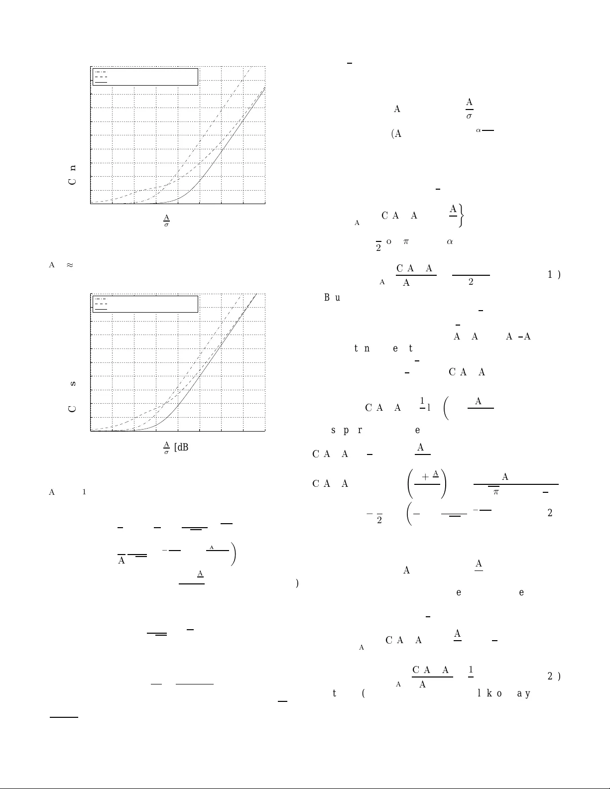
On the Capacity of Free-Space Optical Intensity Channels Amos Lapidoth ETH Zurich Zurich, Switzerland Email: lapidoth@isi.ee.eth z.ch Stefan M. Mose r National Chiao T ung Uni versity (NCTU) Hsinchu, T aiw an Email: stefan.moser@ieee.org Mich ` ele A. W igger ETH Zurich Zurich, Switzerland Email: wigger@isi.ee.ethz. ch Abstract — New upper and lower bounds are presented on the capacity of the fr ee-space optical intensity channel. Th is channel is characterized by inputs th at are nonnegative (representing the transmitted optical in tensity) and by outp uts that are corrupted by additive white Gaussian noise (because in fr ee space the distur - bances arise from many independen t sour ces). Due to battery and safety rea sons the inpu ts are simultaneously constrained in both their aver age and p eak power . For a fixed ratio of the a verage power to t he peak p ower th e difference between the upper and the lower bounds tend s to zero as th e a verage power tends to infinity , and the ratio of the upper and lower boun ds t ends to one as the a verage power tend s to zer o. The case where only an av erage-power constraint is imposed on the input is treated separately . In th is case, the d ifference of the u pper and lower b ound tend s to 0 as the a vera ge power ten ds to in finity , and their ratio tends to a constant as the po wer t ends to zero. I . I N T RO D U C T I O N W e con sider a chann el model for short optical co mmuni- cations in f ree space su ch as the com municatio n between a remote contr ol and a TV . W e assume a channe l m odel based on in tensity mod ulation where the signal is mo dulated o nto the optical intensity o f the emitted lig ht. Thus, the ch annel input i s propo rtional to the ligh t intensity and is therefo re nonnegative. W e further assume that th e receiver directly measures the incid ent op tical intensity of the incoming sign al, i.e. , it pro duces an electric al cu rrent at the ou tput which is propo rtional to the d etected in tensity . Since in amb ient light condition s the recei ved signal is disturbed by a high nu mber of indepen dent sourc es, we m odel the n oise as Gaussian. More- over , we assume th at the line-o f-sight compo nent is dominant and ignore any effects du e to multiple-path pr opagation like fading o r inter-symbol interfer ence. Optical com munication is restricted not only b y batter y power , but also for safety reasons by th e m aximum al- lowed pe ak power . W e therefore assume simultaneously two constraints: an av erage-p ower constraint E a nd a maximum allowed peak power A . The situatio n where only a p eak-power constraint is imposed co rrespon ds to E = A . The case of only an a verage-power constrain t is treated separately . In this work we study the channel cap acity of such an optical com munication channel an d present n ew upp er and lower bounds. The maximum gap between upper and lower bound n ev er exceeds 1 nat when the ratio of the average- power co nstraint to the pe ak-power constrain t is larger th an 0 . 03 o r whe n on ly the a verage power is constrained but n ot the peak power . Asympto tically when the av ailable average and peak po wer tend to infinity with th eir ratio h eld fixed, the upper and lower bo unds coincide, i.e. , their dif ference tends to 0. W e also present the asympto tic b ehavior of the channel capacity in the limit wh en th e power tends to 0. The channel model has be en studied before, e.g. , in [1] an d is described in detail in the following. The receiv ed signal is corrup ted by additive noise due to strong ambient light that causes high-intensity shot noise in the electrical output signal. In a first appr oximation this shot noise can b e assumed to be indepen dent of th e signal itself, and since the noise is caused by many in depend ent sources it is reasonable to mod el it as an indepen dent and identically distrib uted (IID) Gaussian process. Also, witho ut loss of generality we a ssume the no ise to be zero-mea n, since the receiver can always subtract or add any constant signal. Hence, the channel output Y k at time k , modeling a sample of the electrical o utput signal, is g iv en b y Y k = x k + Z k , (1) where x k ∈ R + 0 denotes the time- k channel inp ut an d represents a sample of the electrical inpu t cu rrent th at is propo rtional to the optical intensity and therefore no nnegative, and where the rando m proce ss { Z k } modeling the additive noise is gi ven by { Z k } ∼ II D N R  0 , σ 2  . (2) It is impo rtant to note tha t, unlike the input x k , the outp ut Y k may be negative since the noise introduced at the receiver can be negati ve. Since the op tical intensity is pro portion al to the optical power , in suc h a system th e instantan eous optical power is propo rtional to th e ele ctrical in put curren t [2]. This is in contrast to radio commun ication where usually the power is propo rtional to the squar e of the inp ut cu rrent. T herefor e, in addition to the imp licit nonnegativity co nstraint on the input, X k ≥ 0 , (3) we assume constraints both on the peak and the a verag e power , i.e. , Pr [ X k > A ] = 0 , (4) E [ X k ] ≤ E . (5) W e shall denote th e ratio b etween the average power an d the peak po wer by α , α , E A , (6) where we assume 0 < α ≤ 1 . Note that α = 1 correspond s to the case with only a peak-power constraint. Similarly , α ≪ 1 correspo nds to a dominant av erage-p ower con straint and only a very weak peak-p ower constraint. W e d enote the cap acity of the describe d channe l with peak-p ower constraint A and a verage-power co nstraint E by C ( A , E ) . The capacity is gi ven by [3] C ( A , E ) = s up I ( X ; Y ) (7) where I ( X ; Y ) stands for the mutual infor mation betwee n the channel input X and the chann el o utput Y , wh ere conditiona l on th e inpu t x the o utput Y is Gaussian ∼ N  x, σ 2  ; an d where th e supremu m is over all laws on X ≥ 0 satisfying Pr [ X ≥ A ] = 0 an d E [ X ] ≤ E . In the c ase of only an average-power constraint the capacity is denoted by C ( E ) . It is given a s in (7) except that the supremum is taken over all laws on X ≥ 0 satisfying E [ X ] ≤ E . The deriv ation of the upper bounds is based on a technique introdu ced in [ 4]. There a d ual expression of mutual inform a- tion is used to show that for any chann el law W ( ·|· ) and for an arbitra ry distribution R ( · ) over the chan nel output alph abet, the channel capacity is u pper-bound ed by C ≤ E Q ∗  D  W ( ·| X )   R ( · )  . (8) Here, D ( ·k · ) stands f or th e relative entropy [5, Ch. 2], and Q ∗ ( · ) den otes the capacity-ach ieving input distribution. For more details about this techniq ue and for a pro of of (8), see [4, Sec. V], [6, Ch. 2]. Th e challenge of using (8) lies in a clev er ch oice of the arbitra ry law R ( · ) that will lead to a good upper bound. Moreover , note that the bo und ( 8) still contain s an expectation over the (un known) capacity-achieving input distribution Q ∗ ( · ) . T o handle this expectation we will need to resort to some f urther boundin g like, e .g. , Jensen ’ s inequality [5, Ch. 2.6]. The deriv atio n of the firm lower bounds relies on the entropy power inequ ality [5, T h. 17.7.3]. The asymptotic resu lts at h igh power follow dir ectly by ev alu ation of the firm upper and lower b ound s. For the lo w power regime we intro duce an additional lower b ound which does not rely on the entropy p ower inequality . T his lower bound is obtained by choosing a binary input distribution, a choice which was inspired by [7], and by then evaluating the correspo nding mu tual infor mation. For the cases in volving a peak-p ower constraint we fu rther re sort to the r esults on the asymptotic expression of mu tual information for weak signals in [8]. The results of this p aper are partially based o n th e re sults in [9] and [6 , Ch. 3]. The remainder is structured as follows. In the subsequent section we state ou r resu lts an d in Section II I we gi ve a b rief outline of some o f the deri vations. I I . R E S U LT S W e start with an auxiliary lemma wh ich is based on the symmetry of the channel law and the con cavity of ch annel capacity in the input distribution. Lemma 1: Consider a p eak-power constra int A and an av erage-p ower constraint E such tha t α = A E > 1 2 . Th en th e optimal input distribution 1 in (7) has an average power equal to half the p eak power E Q ∗ [ X ] A = 1 2 , (9) irrespective o f α . I.e. , th e average-power constraint is inactiv e for all α ∈  1 2 , 1  , and in p articular C ( A , α A ) = C  A , A 2  , 1 2 < α ≤ 1 . (10) W e are now ready to state our results. W e will distinguish between three different cases: in the first two cases we im pose on the inp ut both an average- and a peak- power co nstraint: in the first case the average-to-peak power ratio α is restricted to lie in  0 , 1 2  , and in the second case it is restricted to lie in  1 2 , 1  . ( Note that by Lemma 1, 1 2 < α ≤ 1 represents the situatio n with an inactive average-power constraint.) In the third case we impose on th e inpu t an a verage p ower constraint only . In all thr ee cases we p resent firm u pper and lower bound s on the chan nel capacity . The d ifference of the upper and lower bound s tends to 0 when the a vailable a verag e and pea k power tend to in finity with the ir ratio he ld constant at α . Th us we ca n derive th e asymptotic capacity at hig h power exactly . W e also present the asy mptotics of capacity a t low power: for th e cases in volving a peak- power con straint we are able to state them exactly , an d for the case of only an av erage-p ower constraint we giv e the asymp totics up to a constant factor . A. B ounds on Channel Ca pacity with b oth an A ve rag e- and a P eak-P ower Constr aint ( 0 < α < 1 2 ) Theor em 2: If 0 < α < 1 2 , then C ( A , α A ) is lower - bound ed by C ( A , α A ) ≥ 1 2 log 1 + A 2 e 2 αµ ∗ 2 π eσ 2  1 − e − µ ∗ µ ∗  2 ! , (11) and upper-bound ed by eac h of th e two bou nds C ( A , α A ) ≤ 1 2 log  1 + α (1 − α ) A 2 σ 2  , (12) C ( A , α A ) ≤  1 − Q  δ + α A σ  − Q  δ + (1 − α ) A σ  · · log A σ · e µδ A − e − µ ( 1+ δ A ) √ 2 π µ  1 − 2 Q  δ σ  ! 1 It was shown in [1] that the optimal inp ut distr ibuti on in (7) is unique . −10 −5 0 5 10 15 20 25 30 0 0.5 1 1.5 2 2.5 3 3.5 4 4.5 5 P S f r a g r e p l a c e m e n t s A σ [dB] C [nats per c hannel use] lower bound ( 11), α =0 . 1 upper bo und (12), α =0 . 1 upper bd . (13), α =0 . 1 , u sing (16), (17) Fig. 1. Bounds of Theorem 2 for a choice of the avera ge-to-pea k power ratio α = 0 . 1 . T he free parameters ha ve been cho sen as suggested in (16 ) and (17). The maximum gap between upper and l owe r bound is 0.72 nats (for A /σ ≈ 11 . 8 dB). −10 −5 0 5 10 15 20 25 30 0 0.5 1 1.5 2 2.5 3 3.5 4 4.5 5 P S f r a g r e p l a c e m e n t s A σ [dB] C [nats per c hannel use] lower bound ( 11), α =0 . 4 upper bo und (12), α =0 . 4 upper bd . (13), α =0 . 4 , u sing (16), (17) Fig. 2. Bounds of Theorem 2 for a choice of the avera ge-to-pea k power ratio α = 0 . 4 . T he free parameters ha ve been cho sen as suggested in (16 ) and (17). The maximum gap between upper and l owe r bound is 0.56 nats (for A /σ ≈ 7 . 1 dB ). − 1 2 + Q  δ σ  + δ √ 2 π σ e − δ 2 2 σ 2 + σ A µ √ 2 π  e − δ 2 2 σ 2 − e − ( A + δ ) 2 2 σ 2  + µα 1 − 2 Q δ + A 2 σ !! . (13) Here Q ( · ) denote s the Q -fun ction defin ed by Q ( ξ ) , Z ∞ ξ 1 √ 2 π · e − t 2 2 t . , ∀ ξ ∈ R ; (14) µ > 0 and δ > 0 are fr ee parame ters; and µ ∗ is th e un ique solution of α = 1 µ ∗ − e − µ ∗ 1 − e − µ ∗ . (15) Note that µ ∗ is well-d efined as the function µ ∗ 7→ 1 µ ∗ − e − µ ∗ 1 − e − µ ∗ is strictly monotonica lly decreasing over (0 , ∞ ) and tends to 1 2 for µ ∗ ↓ 0 and to 0 f or µ ∗ ↑ ∞ . A subo ptimal but useful ch oice for the free parameters in the upper b ound (13) is δ = δ ( A ) , σ log  1 + A σ  , (16) µ = µ ( A , α ) , µ ∗  1 − e − α δ 2 2 σ 2  , (17) where µ ∗ is the solu tion to (1 5). F or this ch oice and fo r α = 0 . 1 and 0 . 4 the bou nds of Th eorem 2 are d epicted in Figu res 1 and 2. Theor em 3: If α lies in  0 , 1 2  , then χ ( α ) , lim A ↑∞  C ( A , α A ) − log A σ  = − 1 2 log 2 π e − (1 − α ) µ ∗ − log(1 − αµ ∗ ) (18) and lim A ↓ 0 C ( A , α A ) A 2 /σ 2 = α (1 − α ) 2 . (19) B. B ounds on Chann el Capa city with a Str ong P e ak-P ower and Inactive A verage-P ower Constr aint ( 1 2 ≤ α ≤ 1 ) By L emma 1 we have that fo r 1 2 < α ≤ 1 t he average- power constrain t is inactive and C ( A , α A ) = C ( A , 1 2 A ) . Thus we can obtain the results in this section by simply deri ving bound s for the case α = 1 2 . Theor em 4: If α ∈  1 2 , 1  , then C ( A , α A ) is lower -boun ded by C ( A , α A ) ≥ 1 2 log  1 + A 2 2 π eσ 2  , (20) and is upper-bounded by each of the two boun ds C ( A , α A ) ≤ 1 2 log  1 + A 2 4 σ 2  , (21) C ( A , α A ) ≤ 1 − 2 Q δ + A 2 σ !! log A + 2 δ σ √ 2 π  1 − 2 Q  δ σ  − 1 2 + Q  δ σ  + δ √ 2 π σ e − δ 2 2 σ 2 , (22) where δ > 0 is a free pa rameter . W e suboptimally choose δ = δ ( A ) , σ log  1 + A σ  . (23) For this choice the boun ds of Th eorem 4 are d epicted in Figure 3. Theor em 5: If α lies in  1 2 , 1  , then χ ( α ) , lim A ↑∞  C ( A , α A ) − lo g A σ  = − 1 2 log 2 π e (24) and lim A ↓ 0 C ( A , α A ) A 2 /σ 2 = 1 8 . (25) Note that (24) and (25) exhibit th e well-known asymptotic behavior of the capacity o f a Gaussian chann el under a peak - power constrain t o nly [3]. −20 −15 −10 −5 0 5 10 15 20 25 30 0 0.5 1 1.5 2 2.5 3 3.5 4 4.5 5 P S f r a g r e p l a c e m e n t s A σ [dB] C [nats per c hannel use] lower bound ( 20) upper bo und (21) upper bo und (22), using (23) Fig. 3. Bounds on the capac ity of the free -space optical intensi ty channel with av erage- and pe ak-po wer constraints for α ≥ 1 2 accordi ng to Theorem 4. T his include s t he case of onl y a peak- powe r constraint α = 1 . The free pa rameter has been cho sen as suggested in (23). The maximum ga p between upper and lo wer bou nd is 0.54 nats (for A /σ ≈ 7 dB). −30 −25 −20 −15 −10 −5 0 5 10 15 20 0 0.5 1 1.5 2 2.5 3 3.5 4 P S f r a g r e p l a c e m e n t s E σ [dB] C [nats per c hannel use] lower bound ( 26) upper bound (27), using (29), ( 30) upper bound (28), using (31), ( 32) Fig. 4. Bounds on the cap acity of the fre e-space optical intensity channel with only an av erage-po wer constrain t according to Theorem 6. The free paramete rs ha ve bee n cho sen as suggested in (29)–(32). The maximum gap betwee n upper and lower bound is 0.64 nats (for E /σ ≈ 1 . 8 dB) . C. Bounds o n Cha nnel Capa city with a n A verage-P ower Con- straint Finally , we con sider th e case with an a verage-power con- straint only . Theor em 6: In the a bsence of a peak- power co nstraint the channel capacity C ( E ) is lower-bounded by C ( E ) ≥ 1 2 log  1 + E 2 e 2 π σ 2  , (26) and is upper-bounded by each of the bo unds C ( E ) ≤ log  β e − δ 2 2 σ 2 + √ 2 π σ Q  δ σ  − log  √ 2 π σ  − δ E 2 σ 2 + δ 2 2 σ 2  1 − Q  δ σ  − E δ Q  δ σ  + 1 β  E + σ √ 2 π  , δ ≤ − σ √ e , (27) C ( E ) ≤ log  β e − δ 2 2 σ 2 + √ 2 π σ Q  δ σ  + 1 2 Q  δ σ  + δ 2 √ 2 π σ e − δ 2 2 σ 2 + δ 2 2 σ 2  1 − Q  δ + E σ  + 1 β  δ + E + σ √ 2 π e − δ 2 2 σ 2  − 1 2 log 2 π e σ 2 , δ ≥ 0 , ( 28) where β > 0 and δ are free parame ters. Note th at bo und (2 7) only hold s for δ ≤ − σ e − 1 2 , while bo und (28) only hold s for δ ≥ 0 . A subop timal but u seful choice for the f ree par ameters in b ound (27) is shown in ( 29) an d ( 30) an d fo r th e fr ee parameters in bo und (28) is shown in (31) and (32) at the top of the next page. For these cho ices, th e b ound s of Theorem 6 are depicted in Figu re 4. Theor em 7: In the ca se of on ly an average-power con - straint, χ E , lim E ↑∞  C ( E ) − log E σ  = 1 2 log e 2 π (33) and lim E ↓ 0 C ( E ) E σ p log σ E ≤ 2 , (34) lim E ↓ 0 C ( E ) E σ p log σ E ≥ 1 √ 2 . ( 35) Note that the asymptotic upper an d lo wer boun d at low SNR do no t coin cide in the sense that th eir ratio equ als 2 √ 2 instead of 1. H owe ver, they exhibit similar behavior . I I I . D E R I V AT I O N In the f ollowing we will ou tline the deriv ations of the firm lower and uppe r bo unds gi ven in the previous section. One easily find s a lower bou nd o n capacity by dro pping the maximization and choosing an arb itrary inp ut distribution Q ( · ) to c ompute the m utual info rmation between input and output. Howe ver , in o rder to get a tight bo und, this cho ice of Q ( · ) sho uld yield a mutual inform ation that is reason ably close to capacity . Such a cho ice is dif ficult to find an d might make the ev aluation of I ( X ; Y ) intr actable. T he reason for this is that even for relativ ely “easy” distributions Q ( · ) , the correspo nding d istribution on the chann el outpu t Y may be difficult to compu te, let alone h ( Y ) . W e circumvent th ese problem s by using the entropy power ineq uality [5, Th. 17. 7.3] to lower-bound h ( Y ) b y an expression that depend s o nly on h ( X ) . I.e. , we “tra nsfer” the prob lem of c omputing (o r bound ing) h ( Y ) to the in put side of the chann el, where it is much easier to choose an appro priate distribution tha t lead s to a tight lo wer bound on ch annel capacity: C = sup Q ( · ) I ( X ; Y ) (36) ≥ I ( X ; Y )   for a specific Q ( · ) (37) δ = δ ( E ) , − 2 σ r log σ E , for E σ ≤ e − 1 4 e ≈ − 0 . 4 dB , (29) β = β ( E ) , 1 2  E + σ √ 2 π  + 1 2 s  E + σ √ 2 π  2 + 4  E + σ √ 2 π  √ 2 π σ e δ 2 2 σ 2 Q  δ σ  , (30) δ = δ ( E ) , σ log  1 + E σ  , (31) β = β ( E ) , 1 2  δ + E + σ √ 2 π e − δ 2 2 σ 2  + 1 2 s  δ + E + σ √ 2 π e − δ 2 2 σ 2  2 + 4  δ + E + σ √ 2 π e − δ 2 2 σ 2  √ 2 π σ e δ 2 2 σ 2 Q  δ σ  . (3 2) =  h ( Y ) − h ( Y | X )    for a specific Q ( · ) (38) = h ( X + Z )   for a specific Q ( · ) − h ( Z ) (39) ≥ 1 2 log  e 2 h ( X ) + e 2 h ( Z )      for a specific Q ( · ) − h ( Z ) (40) = 1 2 log  1 + e 2 h ( X ) 2 π eσ 2      for a specific Q ( · ) (41) where the inequality in (40) follows from th e en tropy power inequality . T o make th is lower bound as tigh t as p ossible we will ch oose a distribution Q ( · ) that m aximizes d ifferential entropy under th e gi ven co nstraints [ 5, Ch. 12]. The deriv atio n of the upper bounds in Section II are based on the dua lity ap proach (8). Hence, we n eed to specify a distribution R ( · ) a nd e valuate the relative entropy in (8). W e have chosen output distributions R ( · ) with the following densities. F or (12) we choose R ′ ( y ) , 1 p 2 π ( σ 2 + E ( A − E )) e − ( y −E ) 2 2 σ 2 +2 E ( A −E ) ; (42) for (13) we ch oose R ′ ( y ) ,              1 √ 2 π σ e − y 2 2 σ 2 , y < − δ, 1 A · µ ( 1 − 2 Q ( δ σ )) e µδ A − e − µ ( 1+ δ A ) e − µy A , − δ ≤ y ≤ A + δ, 1 √ 2 π σ e − ( y − A ) 2 2 σ 2 , y > A + δ, (43) where δ > 0 and µ > 0 are free parameter s; fo r (21) we choose R ′ ( y ) , 1 r 2 π  σ 2 + A 2 4  e − ( y − A 2 ) 2 2 σ 2 + A 2 2 ; (44) for (22) we ch oose R ′ ( y ) ,            1 √ 2 π σ e − y 2 2 σ 2 , y < − δ, 1 − 2 Q ( δ σ ) A +2 δ , − δ ≤ y ≤ A + δ, 1 √ 2 π σ e − ( y − A ) 2 2 σ 2 , y > A + δ, (45) where δ > 0 is a free parameter; and for (27) and (2 8) we choose R ′ ( y ) ,        1 β e − δ 2 2 σ 2 + √ 2 π σ Q ( δ σ ) e − y 2 2 σ 2 , y < − δ, 1 β e − δ 2 2 σ 2 + √ 2 π σ Q ( δ σ ) e − δ 2 2 σ 2 e − y + δ β , y ≥ − δ, (46) where δ ∈ R and β > 0 a re fr ee parameter s. In the d eriv a tion of (28) we then restrict δ to b e nonn egati ve, wh ile in the deriv ation of (2 7) we restrict δ ≤ − σ e − 1 2 . A C K N O W L E D G M E N T S The autho rs would like to thank Ding -Jie Lin for fr uitful discussions. The work of S. M. Moser was suppor ted in part by the E TH under TH-23 0 2-2. R E F E R E N C E S [1] T . H. Chan, S. Hrani lovic , and F . R. Kschischa ng, “Capa city-ac hie ving probabil ity measure for conditional ly Gaussian channel s with bounded inputs, ” IE EE T rans. Inf. Theory , vol. 51, no. 6, pp. 2073–2088, Jun. 2005. [2] J. M. Kahn and J. R. Barry , “W ireless infrared communicat ions, ” Pr oc. IEEE , vol. 85, no. 2, pp. 265–298, Feb. 1997. [3] C. E . Shannon, “ A mathematical the ory of communication, ” B ell System T echn. J. , vol. 27, pp. 379 –423 and 623–656, Jul. and Oct. 1948. [4] A. Lapidoth and S. M. Moser , “Capacity bounds via duality with applic ations to multiple-an tenna systems on flat fading channe ls, ” IEEE T rans. Inf. Theory , v ol. 49, no. 10, pp. 2426–2467, Oct. 2003. [5] T . M. Cover and J. A. Thomas, Ele ments of Informati on Theory , 2nd ed. John W ile y & Sons, 2006. [6] S. M. Moser, “Duali ty-based bounds on channe l capacit y , ” Ph.D. dissertat ion, Swiss Fed. Inst. of T echnol. (ETH), Z urich, Oct. 2004, Diss. ETH No. 15769. [Online]. A vaila ble: http: //moser .cm.nctu.edu.tw/ [7] J. G. Smith, “The information capacity of amplitude and va riance- constrai ned scalar Gaussian channel s, ” Inform. Con tr ., vol. 18, pp. 203– 219, 1971. [8] V . V . Prelo v and E . C. van der Meulen, “ An asympt otic expression for the information and capacit y of a multidimensi onal channel with weak input signals, ” IEEE T rans. Inf . Theory , vol. 39, no. 5, pp. 1728–1 735, Sep. 1993. [9] M. A. W igger , “Bounds on the capacit y of free-space opti cal intensit y channe ls, ” Master’ s thesis, Signal and Inf. Proc. L ab ., ETH Zurich, Switzerl and, Mar . 2003, supervi sed by Prof. Dr . Amos Lapidoth.