Some conjectures about q-Fibonacci polynomials

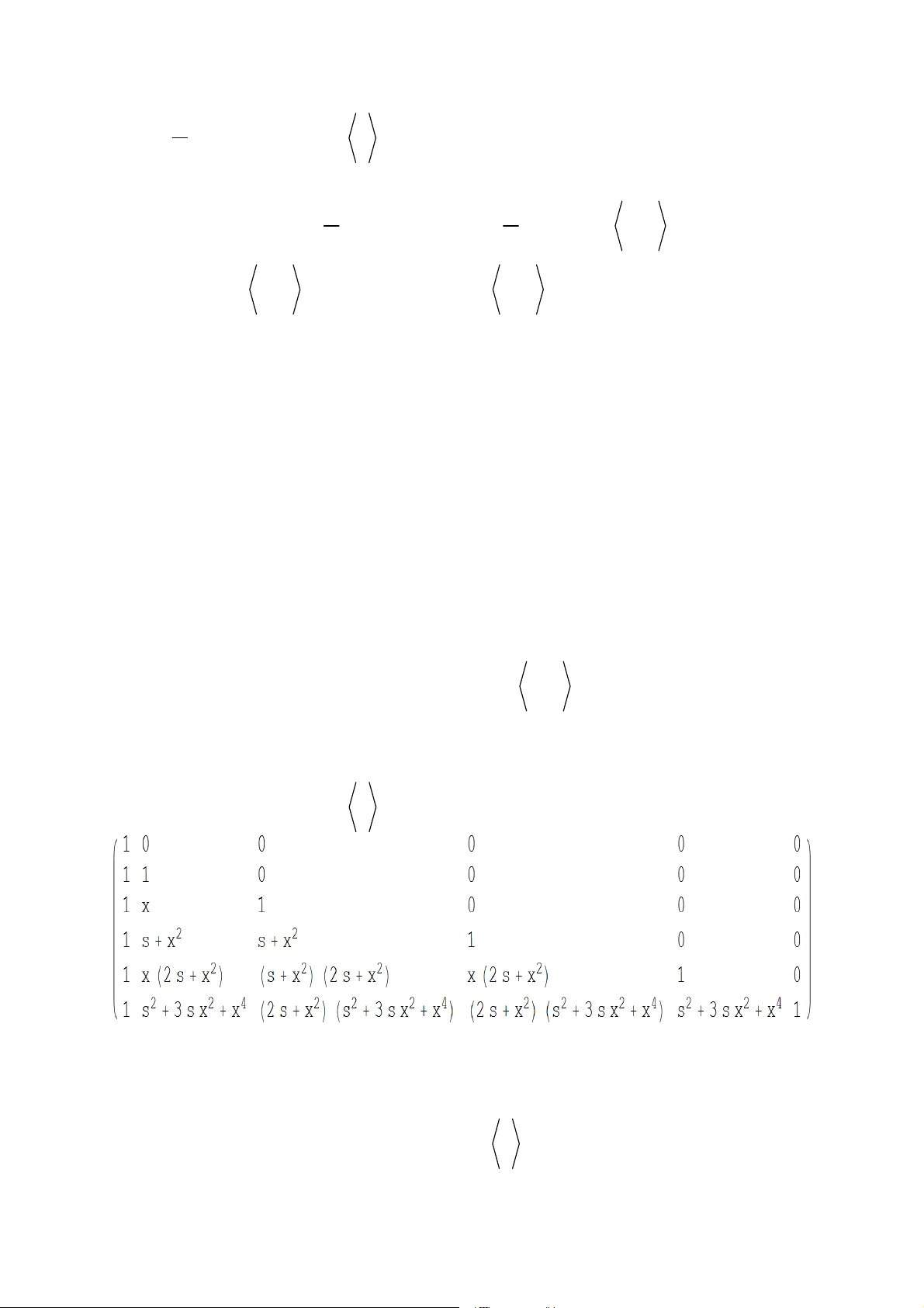
1 Some conjectures about q- Fibonacci poly nomials Johann Cigler Fakultät für Mathematik Universität Wien A-1090 Wien, Nordbergstraße 15 Johann Cigler@univie.ac.at Abstract In this paper we state some conjectures about q − Fibonacci polynomials which for 1 q = reduce to well-known results about Fibon acci numbers and Fibonacci polynom ials. 1. Introduction The Fibonacci numbers n F are defined by the recurrence relation 12 nn n FF F − − = + (1.1) with initial values 0 0 F = and 1 1. F = The powers k n F , 1 , 2, 3 , , k = " satisfy the recurrence relation 1 1 2 0 1 (1 ) 0 , j k k nj j k F j + ⎛⎞ + ⎜⎟ ⎝⎠ − = + − = ∑ (1.2) where 1 0 1 k ni i k i i F n k F − − = = = ∏ ∏ is a so called fibonomial coefficient. E.g. the squares of the Fibonacc i numbers satisfy the recurrence 22 2 2 12 3 22 0 . nn n n FF F F −− − − −+ = The triangle of Fibonomial co efficients ( see A010048 or A055870 in the On-Line Encyclopedia of Integer Sequences [8] ) begins with 1 1 1 1 1 1 1 2 2 1 1 3 6 3 1 1 5 15 15 5 1 The Fibonacci polynomials ( , ) n Fx s are defined by the recurrence relation 12 (,) (,) (,) nn n Fx s x F x s s F x s −− = + (1.3) 2 with initial values 0 (,) 0 Fx s = and 1 (,) 1 . Fx s = The first terms of this sequence are 23 4 2 2 0, 1 , , , 2 , 3 , xx sx s xx s x s ++ + + " . The powers ( , ) k n Fx s , 1 , 2, 3 , , k = " satisfy the recurrence relation 1 1 22 0 1 (1 ) ( , ) ( , ) 0 , jj k k nj j k sx s F x s j + ⎛⎞ ⎛ ⎞ + ⎜⎟ ⎜ ⎟ ⎝⎠ ⎝ ⎠ − = + −= ∑ (1.4) where the polynomial fibonomial co efficients are defined by 1 0 1 (,) (,) . (,) k ni i k i i Fx s n xs k Fx s − − = = = ∏ ∏ (1.5) E.g. for 2 k = we get the recurrence relation 22 2 2 2 3 2 12 3 (,) ( ) (,) ( ) (,) (,) 0 . nn n n F xs x s F xs s x sF xs s F xs −− − −+ − + + = The simplest proof of these facts depends on the Binet formula (,) , nn n Fx s α β α β − = − (1.6) where 22 44 ,. 22 x xs x xs αβ ++ −+ == (1.7) From (1.6) it is clear tha t (,) k n Fx s is a linear combination of () kj n j n α β − , 0 j k ≤≤ . Let U be the shift operator ( ) ( 1 ). Uh n h n =− The sequences ( ) () 0 kj n j n n αβ − ≥ satisfy the recurrence relation ( ) ( ) () 10 . kj j kj n j n U αβ α β −− −= Since the operators 1 kj j U α β − − commute we get 0 (1 ) ( , ) 0 . n kj j k n j UF x s αβ − = ⎛⎞ − = ⎜⎟ ⎝⎠ ∏ (1.8) As has been observed by L. Car litz [2] we can now apply the q − binomial theorem (cf. e.g. [4]) 1 2 00 (1 ) ( 1) . k nn jk k jk n qx q x k ⎛⎞ − ⎜⎟ ⎝⎠ == ⎡ ⎤ −= − ⎢ ⎥ ⎣ ⎦ ∏∑ (1.9) Here 11 2 (1 ) (1 ) (1 ) () (1 ) (1 ) (1 ) nn n k k nn qq q q kk qq q −− − ⎡⎤ ⎡⎤ −− − == ⎢⎥ ⎢⎥ −− − ⎣⎦ ⎣⎦ " " denotes a q − binomial coefficient. 3 For q β α = we get 2 (,) . kn k nn x s kk α − ⎡⎤ = ⎢⎥ ⎣⎦ This implies () 2 2 (1 ) 00 0 1 22 2 00 1 (1 ) (1 ( ) ) ( 1) ( , ) 11 ( 1 ) (,) ( 1 ) (,) . j j kk k kj j k j j k j k j j jj j jj j kk jj j jj k UU x s U j kk xs U s xs U jj ββ αβ α α α αα αβ ⎛⎞ ⎜⎟ ⎝⎠ − −+ == = + ⎛⎞ ⎛ ⎞ ⎛⎞ ⎜⎟ ⎜ ⎟ ⎜⎟ ⎝⎠ ⎝ ⎠ ⎝⎠ == + ⎛⎞ ⎛⎞ −= − = − ⎜⎟ ⎜⎟ ⎝⎠ ⎝⎠ ++ =− =− ∏∏ ∑ ∑∑ By applying this operator to ( , ) k n Fx s we get (1.4). The Lucas polynomials (,) nn n Lx s α β = + (1.10) satisfy the sam e recurrence 12 (,) (,) (,) nn n Lx s x L x s s L x s −− = + with initial values 0 (,) 2 Lx s = and 1 (,) Lx s x = . Therefore for 2 jk < the coefficients of the product ( ) 22 2 2 2 () () ( ) ( ) ( ) ( , ) ( ) kj j j kj j k j k j k j k kj zz z z z s L x s z s αβ α β α β α β α β −− − − − −− = − + + = − − + − are polynomials in x and s with integer coefficients. The same is true if 2 . kj = In this case we have 2 () ( ) . jj j j j zz z s αβ α β − −= − = − − This implies that the coef ficients of 1 22 1 00 1 () ( 1 ) ( , ) jj kk kj j k j jj k zs x s z j αβ + ⎛⎞ ⎛ ⎞ ⎜⎟ ⎜ ⎟ −+ − ⎝⎠ ⎝ ⎠ == + −= − ∏∑ (1.11) are polynomials in x and s with integer coefficients. The matrix of the polynom ials (,) k x s j begins with Remark The polynomial 1 22 1 10 () ( 1 ) ( , ) jj nn jn j n j jj n zs x s z j αβ + ⎛⎞ ⎛ ⎞ ⎜⎟ ⎜ ⎟ −− − ⎝⎠ ⎝ ⎠ == −= − ∏∑ also appears as the characteristic polynomial () det ( ) n zI a n − of the matrix 4 1 ,1 1 () . n ij n nj ij i an x s nj +−− − = − ⎛⎞ ⎛⎞ = ⎜⎟ ⎜⎟ − ⎝⎠ ⎝⎠ For the special case 1 x s = = this conjecture by V.E. Hogga tt has been proved by L. Carlitz [2]. H. Prodinger [7] has given a simple proof that the eigenvectors (, ) un j which belong to the eigenvalues 1 jn j j λ αβ −− = , 1 j n ≤≤ , are (, 1 , ) (, 2 , ) (, ) (, , ) un j un j un j unn j ⎛⎞ ⎜⎟ ⎜⎟ = ⎜⎟ ⎜⎟ ⎝⎠ # with 21 1 1 (, , ) ( ) 1 j ik ki k in i un i j s kj k α −− − = −− ⎛⎞ ⎛ ⎞ =− ⎜⎟ ⎜ ⎟ −− ⎝⎠ ⎝ ⎠ ∑ . 2. Recurrence relations for powe rs of q-Fibonacci polynomials The (Carlitz-) q − Fibonacci polynomials ( , , ) f nx s are defined by 2 (, ,) ( 1 , ,) ( 2 , ,) n f n x s x fn x s q s fn x s − =− + − (2.1) with initial values ( 0 , , ) 0 , ( 1 , , ) 1 fx s f x s == (cf. [3],[5]). The first values are 0, 1, x, q s+x 2 , q s x+q 2 s x+x 3 , q 4 s 2 +q s x 2 +q 2 s x 2 +q 3 s x 2 +x 4 . An explicit expression is 2 12 1 1 (, ,) . kn k k kn nk f nx s q x s k −− ≤− −− ⎡⎤ = ⎢⎥ ⎣⎦ ∑ (2.2) If we change 1 q q → and then 1 n sq s − → we get 1 (, , ) (, ,) ( , , ) . kn f nk x q s f nk x qs f n x s −− −→ − → Therefore each identity ( , , ,( , , ) ,( 1 , , ) ,( 2 , , ) , ) 0 g x s q fn x s fn x s fn x s − −= " (2.3) is equivalent with the iden tity 11 2 ( , , ,( , , ) ,( 1 , , ) ,( 2 , , ) , ) 0 . n gx q s q f n x s f n x q s f n x q s −− − −= " (2.4) 5 As a special case we get the well-known fact that (2.1) is equivalent with 2 (, , ) ( 1 , , ) ( 2 , , ) . f nx s x f n x q s q s f n x q s =− + − (2.5) The definition of the q − Fibonacci polynomials can be extended to all integers such that the recurrence (2.1) remains true. We then get (cf. [5]) 1 2 1 (, , ) (, , ) ( 1 ) . n n n n f nx q s fn x s q s + ⎛⎞ − ⎜⎟ − ⎝⎠ −= − (2.6) We are now looking for a q − analog of (1.4). Computer experiments suggest the following Conjecture 1 Let 1 11 (, , ) (,, ) . (, , ) (, , ) k i jk j ji j ii fi x s k xsq j f ix q s f ix q s = − − == = ∏ ∏∏ (2.7) Then the following recurr ence relation holds for all n ∈ ] : 1 (1 ) ( 21 ) 1 22 6 0 1 (1 ) ( , , ) ( , , ) 0 . jj jj j k jk j k sq x s q f n j x q s j + ⎛⎞ ⎛ ⎞ −− + ⎜⎟ ⎜ ⎟ ⎝⎠ ⎝ ⎠ = + −− = ∑ (2.8) This relation is equivalent to 1 (1 ) ( 21 ) 1 (1 ) 22 2 6 0 ( 1 ) ( 1 , ,) ( , ,) 0 jj j jj j k n k j s q fibo k x s f n j x s + ⎛ ⎞ ⎛⎞ ⎛⎞ −− + −− ⎜ ⎟ ⎜⎟ ⎜⎟ ⎝ ⎠ ⎝⎠ ⎝⎠ = −+ − = ∑ (2.9) with 11 1 11 (, , ) 1 (1 , , ) ( , , ) . (, , ) (, , ) k ni n i jk j nj n ij ii fi x q s k fibo k x s x q s q j f ix q s f ix q s − −− = − −− − == + += = ∏ ∏∏ (2.10) This conjecture is trivially true for 1. k = It should be noted that (, , ) f nx s is a q − holonomic sequence of polynomials. A sequence ( ( )) an is q − holonomic if there exist nontrivial polynomials 0 ,, r p p " such that 01 () ( ) () ( 1 ) () ( )0 . nn n r p q an p q an p q an r +− + + − = " I f (() ) an is q − holonomic then for each k ∈ ` the sequence ( ) () k an also is q − holonomic. Therefore it is clear that ( ) (, , ) k f nx s has a q − holonomic recurrence. With the help of the Mathematica package qGeneratingFunction by Christoph K outschan (RISC Linz) I have computed recursion (2.9) for sm all values of . k 6 For 2 k = (2.9) reduces to 22 2 2 2 2 2 2 3 8 3 2 (, ,) ( ) ( 1 , , ) ( ) ( 2 , ,) ( 3 , ,) 0 nn n n fn x s x q s fn x s q s x q sfn x s q s fn x s −− − − −+ − − + − + − = and (2.8) to 22 2 2 2 2 53 3 2 (, , ) ( ) ( 1 , , ) ( ) ( 2 , , ) (3 , , )0 . f n x s x qs f n x qs qs x qs f n x q s qs f n x qs −+ − − + − +− = (2.11) To prove this we use the q − Euler-Cassini formula (cf. [5], Cor. 2.2, see also (3.7)) 2 1 ( 1 ,, ) ( ,, ) ( ,, ) ( 1 ,, ) ( 1 ) ( ,, ) . k kk k f k x q s f n kx s f kx s f n k x q s q s f n x q s ⎛⎞ ⎜⎟ − ⎝⎠ −+ − + − = − (2.12) For each k ∈ ` it gives a representation of ( , , ) k f nk x q s − as a linear combination of (, , ) f nx s and ( 1 , , ) : f nx q s − () 1 ( ,, ) ( 1 ,, ) ( ,, ) ( ,, ) ( 1 ,, ) () k f n k x q s fk x q sfn x s fk x sfn x q s vk −= − − − (2.13) with 2 1 () ( 1 ) . k kk vk q s ⎛⎞ ⎜⎟ − ⎝⎠ =− If we set ( , , ) , ( 1 , , ) f nx s a f n x q s b =− = we get () 2 1 (2 , , ) f nx q s a x b qs −= − and () 32 32 1 (3 , , ) ( ) . f nx q s x a x q s b qs − −= − + Therefore (2.11) becomes () 25 3 2 22 2 2 2 23 2 2 () () ( ) () 0 . () ( ) qs x qs q s a x qs b a xb xa x qs b qs q s + −+ − − + −+ = − This is evident since all the coefficients of 22 ,, aa b b vanish. In the same way I have verified the conjecture for other sm all values of . k 3. Recurrence relations for subsequences In the classical case 1 q = formula (1.4) can be generalized to () 1 22 () 0 1 (1 ) ( , , ) (, ) 0 jj k j k nj j k sx s F x s j ⎛⎞ ⎛⎞ + + ⎜⎟ ⎜⎟ ⎝⎠ ⎝⎠ − = + −= ∑ AA A A (3.1) with () 1 () 0 1 (,) ,, . (,) j ki i j i i Fx s k xs j Fx s − − = = = ∏ ∏ A A A (3.2) This follows from the same argum ent as above by changing , α αβ β →→ AA . An analogous formula seems to hold in the general case. 7 Conjecture 2 For all integers 1 k ≥ and 1 ≥ A the following recurrence holds for all : n ∈ ] (4 1 ) 3 1 2 2 6 0 1 (1 ) ( , , , ) ( ( ) , , ) 0 j j j k j jk j k qs x s q f n j x q s j ⎛⎞ ⎛⎞ ⎜⎟ +− + + ⎝⎠ ⎜⎟ ⎝⎠ = + ⎛⎞ −− = ⎜⎟ ⎝⎠ ∑ A A A A AA (3.3) with 1 () 11 (, , ) (, , , ) . (, , ) (, , ) m i jm j ji j ii fi x s m xsq j f ix q s f ix q s = − − == = ∏ ∏∏ AA A A AA (3.4) Let us first consider the case 1. k = Here (3.3) reduces to (3 1 ) 2 2 (2 , , ) ( , , ) (, , ) ( ( 1 ) , , )( 1 ) ( ( 2 ) , , ) 0 . (, , ) (, , ) fx s f x s fn x s f n x q s q s f n x q s fx q s fx q s − −− + − − = AA AA A A A A AA AA A AA (3.5) For 1 q = this is the well-known recurren ce (1 ) ( 2 ) (,) (,) (,) ( ) (,) 0 . nn n Fx s L x s F x s s F x s −− −+ − = A AA A A (3.6) For in this case we have 22 2 (,) (,) . (,) Fx s Lx s Fx s αβ αβ αβ − == + = − AA AA A A AA A In order to prove (3.5) we prove the slightly m ore general formula (( 2 ) 1) 1( 1 ) 2 (( 1 ) , , ) ( ( 1 ) , , ) d e t ( 1 ) ,, ) ( ,, ) . ( , ,) ( , ,) ( mm mm m fN m x s f m x s sq x s f N x q s fN m x q s f m x q s f +− −+ ++ + ⎛⎞ =− ⎜⎟ + ⎝⎠ AA AA A AA AA A AA (3.7) From 2( 1 ) (, , ) ( 1 , , ) ( 2 , , ) Nm f Nm x q s x f Nm x q s q s f Nm x q s −+ + += + − + + − AA A A AA A and 2( 1 ) ( ( 1 ) ,, ) ( ( 1 ) 1 ,, ) ( ( 1 ) 2 ,, ) Nm f Nm x s x f Nm x s q s f Nm x s −+ + + + = + +− + + +− A AA A we see that (( 1 ) , , ) ( ( 1 ) , , ) () : d e t (, , ) ( , , ) f N m xs f m xs gN f Nm x q s f m x q s ++ + ⎛⎞ = ⎜⎟ + ⎝⎠ AA AA AA satisfies 2( 1 ) () ( 1 ) ( 2 ) Nm gN x gN q s gN −+ + =− + − A and ( 0) 0. g = Therefore (1 ) () (, , ) m gN c f N x q s + = A for some constant . c To compute c we set . Nm = − A This gives (1 ) () ( , , ) ( , , ) (, , ) m g m f x s f mx q s c f mx q s + −= = − AA AA A A or (( 2 ) 1) 2 () ( , , ) . mm m cs q f x s +− =− − AA A A Therefore we get (3.7). Remark For 1 , 1 km k =→ − (3.7) gives the q − Euler-Cassini formula (2.12). 8 If we let n →∞ in (2.2) with 1 x = we get 2 2 0 () . (1 ) (1 ) (1 ) k k k k q Fs s qq q ≥ = −− − ∑ " (3.8) If we let n →∞ in the q − Euler-Cassini formula we get 2 1 (1 , 1 , ) ( ) ( , 1 , ) ( ) ( 1 ) () . k kk k f kq s F s f k s F q s q s F q s ⎛⎞ ⎜⎟ − ⎝⎠ −− = − The special case 1 s = is closely connected with the famous Rogers-Ramanujan identities (cf. [1]). For 2 k = formula (3.3) reduce s to 22 (3 1 ) 22 2 2 (13 3 ) 13 2 2 (3 , , ) (2 , , ) (, , ) ( , , ) (, , ) ( 2, , ) ( 3 ,, ) ( ,, ) (1 ) ( 2 , , ) (, , ) (, , ) (, , ) ( 2, , ) (1 ) ( (, , ) ( 2 , , ) fx s f x s fn x s fn x q s fx q s f x q s fx s f x s qs f n x q s fx q s fx q s fx s f x s sq f n fx q s f x q s − − − −− +− − +− − A AA AA AA A AA AA AA AA AA AA A AA AA AA AA AA A AA 32 3, , ). x qs A A (3.9) This can be proved in the same way as in th e special case 1 = A by using (3.5) in order to reduce all expressions 2 (, , ) j f nj x q s − A AA to 3 (3 , , ) af n x q s =− A AA and 2 (2 , , ) . bf n x q s =− A AA For other small values of k formula (3.3) can be verified in the same way. But I did not find a proof for all . k 4. A generalization of Cassini’s identity A well-known formula for Fibonacci num bers is Cassini’s id entity 1 1 1 det ( 1 ) . nn n nn FF FF − − − ⎛⎞ =− ⎜⎟ ⎝⎠ (4.1) This can be generalized in the following way: Let 2 (, ,) (,) (,) (,) . n Fac n s F x s F x s F x s = AA A A" (4.2) Then () 11 1 1 () () 2 22 3 2 ,0 00 det ( , ) ( 1 ) ( , ,1 ) . kk k kk nk nk k k ni j ij j k Fx s s F a c k j s ++ + ⎛⎞ ⎛⎞ ⎛⎞ − −− + ⎜⎟ ⎜⎟ ⎜⎟ ⎝⎠ ⎝⎠ ⎝⎠ +− = == ⎛⎞ =− − ⎜⎟ ⎝⎠ ∏∏ A A (4.3) As a special case we get 9 22 2 12 22 2 11 22 2 21 det 2( 1 ) . nn n n nn n nn n FF F FF F FF F −− +− ++ ⎛⎞ ⎜⎟ =− ⎜⎟ ⎜⎟ ⎝⎠ To prove this we use again Binet’s formula: () () () () 2 () ( ) () ,0 0 1 det ( , ) det det ( 1 ) . k ni j ni j k k k n ijk n ij ni j k kk ij k Fx s αβ αβ αβ αβ +− +− +− − +− +− + = = ⎛⎞ ⎛⎞ − ⎛⎞ ⎛⎞ ⎜⎟ ⎜⎟ == − ⎜⎟ ⎜⎟ ⎜⎟ ⎜⎟ − ⎝⎠ − ⎝⎠ ⎝⎠ ⎝⎠ ∑ AA A A A Let now () ( ) () (1) ( ) (1) () ( ) () (, ) . njk nj nj k nj nk j k nk j zj αβ αβ αβ −− − +− − +− +− − +− ⎛⎞ ⎜⎟ ⎜⎟ = ⎜⎟ ⎜⎟ ⎝⎠ AA AA AA A # Then we get () 1 () ( ) () 2 00 d e t ( 1 ) ( 1 ) d e t ( 0 ,( 0 ) ) , ( 1 ,( 1 ) ) , ( ,( ) ) s g n ( ) , k kk ni j k ni j kk zz z k k π α βπ π π π + ⎢⎥ ⎢⎥ +− − +− ⎣⎦ == ⎛⎞ ⎛⎞ ⎛⎞ −= − ⎜⎟ ⎜⎟ ⎜⎟ ⎝⎠ ⎝⎠ ⎝⎠ ∑∏ ∑ AA A AA " AA where the sum is over all permutations π of { } 0, , k " . This implies () () 1 () ( ( ) ) () ( ) 2 (1 ) ,0 00 1 det ( , ) ( 1 ) sgn( ) k kk k k ni k i ni i ni j kk ij i k Fx s d ππ π πα β αβ + ⎢⎥ ⎢⎥ −− − ⎣⎦ +− + = == ⎛⎞ ⎛⎞ ⎛⎞ =− ⎜⎟ ⎜⎟ ⎜⎟ ⎜⎟ − ⎝⎠ ⎝⎠ ⎝⎠ ∏∑ ∏ A A with ( ) ( ) det . i kj j d αβ − = By the formula for Vandermonde’s determinant we get () ( ) () ( ) ( ) ( ) () ( ) () () ( ) () () () () 1 2 12 2 1 2 2 11 11 22 2 2 22 1 1 11 1 23 2 det ( 1 ) (1 ) ( ) (1 ) ( ) k i kj j k k k k k k k k kk k k kk k k kk k k kk k d s αβ α α β α αβ α β α β αβ αβ β α β β α βα β α β α β α β α β α β αβ + ⎛⎞ ⎜⎟ −− − − − ⎝⎠ −− +− ⎛⎞ ⎛ ⎞ ⎛⎞ ⎛ ⎞ ++ ⎜⎟ ⎜ ⎟ ⎜⎟ ⎜ ⎟ −− ⎝⎠ ⎝ ⎠ ⎝⎠ ⎝ ⎠ ++ ⎛⎞ ⎛⎞ + ⎛⎞ ⎜⎟ ⎜⎟ ⎜ ⎝⎠ ⎝⎠ ⎝⎠ == − − − − − −− = − − − − −−− =− − − " " "" "" " 1 0 (, , 1 ) . k j Fac k j s − ⎟ = − ∏ The sum () ( ( ) ) () ( ) 0 sgn( ) k ni k i ni i i ππ π πα β −− − = ∑∏ equals , det( ) ij c with ( ) , ni kj j ij c αβ − − = , which gives () , 0 det( ) . k nk kj j ij j cd αβ − − = = ∏ Therefore we finally get 10 () () () () () 1 1 2 2 2 (1 ) ,0 00 1 () 2 22 (1 ) 0 1 () 2 (1 ) 0 1 det ( , ) ( 1 ) 1 () 1 (1 ) k k kk k nk k kj j ni j kk ij j k k nk kk k k nk kk k Fx s d k ds d k αβ αβ αβ αβ + ⎛⎞ + ⎢⎥ + ⎜⎟ − ⎢⎥ − ⎣⎦ ⎝⎠ +− + = == + ⎛⎞ − ⎜⎟ ⎝⎠ + = + ⎛⎞ − ⎜⎟ ⎝⎠ + = ⎛⎞ ⎛⎞ =− ⎜⎟ ⎜⎟ ⎜⎟ − ⎝⎠ ⎝⎠ ⎛⎞ ⎛⎞ =− ⎜⎟ ⎜⎟ ⎜⎟ − ⎝⎠ ⎝⎠ ⎛⎞ ⎛⎞ =− ⎜⎟ ⎜⎟ ⎜⎟ − ⎝⎠ ⎝⎠ ∏∏ ∏ ∏ A A A A A A () 11 11 () 2 2 23 2 2 0 (, , 1 ) . kk kk nk j sF a c k j s αβ ++ ⎛⎞ ⎛⎞ +− ⎛⎞ −+ ⎜⎟ ⎜⎟ ⎜⎟ ⎝⎠ ⎝⎠ ⎝⎠ = −− ∏ A q − analog of Cassini’s identity is 2 2 2 2 (, , ) ( 1 , , ) (,) d e t (1 , , ) ( , , ) ( 1 ,, ) ( 2 ,, ) ( 1 ,, ) det ( ,, ) ( 1 ,, ) ( ,, ) (2 , , ) ( 1 , , ) det ( ( 1 ,, ) ( ,, ) fn x s fn x q s dn s fn x s fn x q s x f n xq s q s f n xqs f n xq s xf n x qs qsf n x q s f n x qs qsf n x q s f n x qs qsd qsf n x q s f n x qs − ⎛⎞ = ⎜⎟ + ⎝⎠ ⎛⎞ −+ − − = ⎜⎟ +− ⎝⎠ ⎛⎞ −− == − ⎜⎟ − ⎝⎠ 1, ) nq s − which gives 2 11 (,) ( 1 ) . n nn dn s q s ⎛⎞ ⎜⎟ −− ⎝⎠ =− This identity can be generalized to 22 2 2 (1 ) ( 3 4 ) 22 2 2 2 3 4 2 22 2 2 (, , ) ( 1 , , ) ( 2 , , ) det ( 1 , , ) ( , , ) ( 1 , , ) 2( 1 ) . (2 , , ) ( 1 , , ) ( , , ) nn nn fn x s fn x q s fn x q s fn x s fn x q s fn x q s x s q fn x s fn x q s fn x q s +− − ⎛⎞ −− ⎜⎟ +− = − ⎜⎟ ⎜⎟ ++ ⎝⎠ (4.4) For 2 n = this can be verified by computation. In the general case we have using (2.11) 22 2 2 22 2 2 22 2 2 53 3 2 2 2 2 53 3 2 2 (, , ) ( 1 , , ) ( 2 , , ) ( , ) d e t ( 1 ,, ) ( ,, ) ( 1 ,, ) (2 , , ) ( 1 , , ) ( , , ) (3 , , ) ( 1 , , ) (2 , ,) det ( 2, , ) ( , , ) ( 1 fn x s fn x q s fn x q s dn s f n x s f n x q s f n x q s fn x s fn x q s fn x q s q s fn x q s fn x q s fn x q s q s fn x q s fn x q s fn ⎛⎞ −− ⎜⎟ =+ − ⎜⎟ ⎜⎟ ++ ⎝⎠ −− − =− − 22 5 3 53 3 2 2 2 2 ,, ) ( 1 , ) . (1 , ,) (1 , , ) ( , , ) x qs q s d n q s q s fn x q s fn x q s fn x q s ⎛⎞ ⎜⎟ =− − ⎜⎟ ⎜⎟ −+ ⎝⎠ This implies (4.4). 11 The same method applies for each small . n These results lead to the following Conjecture 3 Let (, ,) ( , ,) ( 2 , ,) ( , ,) . f a cns f x s f xs f n xs = AA A " A Then for n ∈ ] and 1 k ≥ the following identity holds: () ,0 11 2( ) 1 1 11 32 () 2 2 00 0 det ( , ) (1 ) ( , , 1 ) ( , , 1 ) . k jk ij kk nk k nk kk k nk jn j jj j fn i j q s k qs f a c k j q s f a c k j q s j = ++ ⎛⎞ ⎛⎞ +− + ⎛⎞ ⎜⎟ ⎜⎟ +− −− − ⎝⎠ ⎝⎠ ⎜⎟ + ⎝⎠ == = +− ⎛⎞ ⎛⎞ ⎛⎞ ⎜⎟ =− − − ⎜⎟ ⎜⎟ ⎜⎟ ⎝⎠ ⎝⎠ ⎝⎠ ∏∏ ∏ (4.5) For 1 q = the same proof as above gives () 11 1 1 () 2 () 23 2 2 () ,0 00 det ( , ) ( 1 ) (( ), , ) . kk k kk nk nk k k ni j ij mj k Fx s s F a c k j s m ++ ⎛⎞ + ⎛⎞ ⎛⎞ ⎛⎞ − −+ − ⎜⎟ ⎜⎟ ⎜⎟ ⎜⎟ ⎝⎠ ⎝⎠ ⎝⎠ ⎝ ⎠ +− = == ⎛⎞ ⎛⎞ =− − ⎜⎟ ⎜⎟ ⎝⎠ ⎝⎠ ∏∏ A A A A This leads to Conjecture 4 For n ∈ ] and ,1 k ≥ A the following identity holds: () 11 () 2 1 () 1 23 () 2 2 ,0 0 11 () 00 det ( ( ), , ) ( 1 ) ( , ,) ( , ,) . kk nk k nk k nk k jk ij m kk jn j jj k fn i j x q s q s m fac k j q s fac k j q s ++ ⎛⎞ ⎛⎞ ⎛⎞ −+ + ⎜⎟ ⎛⎞ ⎜⎟ ⎜⎟ +− − ⎝⎠ ⎝⎠ ⎜⎟ ⎝⎠ ⎝⎠ = = −− + == ⎛⎞ ⎛⎞ ⎛⎞ +− = − ⎜⎟ ⎜⎟ ⎜⎟ ⎝⎠ ⎝⎠ ⎝⎠ −− ∏ ∏∏ A A A A AA A AA (4.6) The simplest special cases are (1 ) (1 ) 1 (1 ) 2 (, , ) ( ( 1 ) , , ) det ( 1 ) ( , , ) ( , , ) ( ( 1 ) ,, ) ( ,, ) n n nn fn x s f n x q s qs f x s f x q s fn x s f n x q s − +− − ⎛⎞ ⎛⎞ − =− ⎜⎟ ⎜⎟ + ⎝⎠ ⎝⎠ A A A AA A AA AA AA (4.7) and 22 2 2 22 2 2 22 2 2 (3 4) (2 ) 1 2 (, , ) ( ( 1 ) , , ) ( ( 2 ) , , ) det ( ( 1 ), , ) ( , , ) ( ( 1 ), , ) (( 2 ) , , ) (( 1 ) , , ) ( , , ) 2( 1 ) ( 2 , , ) ( 2 , , ) ( , n n nn fn x s f n x q s f n x q s fn x s f n x q s fn x q s fn x s fn x q s f n x q s qs f x s f x q s f x − +− −− +− ++ =− ⎛⎞ ⎜⎟ ⎜⎟ ⎜⎟ ⎝⎠ ⎛⎞ ⎜⎟ ⎝⎠ AA AA AA A A AA AA A AA A AA A AA A (1 ) , ) (, , ) (, , ) (, , ) . nn s fx q s fx q s fx q s + AA A AA A (4.8) Formula (4.7) is a special case of (3.7). If we let N = − A in (3.7) we get (( 2 ) 1) 1( 1 ) 2 (, , ) ( ( 1 ) , , ) d e t ( 1 ) ,, ) ( ,, ) , ( ( 1 ) ,, ) ( ,, ) ( mm mm m f m xs f m xs sq x s f x q s fm x q s f m x q s f +− −+ + ⎛⎞ =− − ⎜⎟ − ⎝⎠ AA AA A AA AA AA AA 12 which in turn implies (4. 7). A proof of (4.8) may be found in [6]. In order to prove (4.6) it suffices to prove it for nk = and then use induction by applying (3.3) to the first column. So if (3.3) is already known it would suffice to prove () 11 1 () ( 2 1 ) 2 23 3 ,0 0 11 () 00 det ( ( ), , ) ( 1 ) ( , ,) ( , ,) . kk k k nk k k jk ij j kk jk j jj k fk i j x q s q s j fac k j q s fac k j q s + ++ ⎛⎞ ⎛⎞ ⎛⎞ −− ⎜⎟ ⎜⎟ ⎜⎟ ⎝⎠ ⎝⎠ ⎝⎠ = = −− + == ⎛⎞ ⎛⎞ +− = − ⎜⎟ ⎜⎟ ⎝⎠ ⎝⎠ −− ∏ ∏∏ AA A A A AA A AA Remarks The conjectures which I have stated in this pape r are very simple and natural. Therefore I am sure that they are correct. Although there is no q − analog of the Binet formula, the conjectured formulae are so similar to their count erparts in the classica l case (which heavily depend on Binet’s formula), that there must be so me reason for this fact. Perhaps th is can lead to a proof. Especially inte resting in my opinion is th e o ccurrence of the factor 0 k j k j = ⎛⎞ ⎜⎟ ⎝⎠ ∏ in the determinant evaluations. In fact I have computed the determ inants ( ) ,0 det ( , ) k jk ij fk i j q s = +− for 15 . k ≤≤ 8 1, 2 q 3 s 2 x 2 ,9 q 20 s 8 x 4 H qs + x 2 LH q 4 s + x 2 L ,9 6 q 7 0 s 2 0 x 8 H qs + x 2 L H q 2 s + x 2 LH qs + q 2 s + x 2 LH q 5 s + x 2 LH q 6 s + x 2 LH q 5 s + q 6 s + x 2 L , 2500 q 180 s 40 x 12 H qs + x 2 LH q 2 s + x 2 LH qs + q 2 s + x 2 LH q 3 s + x 2 LH q 2 s + q 3 s + x 2 L H q 6 s + x 2 LH q 7 s + x 2 LH q 6 s + q 7 s + x 2 LH q 8 s + x 2 LH q 7 s + q 8 s + x 2 L H q 4 s 2 + qsx 2 + q 2 sx 2 + q 3 sx 2 + x 4 LH q 14 s 2 + q 6 sx 2 + q 7 sx 2 + q 8 sx 2 + x 4 L< I wondered how the sequence { } 1 , 2, 9, 96 , 2500, " can be continued. So I asked Sloane’s On- Line Encyclopedia of Integer Sequences [8 ] and found it there as sequence A001142. Only then did I compute the corre sponding determinants for 1 , q = where these numbers occur in a natural way. By the way I guess that all mentione d results for 1 q = are well known, but I don’t know any references. So I would be very grat eful to get some historical remarks or hints to the literature. References [1] G. Andrews, A. Knopfmacher, P. Paule, An infinite family of Engel expansions of Rogers-Ramanujan type, Adv. Appl. Math. 25 (2000), 2-11 [2] L. Carlitz, The characteri stic polynomial of a certain matrix of binom ial coefficients, Fibonacci Quarterly 3 (1965), 81-89 [3] L. Carlitz, Fibonacci not es 4: q-Fibonacci polynomials , Fibonacci Quarterly 13 (1975), 97-102 13 [4] J. Cigler, Elementare q-Identitäten, Séminaire Lotharingien de Combinatoire, B05a (1981) [5] J. Cigler, q-Fibonacci polynomials, Fibonacci Quarterly 41 (2003), 31-40 [6] J. Cigler, Mathematische Randbemerkunge n 10: Einige R esultate und Vermutungen über q-Fibonacci-Polynome, http://homepage .univie.ac.at/johann.cigler/diverses.htm l [7] H. Prodinger, The eigenvectors of the right-j ustified Pascal tr iangle: a shorter proof with generating functions, arXiv CO/0011174, 2000 [8] N.J.A. Sloane, The On-Line Encyclopedia of Integer Sequences