Capacity of The Discrete-Time Non-Coherent Memoryless Gaussian Channels at Low SNR

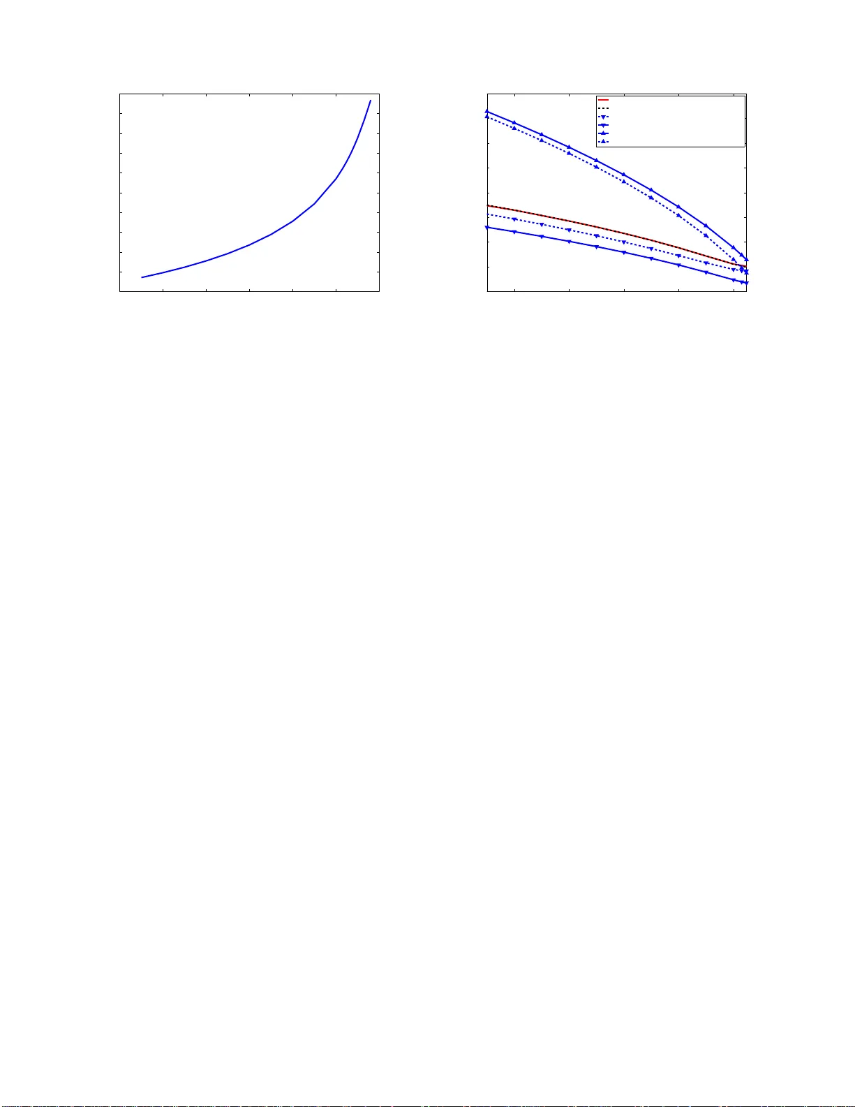
Capacity of The Discrete-T ime Non-Coherent Memoryless Gaussian Channels at L o w SNR Z. Rezki and David Haccoun ´ Ecole Polytechnique de Montr ´ eal, Email: { zouheir .rezki,david.hac coun } @poly mtl.ca Franc ¸ ois Gagnon ´ Ecole de technologie sup ´ eri eure, Email: francois.gagnon@etsmtl.ca Abstract — W e address the capacity of a discre te-time m emoryl ess Gaussian channel, where the channel state informa tion (CSI) is neither a vail able at the transmitter nor at the recei v er . The optimal capacity- achie ving input d istrib ution at low signal -to-noise ratio (SNR) is precisely characte rize d, and the e xact capacity o f a non-coher ent channel is deri ved. The deriv ed rel ations allow to better understanding the capacity of non-coher ent channels at lo w SNR. Then, we c ompute the non- coher ence penalty and give a more prec ise charac teriza tion of the sub- linear term in SNR. F inally , in order to get more insight on how the optimal input var ies with SNR, upper and lower bounds on the non-zero mass point location of the capacity-achie ving input are giv en. I . I N T RO D U C T I O N In wireless communication, the channel estimation at the recei v er is not often possible due, for instance, to the high mobility of t he sender or the receiver or both. T herefore achieving reliable communication ov er fading channels where the channel state i nformation (CSI) is av ail able neither at the tran smitter nor at the recei v er , is of a pa rticular interest. When C SI is not av ail able at both ends, computing the channel capacity , kno wn as the non-coherent capacity , as well as computing the optimal input distri bution achie ving this capacity , for both SISO and MIMO channels, was addressed by Marzetta and Hochwald using a block fading channel [1]. The non-coherent capacity was also computed as a function of t he number of tr ansmit and recei ve antennas as well as the coherence time at high S NR in [2]. At a lo w SNR regime, it was also shown that to a first order of magnitude of t he S NR, there is no capa city penalty for not kno wing the channel at the receiv er which is not t he case at the high SNR regime [2] [3], [4]. Recently , this power ef ficiency at a low SNR regime or equiv alently at a large channel bandwidth has motiv ated work t o wards a better understanding of the non-co herent capacity at a l o w S NR regime [5], [6], [7] for both SISO and MIMO channels using sev eral fading models. For a discrete-time channel, computing t he non-coherent capacity is a rather tedious task [ 8] [9]. The main dif ficulty i n computing the non-cohere nt capacity reli es on the fact that the capacity-achie ving input distribution is discrete with a finite number of mass points, where one of them is located at the origin. The number of these mass points increases with the signal-to-noise ratio (S NR). S ince no bound on the number of mass points with respect to S NR is actually av ail able, it is ve ry dif ficult t o find closed form expressions for both the achiev able capacity and t he optimal input distribution for all S NR v alues. Fortunately , numerical computation of the capacity and the optimal input distri bution has been made possible using t he Khun- T uck er condition w hich is a necessary and suf ficient condition for optimality , for of a SIS O channel [ 8] and for a MIMO channel [9]. In [ 10], the channel mutual information at low SN R is computed and thus t he capacity of a discrete t ime non-coheren t memoryless channel is obtained through numerical optimization. Ho we ver , the frame work presented in [10] does not provide any insight on the capacity behav ior at low SNR. In this paper , we analyze the capacity of a discrete time non- coherent memoryless Rayleigh fading SISO channel at low SNR. The main contributions of this paper are: 1) Deriv ation of an analytical closed form of the channel mutual information at l o w SNR, which may also be considered as a lo wer bound on the channel mutual i nformation for an arbitr ary SNR v alue. 2) Deriv ation of a fundamental relation between the capacity- achie ving input distribution and the SNR value, from which an exa ct capacity expression is deduced at low SNR. 3) Deriv ation of upper and lower bounds on the non-zero mass point location of the optimal input, which a llow to d educe lowe r and upper bound s respectiv ely on the non-co herent capacity at lo w SNR. The paper is organized as follo ws. S ection II presents the system model. In section III, we deriv e a closed form expression of t he channel mutual information at low SNR which is also a l o wer bound on the channel mutual information at all S NR values. The optimal input distri bution as well as the non-co herent capacity are computed in Section IV. Numerical results are rep orted in Section V a nd Section VI concludes the paper . I I . C H A N N E L M O D E L W e consider a discrete-time memoryless Rayleigh-fad ing channel gi ven by: r ( l ) = h ( l ) s ( l ) + w ( l ) , l = 1 , 2 , 3 , ... (1) where l is the discrete-time index , s ( l ) is the channel input, r ( l ) is the channel outp ut, h ( l ) is the fading coefficient and w ( l ) is an additiv e noise. More specifically , h ( l ) and w ( l ) are independ ent comple x circular Gaussian random variables w ith mean zero and variances σ 2 h and σ 2 w , respectiv ely . The input s ( l ) is subject t o an average po wer constraint, that is E [ | s ( l ) | 2 ] ≤ P , where E [ . ] indicates the expec ted value. It is assumed that the channel state information is av ail able neither at the t ransmitter nor at the receiv er . Ho we v er , ev en though the exact v alues of h ( l ) and w ( l ) are not kno wn, their statistics are, at both ends. S ince the channel defined in (1) is stationary and memoryless, the capacity achie ving statistics of the input s ( l ) are also memoryless, independ ent and identically distribu ted (i.i.d). Therefore, for si mplicity we may drop the time inde x l in (1). Consequently , the distribution of the channel output r conditioned on the input s can be obtained after av eraging out the random f ading coef fi cient h , yielding: f r | s ( r | s ) = 1 π ( σ 2 h | s | 2 + σ 2 w ) exp » −| r | 2 σ 2 h | s | 2 + σ 2 w – . (2) Noting that in (2), the conditional output distribution depends only on the squared magnitudes | s | 2 and | r | 2 , we wil l no l onger be concerned with complex quantities but only with their squared magnitudes. Let I LB ( x 1 , a ) = ( a − a h ln (1+ x 2 1 ) x 2 1 + 1 1+ x 2 1 + x 2 1 1+ x 2 1 · 2 F 1 “ 1 , 1 x 2 1 , 1 + 1 x 2 1 , − (1+ x 2 1 )( x 2 1 − a ) a ”i − ln “ 1 − a x 2 1 ” − ln “ 1 + a (1+ x 2 1 )( x 2 1 − a ) ” if x 1 > √ a, 0 if x 1 = √ a (9) x 2 1 − (1 + x 2 1 ) ln(1 + x 2 1 ) − π „ a x 2 1 + x 4 1 « 1 x 2 1 csc „ π x 2 1 « » 1 + x 2 1 − π cot „ π x 2 1 « + ln „ a x 2 1 + x 4 1 «– = 0 . (11) y = | r | 2 /σ 2 w and let x = | s | σ h /σ w . Conditioned on the i nput, y is chi-square distributed with two de grees of freedom: f y | x ( y | x ) = 1 (1 + x 2 ) exp » − y 1 + x 2 – , (3) with the av erage power constraint E [ x 2 ] ≤ a , where a = P σ 2 h /σ 2 w is the SNR per symbol ti me. I I I . T H E C H A N N E L M U T UA L I N F O R M A T I O N For the chann el (3), the mutual information is giv en by [11]: I ( x ; y ) = Z Z f y | x ( y | x ) f x ( x ) ln f y | x ( y | x ) f ( y ; x ) ( y ; x ) dxdy . (4) The capacity of channel (3) is the supremum C = sup E [ x 2 ] ≤ a I ( x ; y ) (5) ov er all input distributions that meet the constraint power . The existence an d uniqueness of su ch an inpu t distribution w as establishe d in [8]. More specifically , the optimal input distribution for channel (3) is discrete with a fi nite number of mass points, where one of t hem is necessarily null. That is, the capacity (5) is expresse d by C = max E [ x 2 ] ≤ a N − 1 X i =0 p i Z ∞ 0 f y | x i ( y | x i ) ln " f y | x i ( y | x i ) P j p j f y | x j ( y | x j ) # dy , (6) where x 0 = 0 < x 1 < x 2 . . . < x N − 1 are t he mass point l ocations and where p 0 , p 1 . . . , p N − 1 their probabilities respectiv ely . Since we focus on the low SNR regime, we may use in (6) a discrete input distribution with two mass points, where one of them is null, to obtain the optimal capacity at lo w SNR [8]. Furthermore, this on-off signaling also provides a lower bound on the non-coherent capacity for all SNR values. That is, a lo wer bound on the capacity may be express ed by: C LB = max E [ x 2 ] ≤ a I LB ( x ; y ) , (7) where I LB ( x ; y ) is a lower bound on the channe l mutual information I ( x ; y ) gi ven by: I LB ( x ; y )= I LB ( x 1 , p 1 ) = 1 X i =0 p i Z ∞ 0 f y | x i ( y | x i ) ln " f y | x i ( y | x i ) P j p j f y | x j ( y | x j ) # dy , and the average constraint po wer becomes: p 1 x 2 1 ≤ a . Note that the optimization problem in (7) deals with only two unkno wns p 1 and x 1 . Furthermore, it is proven belo w that further simplificati ons can be obtained, using the fact that I LB ( x 1 , p 1 ) is monotonically i ncreasing in x 1 and thus the problem at hand may be reduced to a simpler maximization problem without constraint. W e summarize this result in Lemma 1. Lemma 1: The optimal capacity at low SNR and a lower bound on it for all SNR values is gi ven by: C LB = max x 1 ≥ √ a I LB ( x 1 , a ) , (8) where I LB ( x 1 , a ) is t he channel mutual information for a giv en mass point location x 1 and a giv en SNR v alue a , given by (9) at the top of the page, and where 2 F 1 ( · , · , · , · ) is the Gauss hypergeo metric function. Furthermore, the constraint po wer holds with equality and we hav e: E [ x 2 ] = p 1 x 2 1 = a . Pr oof: The proof is presented in [12]. In Lemma 1, t he existence of a maximum for a give n SNR value a is guaranteed by the continuity of I LB ( x 1 , a ) and the fact that i t is bounded with respect to x 1 ov er the interv al [ √ a, ∞ [ . The existence of such a maximum was ri gorously established in [12]. Clearly , the maximization (8) is reduced to solving t he equation ∂ ∂ x 1 I LB ( x 1 , a ) for a given S NR value a . Ideally , an analytical solution would provid e an insight as t o how the non-coh erent capacity and t he on-off signaling vary with the S NR. Howe v er , solving such an equation for arbitrary SNR v alues is very ambitious since it comes to finding an analytical solution to in v olved transc endental equations. Ne verth eless, it i s of interest to focus on the low SNR regime to get the benefit of some advantag eous simplifications in order to el ucidate the non- coherent capacity behav ior at lo w SNR. I V . N O N - C O H E R E N T C A PAC I T Y A T L OW S N R In this section, we will use L emma 1 to derive a fundamental analytical relati on between the optimal input distribution at a low SNR regime and the particular SNR value a . W e sho w in Theorem 1 t hat this fundamental relati on holds up to an order of a strictly less than 2. As is shown below , the deriv ed rel ation i s very useful since it allo ws computing the optimal input distribution for a giv en SNR v alue a while providing a rigorous characterization as to ho w the non zero mass point locations and their probabilities vary with a . Moreo ver , the deri ved relation may be used to compu te the exact non-cohere nt capacity at lo w SNR values. A. A fundamental relation between the optimal input and the SNR W e present the fundamental relati on between the optimal input distribution and the SNR v alue in the following theorem. Theor em 1: At a l o w S NR value a , the optimal input probability distribution for an order of magnitude of a strictly less t han 2 ( o ( a 2 − ǫ ) for an arbitrary positiv e ǫ ), is giv en by: f x ( x ) = ( x 1 with probability p 1 = a x 2 1 , 0 with probability p 0 = 1 − p 1 , (10) where x 1 is the solution of the equation (11) giv en at the top of the page. Furthermore, the non-coheren t channel capacity is giv en by: C ( a, x 1 ) = a − a · ln (1 + x 2 1 ) x 2 1 − a 1+ 1 x 2 1 · π csc “ π x 2 1 ” “ 1 x 2 1 + x 4 1 ” 1 x 2 1 1 + x 2 1 (12) Pr oof: The proof is presented in [12]. Clearly , ( 11) is also a transcendental equation, for which determining an analytical solution is a very tedious task. Although it is very in v olved to deri ve an analytical solution of (11) in the form of x 1 = f ( a ) , it i s of interest from an engineering point of view , to a = exp » x 2 1 W ` k, ϕ ( x 1 ) ´ − x 2 1 + π cot ` π x 2 1 ´ + ln ( x 2 1 ) + ln (1 + x 2 1 ) − 1 – , (14) ϕ ( x ) = − sin ( π x 2 )( − x 2 + ln (1 + x 2 ) + x 2 ln (1 + x 2 )) π x 2 · exp − π cot ` π x 2 ´ x 2 + 1 + 1 x 2 ! . (15) resolve (11) numerically and obtain the optimal x 1 for a gi v en SNR v alue a . One m ay then get the v alue o f the non-cohe rent capacity from (12). Moreo v er , (11) provides some insight on the behavio r of x 1 as a tends tow ard zero. For example, using ( 11), one may determine the limit of x 1 as a tends toward zero. T o see t his, let M be t his l imit and let us assume that M is finite. From [6], [8], we kno w that for the optimal input distribution, t he non-zero mass point location x 1 is greater t han one. T hus, its limit as a tends to ward zero is greater or equal than one: M ≥ 1 . T hen, taking the limits on both si des of (11) as a goes to zero yields: M 2 − (1 + M 2 ) ln (1 + M 2 ) = 0 . (13) That is, if M is fi nite, it wou ld be equal to zero, t he unique solution to ( 13), but this i s impossible since M ≥ 1 . H ence, consistently with [6], [8], lim a → 0 x 1 = ∞ . Furthermore, we ha ve found that (11) may be written more con veniently as (14) at the t op of the page, with k = − 1 if a ≤ a 0 and k = 0 elsewhere, and where W ( · , · ) is t he Lambert function, with ϕ ( x ) give n by (15) at the top of the page too. Also, a 0 is the solution of (11) for x 1 = x 0 , where x 0 is the root of t he equation ϕ ( x ) = − 1 e . The number − 1 e comes out in our analysis from the fact that it is the unique point shared by the principal branch of the Lambert function W (0 , x ) and the branch w ith k = − 1 , W ( − 1 , x ) . That is W (0 , − 1 e ) = W ( − 1 , − 1 e ) . This guarantees the continuity of a in (14) for all x 1 v alues. Numerically , we hav e found t hat a 0 = 0 . 0582 and x 0 = √ 3 . 93388 . Hence, (14) may also be vie wed as a fundamental relation between the optimal i nput distribution and the SNR a for discrete-time non-coherent memoryless Rayleigh fading channels at low SNR. On the other hand, (14) provides the global answer as to ho w the non-zero mass point location of the optimal on-off signaling and the SNR are linked t ogether . For this purpose, a simple analysis of (14) has been done and some important results are recapitulated in the following corollary . Cor ollary 1: According to ( 14), we hav e: 1) For al l a ≤ a 0 , a 0 = 0 . 0582 , a is an decreasing function with respect to x 1 and for all a > a 0 , a is an i ncreasing function of x 1 . 2) For all a , x 1 ≥ x 0 , where x 0 = √ 3 . 93388 . 3) lim x 1 →∞ a = 0 . Corollary 1 agrees wi th [8] where it was sho wn using computer simulation that the non-zero mass point l ocation passes through a minimum before moving upward. Howe v er , by specifying the edge point ( x 0 , a 0 ) , Corollary 1 gives a more precise characterization con- cerning t his peculiar behavior of the non-zero mass point l ocations. Furthermore, C orollary 1 also refines the lower bound on x 1 , x 1 > 1 and deriv es x 0 as an i mprov ed l o wer bound on the non-zero mass point location at low SNR. Moreo ve r , from (14), we may write: ln ( a ) + x 2 1 = x 2 1 W ` k, ϕ ( x 1 ) ´ + π cot ` π x 2 1 ´ + ln ( x 2 1 (1 + x 2 1 )) − 1 . (16) It is then easy to check that the right hand side (RHS) of (16) is a decreasing function of x 1 for x 1 < x 0 , which yields an upper bou nd on x 1 : x 2 1 ≤ − ln ( a ) + ξ 0 , (17) where ξ 0 = ln ( a 0 ) + x 2 0 , which is again consistent with the upper bound deri ve d in [6]. Note that the upper bound (17) is valid for all a ≤ a 0 whereas the upper bound provided in [6] holds for a ≪ a 0 for which ξ 0 is negligible. On the other hand, combining (17) and the lo wer bound on x 1 provid ed in Corollary 1 one may obtain: a α x 2 0 ≤ a α x 2 1 ≤ a α ( ξ 0 − ln ( a )) . (18) for all α > 0 . That is: lim a → 0 ` a α x 2 1 ´ = 0 , (19) which means that a α tends tow ard zero faster than x 2 1 does tow ard infinity . This result may also be used to gain further insight on the capacity behavior at lo w S NR. For instance, from (12), we may wr ite the non-cohe rent capacity as: C ( a ) = a + o ( a ) , (20) where o ( a ) = − a · ln (1+ x 2 1 ) x 2 1 − a 1+ 1 x 2 1 · π csc „ π x 2 1 «„ 1 x 2 1 + x 4 1 « 1 x 2 1 1+ x 2 1 , meaning that the non-co herent capacity v aries li nearly wit h a at lo w SNR and hence non-coherent communication at lo w S NR may be qualified as energy ef ficient communication. B. Ener gy efficiency and non-coher ence penalty In general, the capacity of a channel i ncluding a Gaussian channel and a Rayleigh channel varies linearly at low SNR [6]. T he diffe rence between these channels in terms of capacity can only be explained by the sub-linear term o ( a ) in (20). The sub-linear term has been defined in [6] as: ∆( a ) := a − C ( a ) . (21) At lo w SNR, the sub-linear term ∆( a ) i s also related to the energ y- efficien cy . L et E n be the tr ansmitted energy in Joules per information nat, then we hav e: E n σ 2 w · C ( a ) = a. (22) Using (21), we can write: E n σ 2 w = 1 1 − ∆( a ) a ≈ 1 + ∆( a ) a , (23) where the approximation holds if ∆( a ) a is sufficiently small. Note t hat if ∆( a ) a → 0 , t hen from (21) and (23), we have respectiv ely: C ( a ) ≈ a and E n σ 2 w ≈ 1 , which implies that the highest ener gy efficienc y of - 1.59 (dB) per information bit could be t heoretically achie v ed. For a Gaussian channe l and a fading channel under the coherent assumption, the sub-linear terms are respectiv ely giv en by [6]: ∆ AW GN ( a ) = 1 2 a 2 + o ( a 2 ) (24) ∆ coher ent ( a ) = 1 2 E [ k h k 4 ] a 2 + o ( a 2 ) (25) For a non-coh erent Rayleigh fad ing channel, the sub-linear term can be computed using (12): ∆( a ) = a · ln (1 + x 2 1 ) x 2 1 + a 1+ 1 x 2 1 · π csc “ π x 2 1 ” “ 1 x 2 1 + x 4 1 ” 1 x 2 1 1 + x 2 1 . ( 26) 10 −10 10 −8 10 −6 10 −4 10 −2 1.8 2 2.2 2.4 2.6 2.8 3 3.2 SNR Non−zero mass point location Non−zero mass point location (simulation) Non−zero mass point location given by (16) Figure 1. Locati on of non-zero mass point versus the SNR val ue a (linea r). Note that at very low SNR and following (26), ∆( a ) a con verges to zero making the non-coherent Rayleigh channel also energy efficient. Ho we ver , as SNR increases, the con vergence of ∆( a ) a to zero is slo wer than ∆ AW GN ( a ) a and ∆ coherent ( a ) a . This could be seen from (19) indicating that x 1 con verges slo wer to infinity than a does to zero. In the range of SNR valu es of interest, we may define the non- coherence penalty per SNR as: C coher ent ( a ) − C ( a ) a . (27) where C coher ent is the channel capacity under coherent assump tion. No w , from [6], we can write C coher ent as: C coher ent ( a ) = a + O ( a ) = a + o ( a 2 − α ) , (28) for any 1 > α > 0 . Recalling that the non-coherent capacity in (12) was obtained using series decomposition to an order strictly smaller than 2 ( o ( a 2 − ǫ ) for an arbitrary positive ǫ ), t hen combining (12) and (28), we deriv e the exact non-cohe rence penalty per SNR up t o this order: C coher ent ( a ) − C ( a ) a = C coher ent − C C coher ent = ln (1 + x 2 1 ) x 2 1 + a 1 x 2 1 π csc “ π x 2 1 ” “ 1 x 2 1 + x 4 1 ” 1 x 2 1 1 + x 2 1 (29) Note that the non-coherence penalty is equal to the sub-linear term ∆( a ) . Now using ( 19), div iding both sides of (29) by a α , ( α > 0 ) and taking the limit as a tends to zero yields: C coher ent ( a ) − C ( a ) ≫ a 1+ α , ( 30) where ≫ means: lim a → 0 C coherent ( a ) − C ( a ) a 1+ α = ∞ . Inequality (30) indicates that not only non-coherence penalty is much greater than a 2 as was established in [5], but more precisely , it is much greater than a 1+ α since a 1+ α ≫ a 2 , 1 > α > 0 . Again, this result is i n full agreement with [6]. In this subsection, we have discussed exact closed forms of the optimal i nput distribution and the non-coherent capacity based on the f undamental relation (11) or equiv alently (14). Howe v er , one may be interested in deriving simpler lower and upper bounds on these quantities in order to provide more insight on ho w they vary wi th the SNR v alue a . This is discussed nex t. 10 −10 10 −8 10 −6 10 −4 10 −2 10 −12 10 −10 10 −8 10 −6 10 −4 10 −2 SNR Capacity in natts Linear approximation Simulation and (12) Figure 2. Non-cohere nt capa city ve rsus the SNR v alue a (linear). C. Upper and lower bound s on the non-coher ent capacity Considering (14), since we are interested in the lo w SNR re gime, we assume for simplicity that a ≤ a 0 . T hus the Lambert function in (14) is the branch with k = − 1 , W ( − 1 , x ) . A lo wer bound on the non-cohere nt capacity is easily obtained by combining (17) and ( 12) and will be referred to as C LB ( a ) . W e no w derive the lo wer bound on the optimal non -zero mass point location and the upper bound on the non-cohe rent capacity in Theorem 2. Theor em 2: At low SNR values a , a lower bound on the optimal non-zero mass point location is give n by: x 1 ,LB = y v u u t − W − 1 , ϕ “ y − ln ` − ϕ ( y ) ´ ” ! , (31) where y = q 1 + ln 1 a . F urthermore, an upper bound on the non- coherent capacity can be obtained from (12) as: C U B ( a ) = C ( a, x 1 ,LB ) (32) Pr oof: The proof is presented in [12]. V . N U M E R I C A L R E S U LT S A N D D I S C U S S I O N The curves in Fig. 1 show respectiv ely , the non-zero mass point location of the capacity-achiev ing i nput distri bution x 1 obtained using maximization (8), and the one obtained using relation (11) or equiv alently ( 14). As can be seen from F ig. 1, the t wo curves are undistinguishable at low S NR, confirming that (15) is exact at lo w SNR. As the SNR i ncreases, a small discrepanc y between the two curv es starts to appear . This is expected since (14) holds for up to an order of magnitude strictly smaller than 2 and thus for small SNR v alues, (but not smaller than about 2 . 10 − 2 ), a discrepancy may appear . Nevertheless, ev en for an SNR greater than 2 . 10 − 2 , the curve obtained using (14) is very instructiv e especially as it follo ws the same shape as the one obtained by simulation results. An interesting future work would be to use (15) in order t o understand why a ne w mass point should appear as the SN R increases. I t should be mentioned that the discrepancy observ ed in Fi g. 1 may be rendered as small as desired using high order series expansion. Howe ver , the analysis would be unre warding ly too complex . Figure 2 depicts the non-coherent capacity curves. Again, the curve obtained by computer simulation and the one obtained using (12) 10 −12 10 −10 10 −8 10 −6 10 −4 10 −2 10 0 0.25 0.3 0.35 0.4 0.45 0.5 0.55 0.6 0.65 0.7 0.75 SNR Non−coherence penalty Figure 3. Non-cohere nce pena lty per SNR versus the SNR valu e a (linea r). are undistinguishable. More interestingly , the discrepancy observed at not very low S NR values in Fig. 1 has vanished, implying that the capacity is not very sensitiv e to the non-zero mass point location. Also shown in Fig. 2 is the linear approximation C ( a ) = a , which is an upper bound on t he capacity . As can be noticed in F ig. 2, the linear approximation follows t he same shape as the exact non- coherent capacity curves at l o w SNR and becomes quite loose for SNR v alues greater t han 10 − 2 . This implies that the sub-linear term defined in (21) is much more important at these SNR values. This can be seen in Fig. 3 where we hav e plotted the non-coheren ce penalty percentage giv en by (29). Figure 3 confirms that t here is no substantial gain in the channel kno wledge in a capacity sense at very lo w SNR, thus indicating that non-cohe rent communication is almost as power -ef ficient as A W GN and coherent communications. As the SNR increases, a non-coherence penalty begins t o appear reaching up to 70% . The derived upper and lo wer bound s on the non zero mass point locations gi ven respectiv ely by ( 17) and ( 31) as well as the bounds deri ved in [6] are plotted i n F ig. 4 along with the exact curves at lo w SNR. As can be seen in Fig. 4, the upper bou nd in [6], albeit tighter than (17), crosses the ex act curv es at about 2 . 10 − 2 . At these not so low S NR values, t he derive d bound in [6] is no longer an upper bound, consistently with our discussion in subsection IV -A. On the other hand, the lower bound (31) is ti ghter than the one deriv ed in [6] for all SNR values. V I . C O N C L U S I O N In this paper, we have addressed the analysis of the capacity of discrete-time non-coherent memoryless Gaussian channels at low SNR. W e hav e computed explicitly the channel mutual information at low SNR which is also a lower bound on the channel mutual information, albeit not necessarily at lo w S NR values. Using the deri ved expression of the channe l mutual information, we hav e been able to provide a f undamental relation between the non-zero mass point location of the capacity-achie ving input distribution and the SNR. This fundamental relation brings the complete answer about ho w t he optimal input distribution varies with the power constraint at low SNR. It also provides an analytical explanation on what was pre viously observed through computer simulation in [8] about the peculiar behavior of the non-zero mass point location at low SNR v alues. The exact non -coherent capacity has been deriv ed and insights 10 −10 10 −8 10 −6 10 −4 10 −2 1.5 2 2.5 3 3.5 4 4.5 5 5.5 SNR Non−zero mass point location Non−zero mass point location (simulation) Non−zero mass point location given by (14) The lower bound given by (31) The lower bound in [6] The upper bound given by (17) The upper bound in [6] Figure 4. Exact non-zero mass point locat ions and the deri v ed upper and lo wer bounds as well as those reported in [6] versus the SNR va lue a (linea r). on the capacity behavior which can be gained through functional analysis has been shown . In order to better understand ho w the non-zero mass point location v aries with the SNR, we have also deriv ed lower and upper bounds which hav e been compared to recently deriv ed bounds. The ne wly deri ved lower bound i s tighter for all SNR values of interest, whereas some what looser , the upper bound was shown to hold for larger SNR v alues. R E F E R E N C E S [1] T . L. Marzet ta and B. M. Hochwald, “Capac ity of a Mobile Multiple- Antenna communication Link in Rayleigh Flat Fadi ng , ” IEEE T rans. on Informatio n Theory , vol. 45, no. 1, pp. 139-157, Jan. 1999. [2] L izhong Zheng and David N. C. Tse “Communic ation on the Grassmann Manifold : A Geometric Approach to The Noncoherent Multipl e-Antenn a Channel , ” IEEE T rans. on Inf ormation Theory , vol. 48 , no. 2, pp. 359-38 3, Feb . 2002. [3] R. S. Kennedy , F ading Dispersive Communicat ion Channels , New Y ork: W ile y , 1969. [4] I. E. T elat ar and D. Tse “Capacit y and Mutual Information of Wideb and Multipl ath Fading Chan nels, ” IE EE T rans. on Information Theory , vol . 46, no. 4, pp. 1384-1400, July 2000. [5] Sergio V erd ´ u, “Spectral Ef ficien cy in the Wi deband Regi me, ” IEEE T rans. on Information Theory , v ol. 48, no. 6, pp. 1319-1343, June 2002. [6] L izhong Zheng, Davi d N. C. Tse and Murie l M ´ edard “Channe l Cohere nce in The L o w-SNR Regime, ” IEEE T rans. on Information Theory , vol. 53, no. 3, pp. 976-997, Marc h 2007. [7] Siddharth Ray , Muriel M ´ eda rd and Lizhong Z heng “On Noncoherent MIMO Channels in The W ideba nd Regime: Capacity and Reliabilit y , ” IEEE T rans. on Info rmation Theory , vol. 53, no. 6, pp. 1983-2009, June 2007. [8] Ibrahim C. Abou-Fayc al, Mitchell D. Trott and Shlomo Shamai(Shitz), “The Capacity of Discrete-T ime Memoryle ss Rayleigh -Fadi ng Channels, ” IEEE T rans. on Info rmation Theory , vol. 47, no. 4, pp. 1290-1301, May 2001. [9] R. R. Perera, K. Nguyen, T .S. Pollock; and T .D. A bhayapa la, “Cap acity of Non-Cohere nt Rayleigh Fading MIMO Channels. ” Communication s, IEE Pr oceedi ngs- , V o l.153, Iss.6, Dec. 2006 Pages: 976-983 [10] S. de la Kethu lle de Ryhov e, N. Marina, and G. E. Ø ien, “On The Capacit y and Mutual Information of Memoryless Noncohere nt Rayle igh-Fa ding Chann els, ” 2006. [Onli ne]. A va ilable : http:/ /www .citebase.or g/abstra ct?id=oai:arXiv .org:cs/0605075 [11] R. G. Gallager , Information Theory and Reliable Communication , New Y ork: W ile y , 1968. [12] Z ouheir Rezki, David Hacco un, and Franc ¸ ois Gagnon “Capacity of The Discrete -Ti me Non-Cohere nt Memoryless Rayleig h Fadi ng Chan nels at L ow SNR, ” 2008. [Online]. A v ailab le: http:/ /www .citebase.or g/abstra ct?id=oai:arXiv .org:0801.0581