Maximum likelihood estimation of a multidimensional log-concave density

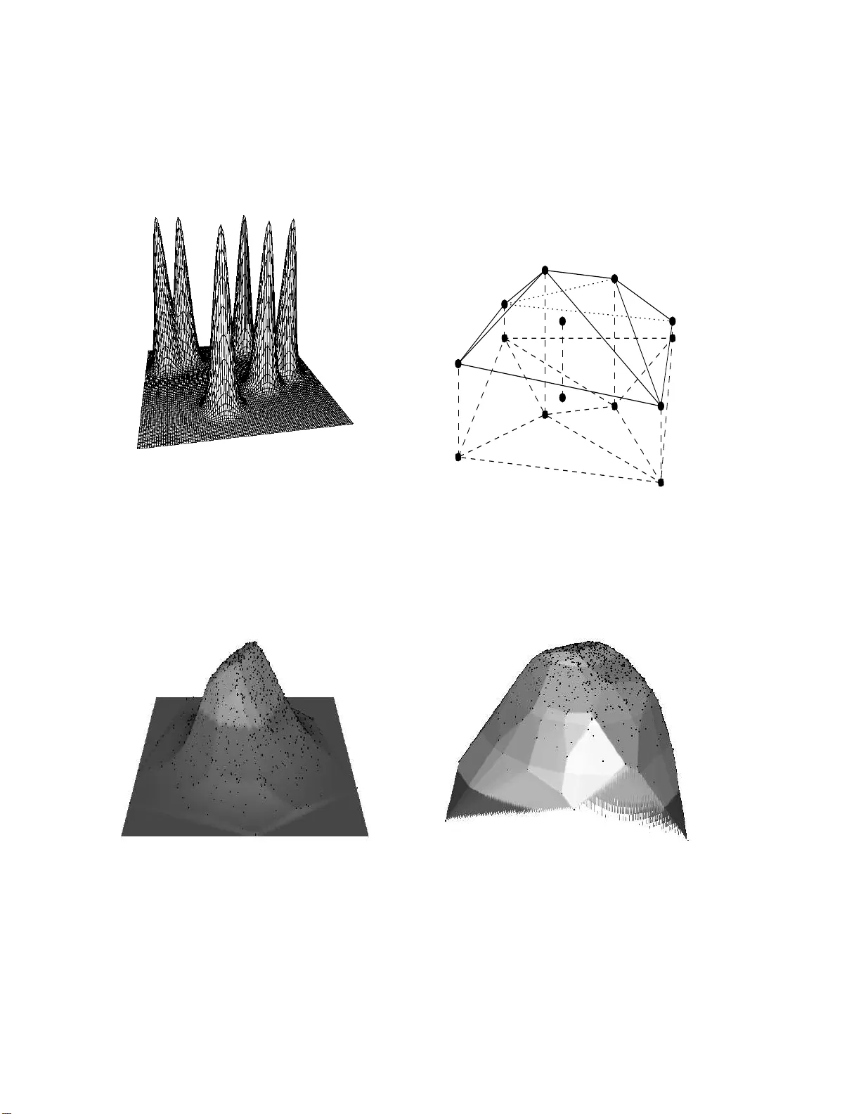
Maxim um lik eliho o d estimation of a m ultidimensional log-conca v e d ensit y Madeleine Cule & Ric hard Samw orth ∗ Statistical Lab oratory Univ ersity of Cambridge Mic hael Stewart Sc ho ol of Mathematics and Statistics Univ ersity of Sydney Octob er 22, 2018 Abstract Let X 1 , . . . , X n b e i ndep endent and identicall y d istribu t ed random vectors with a log-concav e (Leb esg ue) density f . W e ﬁrst prov e that, with probability one, there exists a unique maxim um lik elihoo d estimator ˆ f n of f . The use of this es timator is attractiv e because, u nlik e kernel density estimation, the metho d is fully aut o matic, with no smooth ing parameters to choose. Although the existence p roof is non-constructive, we are able to reform ulate the issue of computing ˆ f n in terms of a n on-diﬀeren tiable conv ex optimisati on problem, and thus com bine tec hniques of computational geometry with Shor’s r -algori thm to pro duce a sequence that conv erges to ˆ f n . F or the mo derate or large sample sizes in our simulatio ns, the maximum likelihoo d estimator is sho wn to pro vide an impro v ement in p erforma nce compared with k ernel-based metho ds, ev en when w e allo w th e u s e of a th eo retical, op t i mal ﬁxed b a ndwidth for th e kernel estimator t h at w ould not b e a v ailable in practice. W e also present a real data clustering ex a mple, which sho ws that our metho dology can b e used in conjunction with the Ex p ectation–Maximisatio n (EM) algorithm to ﬁt ﬁnite mix t ures of log-conca ve den sities. An R versio n of the algorithm is av ailable in the pac k age LogConcDEAD – Log-Conca ve D ensi ty Estimation in A rbitrary D ime nsions. Keywords: Computational g eometry , log-concavit y , maxim um lik eliho od estimation, non- diﬀerentiable conv ex optimisation, nonparametric density estimation, Shor’s r -algor ithm 1 In tro duction Mo dern nonparametr ic density estimation beg a n with the in tro duction of a kernel density estimator in the pioneering work of Fix and Ho dges (195 1), later republished as Fix and Hodg es (1989). F or ∗ A ddr e ss for c orr esp ondenc e : Richa rd Samw orth, Statistical Lab oratory , Cen tre for Mathematical Sciences, Wilb e rforce Road, Cam bridge, UK . CB3 0WB. E-mail: r.j.samwo rth@statslab.cam.ac.uk. 1 independent and iden tically distributed rea l-v alued observ ations, the app ealing a symptotic theory of the mean integrated squar ed error was provided by Rosenblatt (1956) and Parzen (196 2). This theo ry leads to an asymptotically optimal choice o f the smo othing parameter , or bandwidth. Unfortunately , how ever, it depends on the unknown density f through the integral o f the square of the second deriv ative of f . Consider able eﬀort has ther e f ore b een fo cused o n ﬁnding metho ds o f automatic bandwidth s election (cf. W and and Jones, 19 95, Chapter 3 , and the reference s therein). Although this has resulted in alg orithms, e.g. Chiu (19 9 2), tha t achieve the optimal r ate of co n vergence of the relative er ror, namely O p ( n − 1 / 2 ), wher e n is the sample size, goo d ﬁnite sa mple p erformance is b y no mea ns guaranteed. This problem is co mpounded when the observ atio ns take v alues in R d , w he r e the g eneral kernel estimator (Deheuvels, 1977) requires the sp eciﬁcation of a symmetric, pos itive deﬁnite d × d band- width matrix. The diﬃculties inv olved in making the d ( d + 1) / 2 choices for its en tries mean that attent ion is often res tricted either to bandwidth matr ices that are diago nal, or even to those that a re scalar multiples of the identit y matrix. Of course, pr actical issues of automatic bandwidth selection remain. In this pap er, w e pr opose a fully automatic no nparametric estimator o f f , w ith no tuning parameters to be chosen, under the condition that f is log-co nca ve – that is , log f is a concav e function. The class of log -concav e densities has many a ttr a ctiv e prop erties and has b een w ell-studied, particularly in the economics, sampling and reliabilit y theory literature. See Section 2 for fur ther discussion o f examples, applications and prop erties of log-concave densities. In Section 3, we show that if X 1 , . . . , X n are indep enden t and identically distributed ra ndom vectors with a log-concav e density , then with pro babilit y one there exists a unique log-concav e density ˆ f n that maximises the likelihoo d function, L ( f ) = n Y i =1 f ( X i ) . Before contin uing, it is worth noting that without any shape co nstrain ts on the densities under consideratio n, the likelihoo d function is un b ounded. T o see this, we could deﬁne a s e q uence ( f n ) of densities that repr esen t successively close appr o x imations to a mix tur e o f n ‘spikes’ (o ne on each X i ), such as f n ( x ) = n − 1 P n i =1 φ d,n − 1 I ( x − X i ), where φ d, Σ denotes the N d (0 , Σ) density . This sequence satisﬁes L ( f n ) → ∞ as n → ∞ (cf. Fig ure 1). In fact, a mo diﬁcation of this argument may b e used to show that the likeliho od function remains unbounded even if w e restrict attention to unimodal densities. Figure 2 gives a diagram illustra ting the structure o f the maximum lik eliho od es tim ator o n the logarithmic sca le. This structure is most easily visua lised for t w o-dimensiona l data, where one can imagine asso ciating a ‘tent pole’ with ea ch o bserv ation, extending vertically out of the plane. F or certain tent p ole heights, the graph of the logarithm of the maximum lik eliho od estimator can b e thought of as the r oof of a taut tent stretched over the ten t poles. The fact that the logarithm o f the maximum likelihoo d estimator is o f this ‘tent function’ form constitutes par t of the pr oof of its existence and uniqueness. In Section 4, we discuss the computational problem of how to adjust the n tent p ole heig h ts s o that 2 Figure 1: Without any shap e co ns t raint on the class of densities, the likelihoo d function is un b ounded, beca use w e can ta k e successively close a ppr o ximations to a mix t ure of n ‘spikes’ (one o n each X i ). Figure 2: The ‘tent-lik e’ structure of the gra ph of the logarithm o f the max imum likelihoo d es- timator for biv ariate data. (a) Density (b) Log-density Figure 3: Log-co nca v e maximum likelihoo d es tim ates ba sed on 1000 observ a tions (plotted a s dots) from a sta nda rd biv aria te normal distr ibutio n. 3 the cor responding tent functions co n verge to the logar ithm o f the maximum likelihoo d estimator. One rea s on that this co m putational pr o blem is so c hallenging in more than one dimension is the fact that it is diﬃcult to describ e the set of tent p ole heights that corr espond to concave functions. The key obse rv ation, discussed in Section 4, is that it is pos sible to minimise a mo diﬁed ob jective function that it is conv ex (though non- diﬀer en tiable). This allows us to apply the powerful non-diﬀerentiable conv ex optimisation methodolo gy o f the subgr adien t metho d (Shor , 1 985) and a v a rian t called Shor ’s r -a lgorithm, which has b een implemented by K appel and Kuntsevic h (2000). As an illustra tion of the es tim ates obtained, Figure 3 presents plots of the maximum likeliho od e s ti- mator, and its logar ithm, for 100 0 observ ations from a standa rd biv a riate no rmal distribution. These plots were created using the LogConc DEAD pack age (Cule et al. , 200 8a) in R (R Developmen t Co re T eam, 2008 ) , which exploits the interactiv e surface- plotting so ft ware av ailable in the rgl pack age (Adler and Mur doch, 2007 ). In Sec t ion 5 w e present sim ulations to compar e the ﬁnite-sample perfo rmance of the maximum likelihoo d estimator w ith kernel-based metho ds. The results are strik ing: even when we use the theoretical, optimal bandwidth for the kernel estimato r (o r an a symptotic a ppro ximation to this when it is not av ailable), we ﬁnd that the maxim um likelihoo d estimator ha s a rather smaller mean integrated squared err o r for mo derate or larg e sample sizes, despite the fact that this optimal bandwidth dep ends on prop erties of the density that w ould be unkno wn in pra c t ice. This suggests that the maximum lik eliho o d estimator is able to adapt to the lo cal smoothness of the under lying density automatically . Nonparametric density estimation is a fundament al to ol for the visualisa tio n of str uctu re in ex- plorator y da ta analysis, and has an enormous literature that includes the mo nographs of Devr o ye and Gy¨ orﬁ (1 985), Silverman (1986 ), Scott (19 9 2) and W and and Jones (1995). Our pro posed metho d may certainly b e used fo r this purp ose; ho wev e r, it may also b e used as a n in termediary stage in mor e inv o lved statistical pr ocedures. F o r instance: 1. In classiﬁca tion problems, we hav e p ≥ 2 popula tio ns of interest, and assume in this discussion that these have densities f 1 , . . . , f p on R d . W e observe training data of the form { ( X i , Y i ) : i = 1 , . . . , n } , where if Y i = j , then X i has density f j . The aim is to class if y a new obser v ation z ∈ R d as coming from one of the p opulations. Pr o blems of this t yp e o ccur in a huge v ariety of applica tions, including medical diagnos is, archaeology , ecolo gy etc. – s ee Gordon (1981), Hand (1981 ) or Dev r o y e et al. (1996) for further details and exa mp les. A natural a pproac h to classiﬁcation pro blems is to constr uct densit y estimates ˆ f 1 , . . . , ˆ f p , where ˆ f j is ba s ed on the n j observ a tions, say , from the j th p opulation, namely { X i : Y i = j } . W e may then assign z to the j th p opulation if n j ˆ f j ( z ) = max { n 1 ˆ f 1 ( z ) , . . . , n p ˆ f p ( z ) } . In this co n text, the use of kernel-based estimato rs in general requires the choice o f p separa te d × d ba ndwidt h ma trices, while the co r responding pr o cedure ba sed on the lo g-concav e maximum likelihoo d estimates is again fully a ut omatic. 2. Clustering pr oblems ar e closely rela ted to the classiﬁcatio n problems des cribed above. The diﬀerence is that, in the ab o ve no ta tion, w e do no t observe Y 1 , . . . , Y n , a nd hav e to assig n each of X 1 , . . . , X n to one of the p p opulations. A common tec hnique is based o n ﬁtting a mixture density of the form f ( x ) = P p j =1 π j f j ( x ), where the mixture prop ortions π 1 , . . . , π p 4 are p o sitiv e a nd sum to o ne. Under the ass ump tion that each o f the comp onen t densities f 1 , . . . , f p is lo g-concav e, we sho w in Section 6 that o ur methodolo g y ca n b e extended to ﬁt such a ﬁnite mixture densit y , which need no t itself b e log- c o nca v e – cf. Section 2. W e also illustrate this clustering algor ithm on a Wisconsin brea st c ancer da ta set in Section 6 , where the aim is to separ ate observ atio ns int o benig n and maligna n t co mponent p opulations. 3. A functional of the true underlying density may b e estimated by the c o rrespo nding functional of a density estimato r, s uch as the lo g-concav e maxim um likelihoo d es tima t or. Examples of func- tionals o f in terest include probabilities, such as R k x k≥ 1 f ( x ) dx , momen ts, e.g. R k x k 2 f ( x ) dx , and the diﬀerential entropy , − R f ( x ) log f ( x ) dx . It may b e p ossible to compute the plug-in es- timator base d on the log- c onca v e ma x im um likelihoo d estimator a nalytically , but in Section 7, we sho w that even if this is not p ossible, in many cases o f in terest we can sample from the log-concave maximum likeliho od es tim ator ˆ f n , and hence obtain a Monte Ca r lo estimate of the functional. This nice feature also means that the log- conca ve maximum likeliho od estima- tor can b e used in a Monte Carlo b oots tr ap pro cedure for as sessing uncertaint y in functional estimates – se e Section 7 for further details. 4. The ﬁtting o f a nonparametr ic density estimate ma y give an indica tion o f the v alidity o f a particular s maller mo del (often parametric). Th us, a co n tour plot of the lo g-concav e maximum likelihoo d estimator may provide evidence that the underlying density has elliptical contours, and thus suggest that a mo del tha t ex ploits this elliptical symmetry . 5. In the univ ariate ca se, W alther (2002) describ es metho dology base d on lo g-concav e density estimation for addre s sing the problem of detecting the pr esence of mixing in a distribution. As an application, he cites the Pic kering/Platt debate (Swales, 1 985) on the issue o f whether high blo od pressur e is a disease (in which case observed blo o d press ure measurements should follow a mixture distribution), or s imp ly a lab el attached to peo ple in the rig h t tail of the blo od pressur e distr ibut ion. As a result of our algo rithm for computing the multidimensional log-concave maximum likelihoo d estimator, this metho dology extends immedia t ely to more than o ne dimension. There has b een consider able recent int erest in shap e-restricted no nparametric density es t imation, but most of it has b een co nﬁned to the case of univ a r iate densities, where the computational algorithms are mo r e s t raightforward. Nevertheless, a s was discussed ab o ve, it is in m ultiv ariate situations that the automatic na tur e of the max im um likelihoo d estimator is pa r ticularly v aluable. W alther (200 2), D¨ um bgen and Ruﬁba ch (2007 ) and Pal et al. (2007 ) hav e proved the existence and uniqueness of the log-concave maximum likelihoo d estimator in one dimension and D ¨ um bgen and Ruﬁbach (2007 ), Pal et al. (200 7 ) and Ba la bdaoui et al. (200 8) have s tu died its theo retical pr operties. Ruﬁbach (2007 ) has compared diﬀerent alg o rithms for computing the univ aria te estimato r, including the iter ativ e co nvex minorant algorithm (Gro enebo om and W ellner , 1992; Jong bloed, 19 9 8), and three others. D¨ um bgen et al. (200 7 ) a lso present an Active Set alg orithm, which has simila rities with the vertex direction and vertex reduction algor ith ms described in Gro enebo om et al. (2008). F o r univ ar iate data, it is also well-kno wn that there exist maximum likelihoo d estimators of a non-incr easing density supp o rted on [0 , ∞ ) (Gr enander, 195 6) a nd of a co n vex, decrea s ing dens it y (Gro enebo om et al. , 200 1). In Section 8, w e g iv e a brief concluding discussion, and sugg e st some directions for future r esearch . 5 Finally , we pres en t in App endix A a glo s sary of terms and r esults fro m convex ana lysis and co m- putational geometry that appea r in ita lic s at their ﬁrst occur rence in the main bo dy of the pap er; the references ar e Ro c k afellar (1997 ) a nd Lee (1997). Pro ofs are deferr ed to App endix B, exc ept that the beg inn ing of the proo f of Theorem 2 is giv en in the main text, as the ideas and notation int ro duced are needed in the remainder of the pap er. 2 Log-conca v e densities: e xamples, applications and prop er- ties Many of the most co mm only-encountered parametric families of univ aria te distributions have lo g- c onc ave densities, including the family of normal distributions , ga mma distributions with shape parameter at lea s t one, B e t a( α, β ) distr ibut ions with α, β ≥ 1 , W eibull distributions with shap e parameter at least one, Gum b el, logistic and Laplace densities; see Bagno li and Bergstr o m (1 9 89) for other examples. Univ ariate log-co nca v e densities ar e unimoda l and ha ve fairly light tails – it may help to think of the exp onen tial distribution (where the lo garithm of the density is a linear function on the p ositive half-axis) as a b orderline case. Th us Cauch y , Pareto and lo gnormal densities, for instance, are not log- conca ve. Mixture s of log -conca ve densities may b e log-concave, but in gener al they are not; for insta nc e , for p ∈ (0 , 1 ), the lo cation mixtur e of standar d univ aria te normal densities f ( x ) = pφ ( x ) + (1 − p ) φ ( x − µ ) is log-concave if and only if k µ k ≤ 2. The ass umption of log -conca vity is a p opular one in economics; Caplin and Naelbuﬀ (1991 b) show that in the theory o f elections and under a log- c o nca vit y assumption, the prop osal mo st preferr ed by the mean voter is un bea ta ble under a 64% ma jority r ule. As ano t her e x ample, in the theory of imper fect comp etition, Caplin and Naelbuﬀ (1991a) use log-co nca v it y of the densit y of consumers’ utilit y parameter s as a suﬃcient condition in their pr oof of the ex istence of a pure-stra t egy pr ice equilibrium for a ny num ber of ﬁrms pro ducing any set of pro ducts. See Bagno li and Bergstro m (1989) for many other applicatio ns of log- conca vity to economics . Bro oks (1998 ) a nd Mengersen and Tweedie (19 9 6) have explo it ed the prop erties of log-concave densities in studying the c o n vergence of Marko v chain Monte Carlo sampling pro cedures. An (199 8) lists many useful prop erties of log-co nc ave densities . F o r instance, if f and g are (p ossibly m ultidimensional) log -conca ve de ns it ies, then their convolution f ∗ g is log-concave. In other words, if X a nd Y are indep enden t and hav e lo g-concav e densities, then their sum X + Y has a log-co nca ve density . The cla s s of log - conca ve densities is also close d under the taking of p oin twise limits. One- dimensional log -conca ve densities ha ve increa sing haza r d functions, which is wh y they are of interest in reliability theory . Moreover, Ibragimov (1 956) prov ed the following characterisatio n: a univ aria t e density f is log -concav e if and only if the con volution f ∗ g is unimodal for every unimo dal density g . There is no natural genera lisation of this res ult to higher dimensions. As was mentioned in Section 1, this pap er concerns multidimensional log -conca ve densities, for whic h few er prop erties are known. It is therefore of interest to unders t and how the pro perty of log-concavity in more tha n one dimension relates to the univ ariate notion. Our ﬁrs t prop osition b elo w is intended to give so me insight into this issue. It is not formally required for the subseque nt developmen t of o ur 6 metho dology in Sections 3 and 4, althoug h we did apply the result when designing our simulation study in Sec tio n 5. W e assume throughout that log-concav e densities ar e with r espect to Leb esgue measure o n the aﬃne hul l of their su pp ort , and ‘ X has a lo g-concav e density’ means ‘there exists a version of the density of X that is log-concave’. Prop osition 1 . L et X b e a d -variate r andom ve ctor having density f with re sp e ct to L eb esgue me asur e on R d . F or a subsp ac e V of R d , let P V ( x ) denote the ortho gonal pr oje ction of x onto V . Then in or der that f b e lo g-c onc ave, it is: 1. ne c essary that for any s u bsp ac e V , the mar ginal density of P V ( X ) is lo g- c onc ave and the c onditional density f X | P V ( X ) ( ·| t ) of X given P V ( X ) = t is lo g-c onc ave for e ach t 2. suﬃcient that for every ( d − 1) -dimensional su bsp ac e V , the c onditional density f X | P V ( X ) ( ·| t ) of X given P V ( X ) = t is lo g-c onc ave for e ach t . The pa rt of Prop osition 1 (a) concer ning mar ginal densities is a n immediate consequence of Theore m 6 of P r´ ekopa (1973). One can rega rd Pro position 1(b) a s saying that a multidimensional density is log-concave if the restric tio n of the density to any line is a (univ ariate) log-c o nca v e function. It is interesting to compare the proper ties o f log-concave densities presented in Prop osition 1 with the corr e sponding pro perties of Gaussian de ns ities. In fact, Pro position 1 r emains true if we replac e ‘log-concave’ with ‘Ga us sian’ thro ughout (at lea st, provided that in part (b) w e also ass ume there is a po in t at which f is twice diﬀerentiable). Thes e shar ed pr operties sugg e s t that the clas s of log-co nca v e densities is a na tur al, inﬁnite-dimensional gener alisation of the cla ss of Gaussian densities . 3 Existence, u niqueness and structure of the maxim um lik e- liho o d estimator Let F 0 denote the class of log- conca ve densities on R d with d - dimensional supp ort, and let f 0 ∈ F 0 . The degenerate case where the supp ort is o f dimension smaller than d can als o b e ha ndled, but for simplicity of exp osition w e co ncen tr ate on the non-de g enerate case. Supp ose that X 1 , . . . , X n are a ra ndom sample fr om f 0 . W e say that ˆ f n = ˆ f n ( X 1 , . . . , X n ) ∈ F 0 is a (nonparametric ) maximu m likeliho o d estimator of f 0 if it ma ximises ℓ ( f ) = P n i =1 log f ( X i ) ov er f ∈ F 0 . Theorem 2. S u pp ose that n ≥ d + 1 . Then, with pr ob ability one, a nonp ar ametric maximum likeliho o d estimator ˆ f n of f 0 exists and is unique. First P a r t of Pr oof . W e may as sume that X 1 , . . . , X n are distinct and their co n vex hull, C n = conv( X 1 , . . . , X n ), is a d -dimens io nal p olytop e (an ev ent of probability o ne w he n n ≥ d + 1 ). By a sta ndard argument in c o n vex analysis (Ro c k afellar, 1 997, p. 37), for each y = ( y 1 , . . . , y n ) ∈ R n there exists a function ¯ h y : R d → R with the prop ert y that ¯ h y is the least concave function satisfying ¯ h y ( X i ) ≥ y i for a ll i = 1 , . . . , n . Infor mally , ¯ h y is a ‘tent function’, and a typical ex ample is depicted 7 in Figure 2. Let H = { ¯ h y : y ∈ R n } de no te ‘the cla ss of tent functions’. Let F denote the set of all log-concave functions on R d , and for f ∈ F , deﬁne ψ n ( f ) = 1 n n X i =1 log f ( X i ) − Z R d f ( x ) dx. Suppo se that f maximises ψ n ( · ) ov er F . The ma in part of the pr o of, whic h is c ompleted in the Appendix, consists of showing that (i) f ( x ) > 0 for x ∈ C n (ii) f ( x ) = 0 for x / ∈ C n (iii) log f ∈ H (iv) f ∈ F 0 (v) ther e exists M > 0 such that if max i | ¯ h y ( X i ) | ≥ M , then ψ n  exp( ¯ h y )  ≤ ψ n ( f ). Although step (iii) ab ov e gives us a ﬁnite-dimensional class of functions to which log ˆ f n belo ngs, the pro of of Theorem 2 gives no indication of how to ﬁnd the member of this class that ma ximises the likelihoo d function. W e therefore seek a n itera tiv e alg orithm to c ompute the estimator, but ﬁrst we describ e the structure we see in Figure 2 in Section 1 more precise ly . F r o m now on, we assume: (A1): n ≥ d + 1, and every subset of { X 1 , . . . , X n } o f size d + 1 is aﬃnely indep endent . Note that when n ≥ d + 1 , the even t in (A1) has probability one. F rom step (iii) in the pro of of Theorem 2 ab o ve, there exists y ∈ R n such that log ˆ f n = ¯ h y . As illustrated in Figure 2, and justiﬁed formally by Corollar y 17 .1.3 and Co rollary 19.1 .2 of Ro c k afellar (199 7), the co nvex h ull of the data, C n , may b e t ri angulate d in such a wa y that lo g ˆ f n coincides with an aﬃne function on each simplex in the tria ng ulation. In other w ords, if j = ( j 1 , . . . , j d +1 ) is a ( d + 1)-tuple of distinct indices in { 1 , . . . , n } , and C n,j = conv( X j 1 , . . . , X j d +1 ), then there exists a ﬁnite set J consisting of m s uc h ( d + 1)-tuples, with the following three pr operties: (i) ∪ j ∈ J C n,j = C n (ii) the re lative interiors of the sets { C n,j : j ∈ J } ar e pa irwise disjoint (iii) log ˆ f n ( x ) =  h x, b j i − β j if x ∈ C n,j for some j ∈ J −∞ if x / ∈ C n for so m e b 1 , . . . , b m ∈ R d and β 1 , . . . , β m ∈ R . Here and below, h· , ·i deno t es the usua l E uclidean inner pro duct in R d . In the iter ativ e algor ithm that w e pr opose in Sectio n 4 for computing the maximum likelihoo d estimator, we need to ﬁnd co n vex hulls and tria ngulations at each iteration. F ortunately , these can be c o mput ed eﬃciently using the Quic khull alg orithm of Barb er et al. (199 6). 8 4 Computation of the maxim um lik eliho o d estimato r 4.1 Reform ulation As a ﬁr st attempt to ﬁnd an algorithm whic h pro duces a sequence that conv erges to the maximum likelihoo d estimator in Theore m 2, it is na t ural to try to minimise numerically the function τ ( y 1 , . . . , y n ) = − 1 n n X i =1 ¯ h y ( X i ) + Z C n exp { ¯ h y ( x ) } dx. Although this appro ac h might work in principle, one diﬃculty is that τ is not conv ex, so this a ppr oac h is extr emely computationally intensiv e, even with rela tiv ely few o bs erv ations. Another reaso n for the num erical diﬃculties stems from the fact that the set of y -v alues on which τ attains its minim um is rather large: in gener al it may b e p ossible to alter par ticular comp onen ts y i without changing ¯ h y . Of course, w e c o uld hav e deﬁned τ a s a function of ¯ h y rather than as a function of the vector of tent po le heights y = ( y 1 , . . . , y n ). Our choice, how ever, motiv ates the fo llo wing deﬁnition of a mo diﬁed ob jective function: σ ( y 1 , . . . , y n ) = − 1 n n X i =1 y i + Z C n exp { ¯ h y ( x ) } dx. (4.1) The great a dv an tages o f minimising σ rather than τ ar e seen b y the following theorem. Theorem 3. Assume (A1) . The function σ is a c onvex function satisfy ing σ ≥ τ . It has a unique minimum at y ∗ ∈ R n , say, and log ˆ f n = ¯ h y ∗ . Thu s Theorem 3 shows that the unique minim um y ∗ = ( y ∗ 1 , . . . , y ∗ n ) of σ b elongs to the minim um set of τ . In fact, it corresp onds to the elemen t o f the minim um set for w hich ¯ h y ∗ ( X i ) = y ∗ i for i = 1 , . . . , n . Info r mally , then, ¯ h y ∗ is ‘a ten t function with a ll of the ten t po les touching the tent ’. In order to co mpu te the function σ at a generic p oin t y = ( y 1 , . . . , y n ) ∈ R n , we need to be able to ev aluate the integral in (4.1). In the notation of Sec tio n 3, we may write Z C n exp { ¯ h y ( x ) } dx = X j ∈ J Z C n,j exp {h x, b j i − β j } dx. F o r each j = ( j 1 , . . . , j d +1 ) ∈ J , let A j be the d × d matr ix whose l th column is X j l +1 − X j 1 for l = 1 , . . . , d , and let α j = X j 1 . Then the aﬃne tr ansformation w 7→ A j w + α j takes the unit simplex T d =  w = ( w 1 , . . . , w d ) : w l ≥ 0 , P d l =1 w l ≤ 1  to C n,j . Letting z j,l = y j l +1 − y j 1 , we can then establish by a simple change of v ariables and induction on d that if z j, 1 , . . . , z j,d are non-zero and distinct, then Z C n exp { ¯ h y ( x ) } dx = X j ∈ J | det A j | e y j 1 d X r =1 e z j,r − 1 z j,r Y 1 ≤ s ≤ d s 6 = r 1 z j,r − z j,s . (4.2) 9 F ur ther details of this calc ula tion can b e found in a lo nger version of this pa per (Cule et al. , 2008b). The singula r ities that o ccur when some of z j, 1 , . . . , z j,d may b e zero or equal ar e remov able. Thus, although (4.2) is a little complica ted, it allows the computation of our ob jective function. 4.2 Nonsmo oth optimisation There is a v ast literature on techniques of conv ex optimisation (cf. Boyd and V andenberghe (200 4), for exa mple), including the metho d o f steepes t descent and Newton’s metho d. Unfor t unately , these metho ds rely on the diﬀerentiabilit y o f the o b jectiv e function, a nd the function σ is not diﬀerentiable. This can b e seen informally by studying the schematic diagram in Figure 2 again. If the i th tent po le, say , is touching but not critically supp orting the tent, then decreasing the height o f this ten t po le do es not c hange the tent function, and th us do es not alter the integral in (4.1); on the other hand, increasing the heig h t of the tent pole do es a lter the tent function and therefore the integral in (4.1). This argument may be used to show that at such a p oin t, the i th partial der iv ativ e of σ do es not exist. The set of p oin ts at which σ is not diﬀer en tiable constitute a set of Leb e sgue measure zero, but the non-diﬀerentiabilit y cannot b e ignored in our optimisa tion pr ocedure. Ins tead, it will b e necess ary to derive a sub gr adient of σ a t each p oin t y ∈ R n . This deriv a tion, along with a mo r e formal discuss ion of the non-diﬀerentiabilit y of σ , can b e found in the App endix. The theory of non- diﬀ erentiable, conv ex optimisation is p erhaps less well-known than its diﬀeren- tiable counterpart, but a fundamental contribution was made by Shor (1985) with his intro duction of the subgradient metho d for minimising non- diﬀer en tiable, conv ex functions deﬁned on Euclidean spaces. A slig h tly specia lised version of his Theorem 2.2 gives that if ∂ σ ( y ) is a s ubgradien t of σ at y , then for any y (0) ∈ R n , the sequence generated by the formula y ( ℓ +1) = y ( ℓ ) − h ℓ +1 ∂ σ ( y ( ℓ ) ) k ∂ σ ( y ( ℓ ) ) k has the prop ert y that either there ex is ts an index ℓ ∗ such that y ( ℓ ∗ ) = y ∗ , o r y ( ℓ ) → y ∗ and σ ( y ( ℓ ) ) → σ ( y ∗ ) a s ℓ → ∞ , provided we choose the s tep lengths h ℓ so that h ℓ → 0 as ℓ → ∞ , but P ∞ ℓ =1 h ℓ = ∞ . Shor recognised, how ever, that the conv ergence of this algorithm co uld b e slow in practice, and that although appropr ia te step siz e selec t ion could impr o ve matters somewha t, the conv ergence would never be b etter than linear (compar ed with quadra tic con vergence for Newton’s metho d near the optimum – see Boyd and V anden be r ghe (2004, Section 9.5 ) ). Slow conv ergence can b e caused by taking a t ea c h stag e a step in a dir e ction nearly orthogona l to the direction tow ards the o ptim um, which means that simply a dj usting the step size s election scheme will never pro duce the desired improv emen ts in conv ergence ra t e. One s olution (Shor, 1985 , Chapter 3 ) is to a tt empt to shrink the angle b et ween the subgradient and the direction to w ards the minimum thro ugh a (necess a rily nonorthog onal) linear transfor mation, and p erform the subg radien t step in the transfor med space. B y ana logy with Newton’s metho d for 10 smo oth functions, an appropriate tr ansformation would be an approximation to the inv er se of the Hessian ma tr ix a t the o ptim um. This is not poss ible for nonsmo oth problems , beca us e the inv erse might not even exist (and will not exist at po in ts at which the function is not diﬀeren tiable, which may include the optimu m). Instead, we perfo rm a sequence of dilatio ns in the direction of the diﬀerence betw een tw o succes - sive subg radien ts, in the hop e of impro ving conv ergence in the w orst-cas e scenario of steps near ly per pendicular to the direc tio n tow ards the minimiser. This v ariant, which has b ecome known as Shor’s r - algorithm, has bee n implemen ted in Kapp el and Kuntsevich (20 00). Accompanying softw are SolvOp t is av ailable fr om http://www .uni- graz.a t/imawww/kuntsevich/solvopt/ . Although the formal co n vergence of the r -algorithm has not b een prov ed, w e agr ee with the au- thors’ claims that it is r obust, eﬃcien t and accura te. Of course, it is clear that if w e termina t e the r -algorithm a ft er any ﬁnite n um ber of steps and apply the or iginal Shor algo r ithm using our terminating v alue of y as the new star ting v alue, then formal convergence is g uaran teed. W e hav e not found it nece s sary to r un the origina l Shor a lgorithm after ter min ation of the r -algorithm in practice. If ( y ( ℓ ) ) denotes the se quence of vectors in R n pro duced by the r -algorithm, we ter m inate when • | σ ( y ( ℓ +1) ) − σ ( y ( ℓ ) ) | ≤ δ • | y ( ℓ +1) i − y ( ℓ ) i | ≤ ǫ for i = 1 , . . . , n • | 1 − R exp { ¯ h y ( ℓ ) ( x ) } dx | ≤ η for some small δ, ǫ and η > 0 . The ﬁrst tw o termination criteria follow Kappel a nd Kuntsevich (2000), while the third is based o n our knowledge that the true optimum corresp onds to a density (Section 3). As de fa ult v alues, a nd throughout this pape r , we to o k δ = 1 0 − 8 and ǫ = η = 1 0 − 4 . T able 1 gives approximate running times and nu mber of iter ations of Shor’s r -algorithm req uir ed for diﬀerent sample sizes and dimensions on an ordinary desktop computer (1.8GHz, 2GB RAM). Unsurprisingly , the running time increas e s r e lativ ely quickly with the sample s ize, while the n umber of iterations increases a ppro ximately linearly with n . Each iteration ta k es longer as the dimension increases, though it is in teresting to note tha t the num ber of iterations required for the algorithm to terminate decreases as the dimension increase s. When d = 1, w e recommend the Active Set algorithm of D ¨ um bgen et al. (2007), which is implemented in the R pack age logco ndens (Ruﬁbach and D ¨ umbgen, 2 006). 5 Finite sample p erformance Our simulation study considered, for d = 2 and 3, the following densities: 11 T able 1: Approximate running times (with num b er of iterations in bra ckets) for computing the maximum likelihoo d estimato r o f a log-conc ave density n = 10 0 n = 500 n = 1000 n = 20 00 d = 2 1.5 secs (260) 50 secs (1270 ) 4 mins (2 540) 24 mins (5370) d = 3 6 s ecs (170) 100 s ecs (820) 7 mins (1 530) 44 mins (2740) d = 4 23 secs (135) 670 s ecs (600) 37 mins (11 0 0) 224 mins (2 0 60) (a) standard norma l, φ d ≡ φ d,I (b) dependent no rmal, φ d, Σ , with Σ ij = 1 { i = j } + 0 . 2 1 { i 6 = j } (c) the joint density o f independent Γ(2 , 1 ) compo nen ts (d-f ) the normal lo cation mixture 0 . 6 φ d ( · ) + 0 . 4 φ d ( · − µ ) for (d) k µ k = 1 , (e) k µ k = 2 , (f ) k µ k = 3. An application of Prop osition 1 g iv es that such a nor mal lo cation mixture is lo g-concav e if and only if k µ k ≤ 2 . In T ables 2 and 3 we present, for each density and for four diﬀerent sa m ple sizes, an estimate of the mean in tegrated squar ed error (MISE) of the nonparametr ic maximum likeliho o d estimator based on 100 Mon te Carlo iterations . W e also show the MISE for the kernel density estimates with a Gaussian kernel a nd, for all o f the nor mal and mixture of normal examples, the c hoice of bandwidth that minimises the MISE. In the gamma e x ample, exact MISE ca lculations a re not possible, so we to ok the ba ndwidt h that minimises the asymptotic mean integrated squa red error (AMISE). These optimal bandwidths can be computed using the formulae in W and and Jo nes (1995, Se c t ions 4.3 and 4 .4). As minimisa tion of the expressio ns for b oth the MISE and the AMISE r equires knowledge of certain functionals o f the true densit y that would be unkno wn in practice, we also provide a compariso n with a n empirical bandwidth selecto r based on lea st squares cross v alidation (LSCV) (W and and Jones, 199 5, Sec tio n 4 .7). The LSCV bandwidths were computed using the k s pack age (Duong, 2007 ) in R , a nd we used the option of constraining the bandwidth matrice s to b e diagonal in cases (a) a nd (c) where the comp o nen ts are independent. W e see that in cases (a)-(e) the log -conca ve ma xim um likeliho od estima to r ha s a smaller MISE than the kernel estimate with bandwidth chosen by LSCV, and at least for mo derate and larg e sample sizes , the diﬀerence is quite dr amatic. Even more remark ably , in these cases the log -conca ve estimator also outp erforms the k ernel estimate with optimally chosen bandwidth when the sample size is not to o s mall. It s eems that for sma ll sample sizes , the fact that the convex hull of the data is r ather small hinders the p erformance of the log -conca ve estimator, but that this e ﬀect is reduced as the sample size increases. The lo g -concav e e s tim ator cop es well with the dep endence in case (b), and it also deals par ticula rly impressively with ca se (c), where the true density decays to zero at the bo undary of the po sitiv e o rthan t. In ca s e (f ), wher e the log -conca vity assumption is vio lated, the p erformance o f our estimator is not as go od a s the k ernel estimate with the optimally c hosen bandwidth, but is s till comparable in most cases with the LSCV metho d. O ne would not expect the MISE of ˆ f n to approach zero as n → ∞ if log- conca vity is vio lated, a nd in fact we conjecture tha t in this ca se the log-co nca ve maximum 12 T able 2: Me a n integrated square d error estimates (with standar d errors in brack ets where applicable; d = 2) (a) Indep e nden t Normal n LogCon cDEAD Kernel (opt MISE) Kernel (LSCV) 100 0.0062 0(0.000222) 0.0043 1 0.0062 2(0.000383) 500 0.0016 1(0.0000514 ) 0.00164 0.0019 9(0.0000844 ) 1000 0.00098 3(0.0000289) 0.00106 0.0012 2(0.0000495 ) 2000 0.00059 9(0.0000155) 0.000686 0.0008 03(0.000027 6 ) (b) Dep enden t Normal n LogCon cDEAD Kernel (opt MISE) Kernel (LSCV) 100 0.0060 7(0.000283) 0.0044 0 0.0082 7(0.000583) 500 0.0016 8(0.0000573 ) 0.00167 0.0024 0(0.000122) 1000 0.00100 (0.0000295) 0 .00108 0 .00142(0.000 0662) 2000 0.00060 8(0.0000154) 0.000700 0.0008 68(0.000033 1 ) (c) Γ(2 , 1) (independen t components) n LogCon cDEAD Kernel (opt AMISE) Kernel (LSCV) 100 0.0058 8(0.000222) 0.0064 4 0.0080 0(0.000339) 500 0.0014 3(0.0000478) 0.00220 0.0029 1(0.0000687 ) 1000 0.00080 2(0.0000236) 0.00139 0.00194 (0.0000456) 2000 0.00045 1(0.0000110) 0.000874 0.0013 0(0.0000209 ) (d) Normal lo cation mixture, k µ k = 1 n LogCon cDEAD Kernel (opt MISE) Kernel (LSCV) 100 0.0050 4(0.000206) 0.0038 4 0.0051 5(0.000195) 500 0.0013 6(0.0000745 ) 0.00145 0.0017 9(0.0000515 ) 1000 0.00074 7(0.0000622) 0.000945 0.0011 6(0.0000376 ) 2000 0.00054 3(0.0000553) 0.000610 0.0006 83(0.000012 1 ) (e) Normal lo cat ion mi xt ure, k µ k = 2 n LogCon cDEAD Kernel (opt MISE) Kernel (LSCV) 100 0.0043 4(0.00158) 0.0030 4 0.0051 4(0.000322) 500 0.0009 96(0.000062 2 ) 0.0011 7 0.0014 6(0.000442) 1000 0.00064 0(0.0000502) 0.00 0760 0.000880(0 .000176) 2000 0.00044 5(0.0000455) 0.00 0492 0.000583(0 .0000192) (f ) Normal lo cation mixture, k µ k = 3 n LogCon cDEAD Kernel (opt MISE) Kernel (LSCV) 100 0.0046 7(0.000139) 0 .00326 0.004 84(0.000244 ) 500 0.0017 3(0.0000522) 0.00 126 0 .00150(0.00 0 363) 1000 0.00122 (0.0000456) 0.000 819 0.000925 (0.0000131) 2000 0.00105 (0.0000340) 0.000 530 0.000577 (0.0000651) 13 T able 3: Me a n integrated square d error estimates (with standar d errors in brack ets where applicable; d = 3) (a) Indep e nden t Normal n LogConcD EAD Kernel (opt MISE) Kernel (LSCV) 100 0 .00426(0.000 131) 0.0024 0 0.00 505(0.00027 9) 500 0 .000835(0.00 00302) 0.00106 0 .00143(0.00 0 0338) 1000 0 .000442(0.0 0 00236) 0.00073 7 0.000888(0.0 000139) 2000 0 .000304(0.0 0 00238) 0.00050 8 0.000579(0.0 0000985) (b) Dep enden t Normal n LogConcD EAD Kernel (opt MISE) Kernel (LSCV) 100 0 .00467(0.000 147) 0.0025 4 0.00 550(0.00036 1) 500 0 .000812(0.00 00301) 0.00112 0 .00152(0.00 0 0367) 1000 0 .000431(0.0 0 00249) 0.00077 8 0.000922(0.0 000145) 2000 0 .000304(0.0 0 00233) 0.00053 7 0.000603(0.0 0000676) (c) Γ(2 , 1) (independen t components) n LogCon cDEAD Kernel (opt AMISE) Kernel (LSCV) 100 0.0036 5(0.000142) 0.0034 4 0.0741 (0.00400) 500 0.0007 79(0.0000243) 0.0 0136 0.0 0192(0.000 0 518) 1000 0.00053 8(0.000104) 0 .000922 0.00123 (0.0000262) 2000 0.00029 2(0.0000414) 0.00 0622 0.000849(0 .0000228) (d) Normal lo cation mixture, k µ k = 1 n LogConcD EAD Kernel (opt MISE) Kernel (LSCV) 100 0 .00395(0.000 124) 0.0021 4 0.00 446(0.00024 2) 500 0 .000743(0.00 00272) 0.00094 6 0.00124(0.00 00298) 1000 0 .000446(0.0 0 00218) 0.00065 6 0.000822(0.0 000179) 2000 0 .000265(0.0 0 00202) 0.00045 2 0.000508(0.0 0000537) (e) Normal lo cat ion mi xt ure, k µ k = 2 n LogConcD EAD Kernel (opt MISE) Kernel (LSCV) 100 0 .00319(0.000 100) 0.0016 8 0.00 371(0.00020 3) 500 0 .000596(0.00 00231) 0.00074 8 0.00103(0.00 00340) 1000 0 .000329(0.0 0 00173) 0.00052 0 0.000656(0.0 000160) 2000 0 .000220(0.0 0 00171) 0.00035 8 0.000410(0.0 0000519) (f ) Normal lo cation mixture, k µ k = 3 n LogConcD EAD Kernel (opt MISE) Kernel (LSCV) 100 0 .00328(0.000 0930) 0.001 66 0.0 0296(0.0001 20) 500 0 .000803(0.00 00184) 0.00075 1 0.000998(0.0 00254) 1000 0 .000552(0.0 0 00169) 0.00052 5 0.000613(0.0 000892) 2000 0 .000401(0.0 0 00133) 0.00036 4 0.000404(0.0 0000488) 14 likelihoo d estimator will converge to the de ns it y f ∗ that minimises the Kullba ck–Leibler divergence d ( f 0 k f ) = R f 0 ( x ) log f 0 ( x ) f ( x ) dx ov er f ∈ F 0 . Such a res ult would b e in teresting for robustness purp oses, beca use it could b e in terpreted as saying that provided the underlying density do es not violate the lo g-concavit y as s ump tion to o seriously , the log -conca ve maximum likelihoo d estimator is still sensible. 6 Clustering example In a recent pap er, Chang and W alther (2 008) in tro duced an a lgorithm which combines the univ aria te log-concave maximum likeliho od estimator with the E M algo rithm (Dempster et al. , 1977 ), to ﬁt a ﬁnite mixture density of the form f ( x ) = p X j =1 π j f j ( x ) , (6.1) where the mixtur e prop ortions π 1 , . . . , π p are p ositiv e and sum to one, and the comp onen t densities f 1 , . . . , f p are univ a riate and log-concave. The metho d is an extension o f the sta nda rd Ga ussian EM algorithm, e.g. F ra ley and Raftery (2 0 02), which assumes that each comp onen t density is no r mal. Once estimates ˆ π 1 , . . . , ˆ π p , ˆ f 1 , . . . , ˆ f p hav e be e n obtained, clustering c a n be ca rried out by assigning to the j th cluster those observ atio ns X i for which j = arg max r ˆ π r ˆ f r ( X i ). Chang and W a lth er (2008) show empirically that in case s where the true comp onen t densities are log-concave but not normal, their algor ithm tends to make consider ably fewer miscla ssiﬁcations and hav e s ma ller mean absolute err or in the mixture prop ortion estimates than the Ga us sian EM algor ithm, with very similar pe r formance in cases where the true co mponent densities are normal. Owing to the previous lac k of an algo rithm for computing the maximum likelihoo d es t imator of a m ultidimensional log-concave densit y , Chang and W alther (20 0 8) discuss an ex tension o f the mo del in (6.1) to a multiv ariate context where the univ a riate marginal densities o f e ac h comp onen t in the mixture are assumed to be log-concave, and the dependence str uc tur e within each co mponent density is mo delled with a normal copula . Now that we are able to compute the maximum likelihoo d estimator of a mu ltidimensional log-c o nca v e densit y , w e can carry this metho d throug h to its na tural conclusion. Tha t is, in the ﬁnite mixture mo del (6.1) for a multidimensional log-concave dens ity f , we simply as sume that ea c h o f the component dens ities f 1 , . . . , f p is log-co nca ve. An interesting problem that we do not a ddress here that of ﬁnding appropria te conditions under which this mo del is identiﬁable – see Titterington et al. (198 5, Sec tio n 3.1) for a nice discussion. 6.1 EM algorithm An introduction to the EM alg orithm can b e found in McLachlan and Kr ishnan (1997 ). Brieﬂy , given current estimates of the mixture prop ortions and comp onen t densities ˆ π ( ℓ ) 1 , . . . , ˆ π ( ℓ ) p , ˆ f ( ℓ ) 1 , . . . , ˆ f ( ℓ ) p at the ℓ th iteration of the a lgorithm, we update the estimates of the mixture prop ortions by setting 15 ˆ π ( ℓ +1) j = n − 1 P n i =1 ˆ θ ( ℓ ) i,j for j = 1 , . . . , p , where ˆ θ ( ℓ ) i,j = ˆ π ( ℓ ) j ˆ f ( ℓ ) j ( X i ) P p r =1 ˆ π ( ℓ ) r ˆ f ( ℓ ) r ( X i ) is the current estimate of the p osterior probability that the i th obser v ation b elongs to the j th comp onen t. W e then upda te the es tim ates o f the co mponent dens ities in turn using the algorithm describ ed in Section 4, choosing ˆ f ( ℓ +1) j to b e the log- conca ve densit y f j that maximises n X i =1 ˆ θ ( ℓ ) i,j log f j ( X i ) . The incor poratio n of the weights ˆ θ ( ℓ ) 1 ,j , . . . , ˆ θ ( ℓ ) n,j in the maximis ation pro c e ss pre sen ts no a ddit ional complication, as is easily seen by inspec ting the pr oof of Theorem 2. As usual with metho ds based on the EM alg orithm, althoug h the likelihoo d increas es at each iter ation, there is no guara n tee that the sequence conv erges to a global maximum . In fact, it can happ en tha t the a lgorithm pro duces a sequence that approa c hes a degenera t e solution, cor responding to a comp onen t concentrated on a single observ atio n, so that the likelihoo d b ecomes a rbitrarily high. The same issue can ar is e when ﬁtting mixtures of Gaussian densities, and in this context F ra ley and Raftery (2002) sugges t that a Bay esian approach can alleviate the pro blem in these ins t ances by eﬀectiv ely smo othing the likelihoo d. In gener al, it is standard practice to restart the algor ithm from diﬀeren t initial v alues, taking the solution with the highe s t likelihoo d. 6.2 Breast cancer example W e illustrate the log-co nc ave EM algor ithm on the Wisconsin brea st ca ncer data set of Street et al. (1993), av ailable on the UCI Machine Learning Repo s itory website (Asuncion and Newman, 2007 ): http://arc hive.ics.uc i.edu/ml/datasets/Breast+Cancer+Wisconsin+%28Diagnostic%29 . The data set w as created b y taking measurements from a digitised image of a ﬁne needle a spirate of a br east mass, for each of 569 individuals, with 357 benig n a nd 212 malignant instances. W e study the problem of tr ying to dia g nose (cluster ) the individuals based o n the sta nd ard erro rs of tw o of the measurements, namely the radius of the cell nucleus (mean of distances from center to p oin ts on the per imeter, X ) and its texture (standar d de v iation of gr e y -scale v a lues, Y ). The data are presented in Figure 4(a ). In fact, the full data set consists o f 30 measurements for each patient , repre sen ting the mean, standar d error and ‘w orst’ (mean of the three largest v alues) of 10 diﬀerent features computed for each cell n ucleus in the ima ge. Since one would reasonably exp ect the mea ns of e ac h feature to be approximately normally distributed, and hence the Gaussia n EM algor ithm to b e appropriate, we to ok the standard err ors of the ﬁrst t w o meas ur emen ts to illustra te the log- conca ve EM alg orithm metho dology . It is imp ortant also to no te that a lthough for this pa rticular data set w e do know whether a particular instance is b enign or malignant, w e did not use this infor mation in ﬁtting our mixture mo del. 16 P S f r a g r e p la c e m e n t s Malignant Benign 0.5 1.0 1.5 2.0 2.5 1 2 3 4 5 X Y C o r r e c t I n c o r r e c t (a) Data P S f r a g r e p la c e m e n t s M a l i g n a n t B e n i g n 0.5 1.0 1.5 2.0 2.5 1 2 3 4 5 X Y Correct Incorrect (b) Gaussian mixture classiﬁcation P S f r a g r e p la c e m e n t s M a l i g n a n t B e n i g n 0.5 1.0 1.5 2.0 2.5 1 2 3 4 5 X Y Correct Incorrect (c) Log-conca ve mixture classiﬁcation P S f r a g r e p la c e m e n t s M a l i g n a n t B e n i g n 0 . 5 1 . 0 1 . 5 2 . 0 2 . 5 1 2 3 4 5 X Y C o r r e c t I n c o r r e c t (d) Estimated log-conca v e mixture Figure 4 : P anel (a ) plots the Wiscons in breast cancer data, with benign cases as solid squar es and malignant ones as op en circles. Panel (b) g ives a con tour plot together with the misclassiﬁed instances from the Gaussia n EM algorithm, while the corresp onding plo t obtained from the log- concav e EM algorithm is given in Panel (c). Panel (d) plots the ﬁtted mixture distribution from the log-concave EM algo r ithm. 17 Instead this infor mation w as only us ed afterwards to assess the p erformance of the metho d, as rep orted below. T hus we are studying a clustering (or unsup ervised lear ning ) problem, by taking a cla ssiﬁcation (or sup ervised lea rning) data se t and ‘covering up the labels’ until it comes to per formance ass essmen t. The skewness in the data suggests that the mixtur e of Gaus sians model may b e inade q uate, and in Figure 4(b) we show the co ntour plot and misclas s iﬁed instances from this model. The cor responding plot o bta ined from the log-co nca v e EM algorithm is given in Figure 4 (c), while Figure 4(d) plots the ﬁtted mixture distr ibutio n from the lo g -concav e E M algor ithm . F or this ex ample, the n umber of misclas siﬁed insta nces is reduced from 1 4 4 with the Gaussian EM a lgorithm to 121 with the log-concave EM algo r ithm. In so me exa m ples, it will b e necessa ry to estimate p , the num b er of mixture comp onen ts. In the general c o n text of model- based clustering, F raley and Raftery (2002) cite several p ossible appro ac he s for this purpos e , including methods based on r esampling (McLachlan and Basfor d, 1988) and an information cr iterion (Boz dogan, 199 4). F urther res earc h will b e needed to a scertain which of these metho ds is most appropr iate in the context o f log-c o nca v e comp onen t densities. 7 Plug-in estimation of functionals, sampling and the b o ot- strap Suppo se X has densit y f . Often, we a re less in terested in estima ting a densit y directly than in estimating some functiona l θ ( f ). Exa mp les o f functionals of interest (some of which were given in Section 1), include: (a) P ( k X k ≥ 1) = R f ( x ) 1 {k x k≥ 1 } dx (b) Momen ts, s uc h as E ( X ) = R xf ( x ) dx , or E ( k X k 2 ) = R k x k 2 f ( x ) dx (c) The diﬀerential e ntropy of X (o r f ), deﬁned by H ( f ) = − R f ( x ) log f ( x ) dx (d) The 100 (1 − α )% highest density regio n, deﬁned by R α = { x ∈ R d : f ( x ) ≥ f α } , where f α is the la rgest constant suc h that P ( X ∈ R α ) ≥ 1 − α . Hyndman (1 9 96) argues that this is an informa tiv e summary of a density; note that sub ject to a minor restrictio n o n f , we hav e R f ( x ) 1 { f ( x ) ≥ f α } dx = 1 − α . Each of these ma y b e estimated by the corres p onding functiona l θ ( ˆ f n ) of the log -concav e ma xim um likelihoo d estimato r. In examples (a) and (b) ab o ve, θ ( f ) may a lso b e wr it ten as a functional of the corres p onding distribution function F , e.g. P ( k X k ≥ 1) = R 1 {k x k≥ 1 } dF ( x ). In suc h cas es, it is mor e natural to use the plug-in estimator based on the empirica l distr ibutio n function, ˆ F n , of the sample X 1 , . . . , X n , and indeed in our s im ulations we found that the log-concav e plug-in estimator did not oﬀer an improv ement on this metho d. In the o ther examples, howev e r, an empirical dis t ribution 18 function plug-in e stimator is not av ailable, and the log -concav e plug-in estimator is a p otent ially attractive pro cedure. 7.1 Mon t e Carlo estimation of functionals and sampling from the densit y estimate F o r s ome functiona ls w e ca n co mp ute ˆ θ = θ ( ˆ f n ) analy tically . If this is not p ossible, but we can write θ ( f ) = R f ( x ) g ( x ) dx , w e may appr o x imate ˆ θ by ˆ θ B = 1 B B X b =1 g ( X ∗ b ) , for s ome (larg e ) B , where X ∗ 1 , . . . , X ∗ B are independent samples fro m ˆ f n . Conditiona l on X 1 , . . . , X n , the strong law o f large num b ers gives that ˆ θ B a.s. → ˆ θ as B → ∞ . In practice, e v en when ana lytic calculation of ˆ θ was po ssible, this metho d was found to b e fast and accurate. In o rder to use this Monte Carlo pr ocedure, w e must b e able to sample from ˆ f n . F o rtunately , this can b e do ne eﬃciently using the following rejection sampling procedur e. As in Section 4, fo r j ∈ J let A j be the d × d matrix whose l th column is X j l +1 − X j 1 for l = 1 , . . . , d , a nd let α j = X j 1 , so tha t w 7→ A j w + α j maps the unit simplex T d to C n,j . Reca ll that log ˆ f n ( X i ) = y ∗ i , and let z j = ( z j, 1 , . . . , z j,d ), where z j,l = y ∗ j l +1 − y ∗ j 1 for l = 1 , . . . , d . W rite q j = Z C n,j ˆ f n ( x ) dx. W e may then dr a w an observ ation X ∗ from ˆ f n as follows: (i) Select j ∗ ∈ J , se lecting j ∗ = j with proba bilit y q j (ii) Select w ∼ Unif( T d ) and u ∼ Unif([0 , 1]) indep enden tly . If u < exp( h w, z j ∗ i ) max v ∈ T d exp( h v , z j ∗ i ) , accept the p oint and set X ∗ = A j w + α j . Otherwise, rep eat (ii). 7.2 Sim ulation study In this sec tio n we illustra te some simple applications of this technique to functionals (c) and (d) ab o v e, using the Mo n te Carlo proce dur e a nd sampling s c heme describe d in Section 7 .1 . Es tim ates are ba s ed on r andom samples from a N 2 (0 , I ) distribution, and we compare the perfo rmance of the 19 T able 4: (a) gives mean squa r ed er rors for estimating the diﬀerential entrop y of the N 2 (0 , I ) distr i- bution; (b) gives E { µ f ( ˆ R α △ R α ) } when estimating hig hest density regions. The n umbers in bra c kets are Monte Carlo standard errors . (a) Diﬀerential entrop y n LogCon cDEAD Kernel 100 0.0761 (0.00629) 0.0457 (0.00304) 500 0.0081 9(0.000653) 0.0 137(0.0008 3 9) 1000 0.00378 (0.000391) 0.00 716(0.00058 1) 2000 0.00177 (0.000232) 0.00 427(0.00034 5) (b) 25%/50%/75% highest density regions n LogCon cDEAD Kernel 100 0.0872 (0.0024)/0.11 0(0.0033 )/0.121(0.0047) 0.0753 (0.0017)/0.09 95(0.0028)/0.0959(0.0038) 500 0.0419 (0.0010)/0.05 87(0.001 4)/0.0680(0.0022) 0.04 67(0.0011)/0 .0609(0.0013)/0.0637(0.0019) 1000 0.0311(0 .0 0075)/0.04 47(0.0011 ) /0.0536(0.0016) 0.037 6(0.00095)/0 .0476(0.0012)/0.0477(0.0015) 2000 0.0241(0 .0 0054)/0.03 63(0.0008 0 )/0.0448(0.0013) 0.0322 (0 .00081)/0.03 7 1(0.00098)/0.0399(0.0013) LogCon cDEAD estimate with that of a kernel-based plug -in estimate, wher e the ba ndwidth matrix was chosen using our k no wledg e of the underly ing density to minimise the MISE. T able 4 (a) gives mean squared e rrors (with Monte Ca r lo standar d err ors) of the plug-in estimates of the diﬀerential entrop y . In T a ble 4(b) we study the plug- in estimators ˆ R α of the highest density region R α , and measure the qualit y of the es tim ation pr ocedures through E { µ f ( ˆ R α △ R α ) } , where µ f ( A ) = R A f ( x ) dx a nd △ denotes set diﬀere nc e . Highest density regions can b e computed once we hav e approximated the sample versions o f f α using the density quantile alg orithm describ ed in Hyndman (1996, Section 3 .2 ). F o r the diﬀerential entropy es t imators, we ﬁnd a similar pattern to that o bserv ed in Section 5: the log-co ncave plug -in estimator provides an improvemen t on the kernel-based es t imator for the mo derate and large s ample s izes in our sim ulations. F or the case of highest densit y reg ions, the relative perfo rmance of the log -conca ve e stimator is b etter for the estimation of sma ller densit y regions. In Figur e 5 , we illustrate the estimatio n o f three highest density regions based on 5 00 po in ts from a N 2 (0 , I ) distr ibut ion. F or comparison, a kernel-based plug-in estimate (where the regions are not g ua ran teed to b e convex) is also given. In rea l data examples, w e a r e unable to asse ss uncertaint y in our functional estimates by tak ing rep eated samples from the true underlying mo de l. Nev ertheless, the fact that we can sample from the log-concav e maximum likelihoo d estimator does mean that we can apply standard bo otstrap metho dology to compute standard err ors or co nﬁdence in terv als, for example. Finally , we remark that the plug - in estimation pr o cedure, sampling algorithm and b oots tr ap metho dology extend in an obvious wa y to the case of a ﬁnite mixture of log-co nca v e densities . 20 −3 −2 −1 0 1 2 3 −2 −1 0 1 2 LogConcDEAD estimate, 500 N(0,I) observations (a) LogConcDEAD estimate −3 −2 −1 0 1 2 3 −2 −1 0 1 2 True HDRs, 500 N(0,I) observations (b) T rue −3 −2 −1 0 1 2 3 −2 −1 0 1 2 Kernel estimate, 500 N(0,I) observations (c) Kernel estimate Figure 5: E s tim ates of the 25%, 50% and 75% highes t density region from 500 o bs erv ations from the N 2 (0 , I ) distr ibutio n. 21 8 Concluding discussion W e hav e developed metho dology that gives a fully automatic nonpara metric density estimate under the co ndition that the density is lo g-concav e, a nd shown how it may b e e x tend ed to ﬁt ﬁnite mix- tures of log-co nca v e densities. W e hav e indicated a wide range of p ossible applica t ions, including classiﬁcation, cluster ing and functional es tim ation problems. The area of sha pe-constra ined estima- tion is currently undergoing ra pid growth, a s evidenced by the many r e cen t publica t ions cited in the penultimate pa ragraph of Section 1, as w ell as r ecen t workshops in Ober w o lfa c h (Nov ember 200 6), Eindhov en (Octob er 200 7 ) and Bristol (Novem b er 2007 ). W e hop e that this pap er will stimulate further interest and research in the ﬁeld. As well a s the co n tinued developmen t a nd re ﬁnement of the computationa l algorithms and gr aphical displays of es tima tes , and studies o f theor etical p erformance, there remain many c hallenges and int eresting directions for future resear c h. These include: (i) Studying o ther shap e constraints. These hav e r eceiv ed some attention for univ ariate data, dating back to Gr enander (1956 ), but muc h less in the mult iv aria te setting. (ii) Dev eloping b oth fo r mal and informal dia gnostic to ols for a ssessing the v alidit y of shap e con- straints. (iii) Assessing the uncertaint y in shap e-constrained nonparametr ic density estimates, thro ugh con- ﬁdence interv als/ba nds. (iv) Developing ana logous metho dology for discrete data from shap e-constrained distr ibut ions. (v) E xamining nonparametric shap e constraints in regre s sion problems. (vi) Studying metho ds for choosing the num b er of clusters in nonparametric, shap e-constrained mixture mo dels. A Glossary of terms and results from con v ex analysis and computational geometry All of the deﬁnitions and results below can be found in Rock afellar (199 7) and Lee (1997). The epigr aph of a function f : R k → [ −∞ , ∞ ) is the set epi( f ) = { ( x, µ ) : x ∈ R k , µ ∈ R , µ ≤ f ( x ) } . W e sa y f is c onc ave if its epig raph is non-empty and co n vex as a subset o f R k +1 ; note that this agrees with the terminolog y of Barndorﬀ-Nielsen (197 8), but is what Ro c k afellar (199 7 ) c alls a pr op er c onc ave function. If C is a co n vex subset of R k then pr ovided f : C → [ −∞ , ∞ ) is not iden tically −∞ , it is c onc ave if and only if f  tx + (1 − t ) y  ≥ tf ( x ) + (1 − t ) f ( y ) 22 for x, y ∈ C and t ∈ (0 , 1 ). A non-negative function f is lo g-c onc ave if log f is concave, with the conv en tion that log 0 = −∞ . The supp ort of a log-concave function f is { x ∈ R k : log f ( x ) > −∞} , a c on vex subset of R k . A subset M of R k is aﬃne if tx + (1 − t ) y ∈ M for all x, y ∈ M and t ∈ R . The aﬃne hu l l of M , denoted aﬀ ( M ), is the smallest aﬃne set containing M . E v er y non-empty aﬃne s et M in R k is p ar al lel to a unique subspace of R k , meaning that there is a unique subspa ce L o f R k such that M = L + a , for so me a ∈ R k . The dimension of M is the dimension of this subspa ce, and mor e generally the dimension of a non-empty c o n vex set is the dimension o f its aﬃne hull. A ﬁnite set o f po in ts M = { x 0 , x 1 , . . . , x d } is aﬃnely indep endent if aﬀ ( M ) is d -dimensional. The r elative interior of a con vex set C is the in ter ior which results when w e rega rd C as a subset of its aﬃne h ull. The r elative b oundary of C is the set diﬀerence betw een its closure and its relative int erior. If M is an aﬃne set in R k , then an aﬃne tr ansformation (or aﬀﬁne function ) is a function T : M → R k such that T  tx + (1 − t ) y  = tT ( x ) + (1 − t ) T ( y ) for all x, y ∈ M a nd t ∈ R . The closur e of a conc ave function g on R d , denoted cl( g ), is the function whose epigraph is the c losure in R d +1 of epi( g ). It is the le ast upp er semi-contin uous, concav e function satisfying cl( g ) ≥ g . The function g is close d if cl( g ) = g . An ar bit rary function h on R d is c ont i nuous r elative to a subs et S of R d if its restriction to S is a contin uous function. A non-zer o v ector z ∈ R d is a dir e ction of incr e ase of h on R d if t 7→ h ( x + tz ) is non-decreasing for every x ∈ R d . The conv ex hull o f ﬁnitely many p oin ts is c a lled a p olytop e . The co n vex hull o f d + 1 aﬃnely independent po in ts is ca lle d a d -dimensional simplex (pl. simplic es ). If C is a convex set in R d , then a supp orting half-sp ac e to C is a closed half-s pace which contains C and has a p oin t of C in its bo undary . A supp orting hyp erpla ne H to C is a h yper plane which is the b oundary of a supp orting half-space to C . Th us H = { x ∈ R d : h x, b i = β } , for some b ∈ R d and β ∈ R such that h x, b i ≤ β for all x ∈ C with equality for at least one x ∈ C . If V is a ﬁnite set of po in ts in R d such that P = c on v( V ) is a d -dimensio nal polyto pe in R d , then a fac e of P is a set of the form P ∩ H , wher e H is a supp orting hyper plane to P . The vertex set o f P , denoted vert( P ), is the set o f 0 - dimensional faces ( vertic es ) o f P . A sub division o f P is a ﬁnite set of d -dimensiona l p olytop es { S 1 , . . . , S t } such that P is the union of S 1 , . . . , S t and the in tersection of an y t wo distinct p olytope s in the subdivisio n is a face o f b oth of them. If S = { S 1 , . . . , S t } and ˜ S = { ˜ S 1 , . . . , ˜ S t ′ } are tw o s ub divisions of P , then ˜ S is a r eﬁnement of S if each S l is con tained in some ˜ S l ′ . The trivial sub divisio n of P is { P } . A triangulation of P is a sub division of P in which each p olytope is a simplex. If P is a d -dimensio na l p olytop e in R d , F is a ( d − 1)-dimensio nal fa c e of P and v ∈ R d , then there is a unique supp orting hyperplane H to P cont aining F . The p olytop e P is contained in exactly one of the clos ed half-spaces determined by H , and if v is in the opp osite open half-s pace, then F is visible from v . If V is a ﬁnite s et in R d such that P = conv( V ), if v ∈ V and S = { S 1 , . . . , S t } is a sub div ision of P , then the r esult o f pushing v is the subdiv ision ˜ S of P obtained by mo dif ying each S l ∈ S as follows: (i) If v / ∈ S l , then S l ∈ ˜ S 23 (ii) If v ∈ S l and conv(v ert( S l ) \ { v } ) is ( d − 1)-dimensiona l, then S l ∈ ˜ S (iii) If v ∈ S l and S ′ l = conv(v er t( S l ) \ { v } ) is d -dimensional, then S ′ l ∈ ˜ S . Also, if F is any ( d − 1)-dimensional face o f S ′ l that is vis ible from v , then conv( F ∪ { v } ) ∈ ˜ S . If σ is a conv ex function on R n , then y ′ ∈ R n is a sub gr adient of σ at y if σ ( z ) ≥ σ ( y ) + h y ′ , z − y i for all z ∈ R n . If σ is diﬀerentiable a t y , then ∇ σ ( y ) is the unique subgra dien t to σ at y ; otherwise the set of subgradients at y has mor e than one element. The one-side d dir e ctional derivative of σ at y with resp ect to z ∈ R n is σ ′ ( y ; z ) = lim t ց 0 σ ( y + tz ) − σ ( y ) t , which alwa ys exists (allowing −∞ and ∞ as limits) pro vided σ ( y ) is ﬁnite. B Pro ofs Proof of P r oposition 1 (a) If f is lo g-concav e, then for x ∈ R d , we can wr ite f X | P V ( X ) ( x | t ) ∝ f ( x ) 1 { P V ( x )= t } , a pr oduct of log-concave functions. Thus f X | P V ( X ) ( ·| t ) is log-concave for each t . (b) Let x 1 , x 2 ∈ R d be distinct a nd let λ ∈ (0 , 1). Let V be the ( d − 1)-dimensional subspace of R d whose orthogona l co mplemen t is p ar al lel to the aﬃne hul l of { x 1 , x 2 } (i.e. the line throug h x 1 and x 2 ). W riting f P V ( X ) for the mar ginal density of P V ( X ) and t for the common v alue of P V ( x 1 ) and P V ( x 2 ), the densit y o f X at x ∈ R d is f ( x ) = f X | P V ( X ) ( x | t ) f P V ( X ) ( t ) . Thu s f is lo g-concav e , a s req uired.  Completion of the Proof of Theorem 2 W e prove each o f the s teps (i)–(v) outlined in Section 3 in turn. First note that if x 0 ∈ C n , then by Carath´ eodor y’s theorem (Theorem 17.1 of Ro ck afellar (19 97)), there exist dis tin ct indices i 1 , . . . , i r with r ≤ d + 1, suc h that x 0 = P r l =1 λ l X i l with ea c h λ l > 0 and P r l =1 λ l = 1. Th us, if f ( x 0 ) = 0, then b y J ensen’s inequality , −∞ = lo g f ( x 0 ) ≥ r X l =1 λ l log f ( X i l ) , so f ( X i ) = 0 for some i . But then ψ n ( f ) = −∞ . This prov es (i). 24 Now supp ose f ( x 0 ) > 0 for some x 0 / ∈ C n . Then { x : f ( x ) > 0 } is a conv ex set containing C n ∪ { x 0 } , a s et whic h has strictly larger d -dimensio nal Leb esgue measure than that o f C n . W e ther efore hav e ψ n ( f ) < ψ n ( f 1 C n ), whic h pr o ves (ii). T o prove (iii), w e ﬁrst show that log f is close d . Supp ose that lo g f ( X i ) = y i for i = 1 , . . . , n but that log f 6 = ¯ h y . Then since log f ( x ) ≥ ¯ h y ( x ) for all x ∈ R d , we may ass ume that there exists x 0 ∈ C n such that lo g f ( x 0 ) > ¯ h y ( x 0 ). If x 0 is in the r elative interior of C n , then since log f a nd ¯ h y are contin uous at x 0 (b y Theorem 10.1 of Ro c k afellar (19 97)), we m ust hav e ψ n ( f ) < ψ n  exp( ¯ h y )  . The only remaining p ossibility is that x 0 is on the r elative b oundary of C n . But ¯ h y is clo sed b y Corollar y 17.2.1 of Ro c k afellar (1997), so wr iting cl( g ) for the closur e of a concave function g , we hav e ¯ h y = cl( ¯ h y ) = cl(log f ) ≥ log f , where we hav e used Cor ollary 7 .3.4 of Rock afellar (1997) to obtain the middle eq ua lit y . It follows that lo g f is closed and lo g f = ¯ h y , which prov es (iii). Note tha t log f has no dir e ction of incr e ase , beca use if x ∈ C n , z is a non-z e ro vector and t > 0 is large enough that x + tz / ∈ C n , then − ∞ = log f ( x + tz ) < log f ( x ). It follows b y Theorem 27 .2 of Ro c k afellar (1997 ) that the supremum of f is ﬁnite (and is attained). Using prop erties (i) a nd (ii) as w ell, we may wr ite R f ( x ) dx = c , say , where c ∈ (0 , ∞ ). Thus f ( x ) = c ¯ f ( x ), for some ¯ f ∈ F 0 . But then ψ n ( ¯ f ) − ψ n ( f ) = − 1 − log c + c ≥ 0 , with equality only if c = 1. This prov es (iv). T o pro ve (v), we may assume by (iv) that exp( ¯ h y ) is a density . Let max i ¯ h y ( X i ) = M and le t min i ¯ h y ( X i ) = m . W e show that w hen M is large, in order for exp( ¯ h y ) to b e a densit y , m m ust b e negative with | m | so large that ψ n  exp( ¯ h y )  ≤ ψ n ( f ). First obse rv e that if x ∈ C n and ¯ h y ( X i ) = M , then for M suﬃciently large we must hav e M − m > 1, and then ¯ h y  X i + 1 M − m ( x − X i )  ≥ 1 M − m ¯ h y ( x ) + M − m − 1 M − m ¯ h y ( X i ) ≥ m M − m + ( M − m − 1) M M − m = M − 1 . (The fact that ¯ h y ( x ) ≥ m follows by Jens e n’s inequality .) Hence, deno ting Le b esgue measure on R d by µ , w e have µ ( { x : ¯ h y ( x ) ≥ M − 1 } ) ≥ µ n X i + 1 M − m ( C n − X i ) o = µ ( C n ) ( M − m ) d . Thu s Z R d exp { ¯ h y ( x ) } dx ≥ e M − 1 µ ( C n ) ( M − m ) d . F o r exp( ¯ h y ) to b e a density , then, w e r equire m ≤ − 1 2 e ( M − 1) /d µ ( C n ) 1 /d when M is large. But then ψ n  exp( ¯ h y )  ≤ ( n − 1) M n − 1 2 n e ( M − 1) /d µ ( C n ) 1 /d ≤ ψ n ( f ) 25 when M is suﬃcient ly large. This pr o v es (v). It is not hard to see that for any M > 0, the function y 7→ ψ n (exp( ¯ h y )  is contin uous on the compa c t set [ − M , M ] n , a nd thus the pro of of the existence of a maximum likelihoo d estimator is complete. T o prov e uniqueness, suppos e that f 1 , f 2 ∈ F and b oth f 1 and f 2 maximise ψ n ( f ). W e may assume f 1 , f 2 ∈ F 0 , lo g f 1 , log f 2 ∈ H and f 1 and f 2 are supported on C n . Then the nor ma lised geo met ric mean g ( x ) = { f 1 ( x ) f 2 ( x ) } 1 / 2 R C n { f 1 ( y ) f 2 ( y ) } 1 / 2 dy , is a log-concav e density , with ψ n ( g ) = 1 2 n n X i =1 log f 1 ( X i ) + 1 2 n n X i =1 log f 2 ( X i ) − lo g Z C n { f 1 ( y ) f 2 ( y ) } 1 / 2 dy − 1 = ψ n ( f 1 ) − log Z C n { f 1 ( y ) f 2 ( y ) } 1 / 2 dy . How ever, b y Cauch y–Sch warz, R C n { f 1 ( y ) f 2 ( y ) } 1 / 2 dy ≤ 1, so ψ n ( g ) ≥ ψ n ( f 1 ). Equality is ob- tained if and only if f 1 = f 2 almost everywhere, but since f 1 and f 2 are c ontinuous r elative to C n (Theorem 10.2 of Ro c k afellar (1997)), this implies tha t f 1 = f 2 . An a lter nativ e wa y of proving the uniqueness of the maximum likeliho o d estimator may b e based on the fact that ψ n  tf 1 + (1 − t ) f 2  > tψ n ( f 1 ) + (1 − t ) ψ n ( f 2 ) for a ll t ∈ (0 , 1), provided f 1 and f 2 are distinct element s of F .  Proof of Theorem 3 F o r t ∈ (0 , 1) and y (1) , y (2) ∈ R n , the function ¯ h ty (1) +(1 − t ) y (2) is the leas t concav e function satisfying ¯ h ty (1) +(1 − t ) y (2) ( X i ) ≥ ty (1) i + (1 − t ) y (2) i for i = 1 , . . . , n , so ¯ h ty (1) +(1 − t ) y (2) ≤ t ¯ h y (1) + (1 − t ) ¯ h y (2) . The conv exity of σ follows from this and the c o n vexity of the exp onen tial function. It is clear that σ ≥ τ , since ¯ h y ( X i ) ≥ y i for i = 1 , . . . , n . F r om Theore m 2 , w e can ﬁnd y ∗ ∈ R n such that log ˆ f n = ¯ h y ∗ with ¯ h y ∗ ( X i ) = y ∗ i for i = 1 , . . . , n , and this y ∗ minimises τ . F o r an y other y ∈ R n which minimises τ , by the uniqueness pa rt o f Theor em 2 we m ust hav e ¯ h y = ¯ h y ∗ , so σ ( y ) > σ ( y ∗ ) = τ ( y ∗ ).  B.1 Non-diﬀeren tiability of σ and computation of subgradien ts In this section, we ﬁnd ex plic itly the s et o f points at w hich the function σ deﬁned in (4.1) is diﬀerentiable, and compute a subgradient of σ at each p oin t. F o r i = 1 , . . . , n , deﬁne J i = { j = ( j 1 , . . . , j d +1 ) ∈ J : i = j l for some l = 1 , . . . , d + 1 } . The set J i is the index set of those simplices C n,j that ha ve X i as a vertex. Let Y denote the s et of vectors y = ( y 1 , . . . , y n ) ∈ R n with the pro perty that for each j = ( j 1 , . . . , j d +1 ) ∈ J , if i 6 = j l for any l then  ( X i , y i ) , ( X j 1 , y j 1 ) , . . . , ( X j d +1 , y j d +1 )  26 is aﬃnely independent in R d +1 . This is the set of p oin ts fo r which no tent p ole is touching but not critically supp orting the ten t. No tice that the complemen t of Y has zer o Lebe s gue meas ur e in R n . F o r y ∈ R n and i = 1 , . . . , n , and in the notation of Section 4, let ∂ i ( y ) = − 1 n + X j ∈ J i | det A j | Z T d e h w ,z j i + y j 1   1 − d X l =1 w l  1 { j 1 = i } + d X l =1 w l 1 { j l +1 = i }  dw. Prop osition 4. Assume (A1) . (a) F or y ∈ Y , the function σ is diﬀer entiable at y and for i = 1 , . . . , n satisﬁes ∂ σ ∂ y i ( y ) = ∂ i ( y ) . (b) F or y ∈ Y c , the function σ is not diﬀer entiable at y , but the ve ctor ( ∂ 1 ( y ) , . . . , ∂ n ( y )) is a sub gr adient of σ at y . Pr o of. By Theorem 2 5 .2 of Ro c k afellar (1997), it suﬃces to show that for y ∈ Y , all of the partial deriv atives exist and are given by the expr ession in the s tatemen t of the prop osition. F or i = 1 , . . . , n and t ∈ R , let y ( t ) = y + te n i , where e n i denotes the i t h unit coo rdinate vector in R n . F o r suﬃciently small v alues of | t | , we may write ¯ h y ( t ) ( x ) =  h x, b ( t ) j i − β ( t ) j if x ∈ C n,j for some j ∈ J −∞ if x / ∈ C n , for certain v alues of b ( t ) 1 , . . . , b ( t ) m ∈ R d and β ( t ) 1 , . . . , β ( t ) m ∈ R . If j / ∈ J i , then b ( t ) j = b j and β ( t ) j = β j for suﬃcien tly small | t | . On the o ther hand, if j ∈ J i , then there a re tw o cases to consider: (i) If j 1 = i , then for suﬃciently small t , we hav e z ( t ) j = z j − t 1 d , where 1 d denotes a d - v ecto r of ones, so that b ( t ) j = b j − t ( A T j ) − 1 1 d and β ( t ) j = β j − t (1 + h A − 1 j α j , 1 d i ) (ii) If j l +1 = i for some l ∈ { 1 , . . . , d } , then for suﬃciently s m all t , we hav e z ( t ) j = z j + te d l , so tha t b ( t ) j = b j + t ( A T j ) − 1 e d l and β ( t ) j = β j + t h A − 1 j α j , e d l i . It follows that ∂ σ ∂ y i ( y ) = − 1 n + lim t → 0 1 t X j ∈ J i Z C n,j exp  h x, b ( t ) j i − β ( t ) j  − exp {h x, b j i − β j } dx = − 1 n + lim t → 0 1 t X j ∈ J i " Z C n,j e h x,b j i− β j  e t (1 −h A − 1 j ( x − α j ) , 1 d i ) − 1  dx 1 { j 1 = i } + d X l =1 Z C n,j e h x,b j i− β j  e t h A − 1 j ( x − α j ) ,e d l i − 1  dx 1 { j l +1 = i } # = ∂ i ( y ) , 27 where to obta in the ﬁnal line we hav e made the substitution x = A j w + α j , after ta king the limit as t → 0. (b) If y ∈ Y c , then it ca n b e shown that there exists a unit co ordinate v ector e n i in R n such that the one-side d dir e ctional derivative at y with resp ect to e n i , denoted σ ′ ( y ; e n i ), satisﬁe s σ ′ ( y ; e n i ) > − σ ′ ( y ; − e n i ). Th us σ is not diﬀerentiable at y . T o show that ∂ ( y ) = ( ∂ 1 ( y ) , . . . , ∂ n ( y )) is a subgra- dient of σ a t y , it is enough by Theorem 25 .6 of Ro c k afellar (1997 ) to ﬁnd, for each ǫ > 0, a p oin t ˜ y ∈ R n such that k ˜ y − y k < ǫ and such that σ is diﬀeren tiable at ˜ y with k ∇ σ ( ˜ y ) − ∂ ( y ) k < ǫ . This can b e done by seq ue ntially making sma ll adjustmen ts to the co mponents o f y in the same or der as that in whic h the vertices were pushe d in constructing the triangulation.  A subgradient of σ at any y ∈ R n may b e computed using Prop osition 4, (B.1) and (4.2) once we hav e a formula for ˜ I d,u ( z ) = Z T d w u exp  d X r =1 z r w r  dw, when z 1 , . . . , z d are non-zero and distinct. In Cule et al. (2008b), it is shown that the required formula is ˜ I d,u ( z ) = X 1 ≤ r ≤ d r 6 = u e z r z r ( z r − z u ) Y 1 ≤ s ≤ d s 6 = r 1 ( z r − z s ) − X 1 ≤ r ≤ d r 6 = u e z u z r ( z r − z u ) Y 1 ≤ s ≤ d s 6 = r 1 ( z r − z s ) + ( − 1) d ( e z u − 1) z u Q d s =1 z s + e z u z u Y 1 ≤ s ≤ d s 6 = u 1 ( z u − z s ) . (B.1) References Adler, D. and Murdo c h, D. (2007 ) r gl: 3D visualization devic e system (Op enGL) . URL http://rgl .neoscienti sts.org . R pack age version 0.75. An, M. Y. (1998) Lo gconcavit y versus log c on vexity: A c omplete c haracter ization. J. Ec onom. The ory , 80 , 350 –369. Asuncion, A. and Newman, D. J. (2 007) UCI Ma c hine Lear ning Repository . URL http://www .ics.uci.ed u/ ~ mlearn/MLR epository.h tml . Bagnoli, M. and Berg strom, T. (198 9) Log -conca ve probability and its a pplica tions. Unpublished manuscript. Balab daoui, F., Ruﬁbach, K. and W ellner, J. A. (2 008) Maximum likelihoo d es tim ation of a logco n- cav e density and its distribution function. URL arXiv:0708.3 400v2 . Preprint. Barb er, C. B., Dobkin, D. P . and Huhdanpaa, H. (1996) The quic kh ull alg orithm for conv ex hulls. ACM T r ans. Math. Softwar e , 22 , 469– 483. URL http://www.qhu ll.org . 28 Barndor ﬀ-Niels e n, O. (197 8) Information and Exp onential F amilies in Statistic al The ory . New Y o rk: Wiley . Boyd, S. and V andenber ghe, L. (2004 ) Convex Optimization . Ca m bridg e University Press . Bozdoga n, H. (1 994) Choo sing the num b er of clusters, subset selection of v ar ia bles, and outlier detection o n the standar d mixture-mo del cluster analys is. In New Appr o aches in Classiﬁc ation and D ata Analysis (eds. E . Dida y , Y. Lechev allier, M. Schader, P . Bertra nd and B. Bur tsc hy), 169–1 77. New Y ork: Springer-V erlag. Bro oks, S. P . (1 998) MCMC c o n vergence diagnosis via multiv ariate bo unds o n log -conca ve densities. Ann. Statist. , 26 , 398–43 3. Caplin, A. and Naelbuﬀ, B. (199 1a) Agg regation and imp e r fect comp etition: On the ex is tence of equilibrium. Ec onometric a , 25–59 . Caplin, A. a nd Nae lbu ﬀ, B. (19 91b) Aggrega tio n and so cial choice: A mean voter theorem. Ec ono- metric a , 1–2 3. Chang, G. and W alther, G. (2 008) Clustering with mixtur e s of log-conc ave distributions. Computa- tional Statistics and Data Analy sis . T o a pp ear. Chiu, S.-T. (19 92) An a utomatic bandwidth selector for kernel density estimation. Biometrika , 79 , 771–7 82. Cule, M., Gramacy , R. and Samw or th, R. (2008a) L o gConcDEAD: Maximum likelih o o d estimation of a lo g-c onc ave density . R pa ck age version 1.1-0. Cule, M. L., Samw orth, R. J. and Stew art, M. I. (2 008b) Maximum lik e- liho od es t imation o f a multidimensional log-co nca ve densit y . Av ailable at http://www .statslab.c am.ac.uk/ ~ rjs57/Rese arch.html . Deheuvels, P . (1977) E stimation non para metrique de la densit´ e par his t ogra mmes generalis´ es I I. Publ. l’Inst. Statist. l’Univ Paris , 22 , 1–23. Dempster, A., La ird, N. and Rubin, D. (1 977) Maxim um likelihoo d fr om incomplete data via the EM a lgorithm. J . R oy. Statist. So c., Ser. B , 39 , 1–38 . Devroy e, L. and Gy¨ or ﬁ, L . (1985) Nonp ar ametric Density Estimation : The L 1 View . New Y ork: Wiley . Devroy e, L., Gy¨ orﬁ, L. and Lugo si, G. (1996) A Pr ob abilistic The ory of Pattern R e c o gnition . New Y o rk: Springe r . D¨ um bgen, L., H¨ usler, A. and Ruﬁbach, K . (2007 ) Active set and em algorithms for log-concav e densities based on complete and cens ored data. URL arXiv:0709. 0334v2 . P reprin t. D¨ um bgen, L. and Ruﬁbach, K . (2007) Maximum lik eliho od estimation o f a log-co nca v e density: basic prop erties and uniform consistency . URL arXiv:0709.0334v2 . Prepr int. Duong, T. (200 7) ks: Kern el smo othing . URL http://web .maths.unsw .edu.au/ ~ tduong . R pa c k age version 1.4.11 . 29 Fix, E. and Hodges , J. L. (1 9 51) Discr imina tory analysis – nonpara metric discrimina t ion: Co n- sistency prop erties. T ec h. Rep. 4, Pro ject no. 21-2 9-004, USAF School of Aviation Medicine, Randolph Field, T exas. Fix, E. and Hodges , J . L. (1989) Discriminatory analysis – nonparametric discrimination: Consis- tency prop erties. Internat. Statist. Rev. , 57 , 238–24 7. F r aley , C. F. and Raftery , A. E. (2002) Model-bas ed clus ter ing, discr iminan t analysis, and density estimation. J. Amer. St a tist. Asso c. , 97 , 6 11–631. Gordon, A. D. (1981) Classiﬁc ation . London: Chapman and Ha ll. Grenander, U. (1956 ) On the theory of mortality measurement II. Skand. A ktuarietidskr. , 39 , 125– 153. Gro enebo om, P ., Jong bloed, G. a nd W ellner , J. A. (2001) Estimation of a conv e x function: Char- acterizations and a symptotic theor y . Ann. S t atist. , 29 , 1 653–1698 . Gro enebo om, P ., Jongblo ed, G. and W ellner, J. A. (2 008) The supp ort reduction algorithm for computing nonparametr ic function es t imates in mixture mo dels. J. Computational and Gr aphic al Statist. URL arXiv:math.ST/0405 511 . T o appea r. Gro enebo om, P . and W ellner, J. A. (19 92) Information Bounds and Nonp ar ametric Maximum Like- liho o d Estimation . Basel: Birkh¨ a user. Hand, D. J. (19 81) Discrimination and Classiﬁc ation . New Y ork: Wiley . Hyndman, R. J. (1996 ) C o mput ing a nd g raphing highest density reg ions. The Americ an Statistician , 50 , 120–12 6. Ibragimov, I. A. (195 6) On the comp o sition of unimo dal distr ibut ions. The ory Pr ob. Appl. , 1 , 255–2 60. Jongblo ed, G. (1998) The iterative co n vex minorant a lg orithm for nonparametric estimaton. J. Computational and Gr aphic al Statist. , 7 , 310–3 21. Kapp el, F. a nd Kuntsevic h, A. (2 000) An implemen tation of Sho r’s r -algorithm. Computational Optimization and Applic ations , 15 , 19 3–205. Lee, C. W. (1997) Sub divisions and tria ngulations of po lytopes. In Handb o ok of Discr ete and Com- putational Ge ometry (eds. J. E . Go o dma n and J. O’Rour k e), pp. 271– 290. New Y ork: CRC Press . McLachlan, G. J. and Ba sford, K. E. (1988) Mixtur e Mo dels: Infer enc e and A pplic ations to Cluster- ing . New Y or k: Marce l Dekker. McLachlan, G. J. and K rishnan, T. (1997) The EM Algo rithm and Extensions . New Y ork: Wiley . Mengersen, K. L. and Tw eedie, R. L. (1 9 96) Rates of conv er gence o f the Hastings and Metropo lis algorithms. Ann. Statist. , 24 , 1 01–121. 30 Pal, J., W oo dro ofe, M. and Meyer, M. (200 7) Estimating a Polya frequency function. In Complex datasets and Inverse pr oblems, Networks and Beyond T omo gr aphy , vol. 54 of L e ct u r e Notes - Mono gr aph Series , 239– 249. IMS. Parzen, E. (1962) On the estimation of a probability dens it y function and the mo de. A n n. Math. Statist. , 33 , 1065– 76. Pr´ ek opa, A. (1973) On lo garithmically concave measures a nd functions. A cta Scientarium Mathe- matic arum , 34 , 335– 343. R Developmen t Core T eam (2008) R: A La nguage and Envir onmen t for Statistic al Computing . R F o undation for Statistical Computing, Vienna , Austria. URL http://www.R- pro ject.org . ISBN 3-900 051-07-0. Ro c k afellar, R. T. (199 7) Convex Analysi s . Pr inceton, New J ersey: P rinceton Univ ersity Pres s. Rosenblatt, M. (1956) Remar ks on some nonpara metr ic estima tes of a density function. Ann. Math. Statist. , 27 , 832–8 37. Ruﬁbach, K. (2 007) Computing maximum lik eliho o d estimators of a log-concave density function. J. S tatist. Computation and Simulation , 77 , 561 – 574. Ruﬁbach, K. and D ¨ umbgen, L. (20 0 6) lo gc ondens: Estimate a L o g-Conc ave Pr ob ability Density fr om iid Observations . URL http: //www.stanf ord.edu/ ~ kasparr, h ttp://www.s tat.unibe.ch/ ~ duembgen . R pack age version 1.2. Scott, D. W. (1 992) Multivariate Density Estimation . New Y ork: Wiley . Shor, N. Z. (198 5) Minimization Metho ds for Non- Diﬀer entiable F unctions . Berlin: Springer-V erlag. Silverman, B . W. (198 6) Density Estimation for S t atistics and Data Analysis . London: Chapman and Ha ll. Street, W. M., W olberg , W. H. a nd Mangas arian, O. L. (19 93) Nuclear feature extraction for breast tumor diagnos is. IS & T/SPIE International Symp osium on Ele ctr onic Imaging: Scienc e and T e chnolo gy , 1905 , 861– 870. Swales, J. D., ed. (19 85) Platt Vs. Pickering: An Episo de in R e c ent Me dic al History . Cam bridge: The Keynes P ress. Titterington, D. M., Smith, A. F. M. and Makov, U. E. (1985 ) Statistic al Analysis of Finite Mixtur e Distributions . Chichester: Wiley . W a lth er, G. (2002) Detecting the presence of mixing with mult iscale maximum lik eliho od. J . Amer. Statist. Asso c. , 97 , 508–5 13. W a nd, M. P . and Jones, M. C. (1995) Kernel Sm o othing . CRC Press, Flo rida: Chapma n and Hall. 31

Maximum likelihood estimation of a multidimensional log-concave density

Original Paper

Comments & Academic Discussion

Leave a Comment

Original Paper

Related Papers

Comments & Academic Discussion

Leave a Comment