Cluster Approach to the Domains Formation

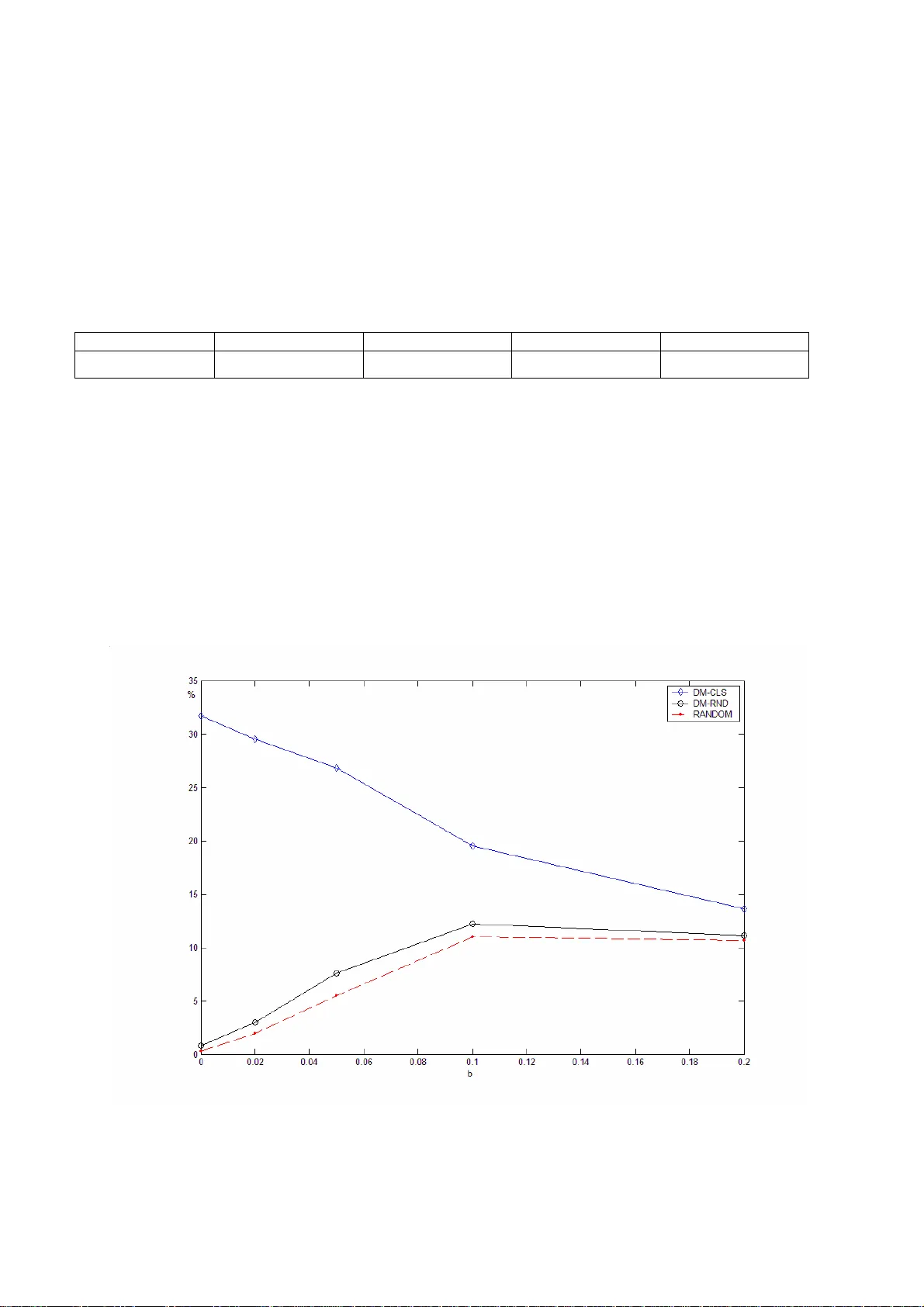
CLUSTER APPRO ACH TO THE DO MAINS FORMATIO N Leonid B. Litinskii Centre of Optical-Neural Technologies Scientific-Research Institute for System I nvestigates Russian Academy of Sciences CONT, Vavilov str., 44/2, Moscow, 1193 33, Russia litin@mail.ru Abstract. As a rule, a quadratic function al depending on a great numbe r of binary variables h as a lot of local minima. One of approaches allowing one to find in aver aged deeper local minima is aggregation of binary variables into larger blocks/dom ains. To minimize the functional one has t o change the states of ag gregated variable s (domains). In the present p ublication we discuss meth ods of domains f ormation. It is shown that the best results are obtained when domains are formed by variables that are strongly connected with ea ch other. Keywords: neural networ ks, minimiza tion problems, dynamical s ystems. 1. INTODUCTION W e discuss t he proble m of m inimization o f a quadrati c funct ional depen ding on binary v ariables : N {1 } i s =± () ( , ) m i n . i,j 1 N EJ s s ij i j =− =− ⎯ ⎯ → = ∑ sJ s s s ( 1 ) W ithout restricting the generality , we can suppose that the connection matrix is a symmetric one with zero elements on the m ain diagonal: W e m ake use of p hysical term inology [1]. In what follows the b inary variables will be called spins , N -dimensional vectors 1 () N ij J = J , JJ J ij ji ii = 0 . = {1 } i s =± 12 (, , . . . , ) N s ss = s will be called configuration vectors or configurat ions , and t he characteristic , which has to be minimized will be called the ener gy of the state . The commonly known pr ocedure of m inimi zation of the f unctional (1) is as f ollows: o ne random ly searches t hrough N spins, and to each spin the sign of the local field actin g on this spin is assigned: () E s s 1 () () . N ii j j ht J s t = = ∑ j ( 2 ) In other words, if the curre nt state of the spin () i s t coincides with the sign of (if the spin is satisfied : ), one does not change t he value of the spin: () i ht () () 0 ii st h t ≥ (1 ) ( ) ii s ts t + = ; but if () i s t and are of opposite signs (if the spin is unsatisfied : ), in the next moment of the time one turns th e spin over: () i ht () () 0 ii st h t < (1 ) ( ) ii s ts t + =− . It is well known that the energy of t he state decreases when an unsatis fied spi n turns over: . Sooner or later the system finds itself in the state, which is an energy minimum (may be this is a local minimum). In this state all the spins are satisfied and evolution of the system ends. In what follows the afor em entioned algorithm will be called the (( ) ) (( 1 ) ) Et Et >+ ss random dynamics (in the theory of neural networks it is called the asynchr onous dynamics [2]). Another wel l known m inimi zation proced ure is the synchr onou s dynamics , when each time all the unsatisfied sp ins turn over sim ultaneously [2] . This appr oach is rarely used in m ini mization problems. First, this is because in this case it is 2 impossible t o guarantee t he monoton ous decrease of the functional . Second, sy nchronous dynam ics is characterized by the presence of limit cycles of the leng th 2. Due to limit cycles the basin of attraction of local m inima decreases. () E s In the papers [ 3], [4] a ge nerali zation of rand om dynam ics, the domain dynam ics , was proposed. The essence of the generalization is joining the spins tog ether in larger blocks or, as they were called by the authors, doma ins . During the evolution n ot single spi n turns over, but the whol e block/dom ain. As for t he rest the dom ain approach i s the same as t he standard ra ndom dynamics. It was found t hat the dom ain dynam ics of fers a lot o f advantage s com paring with ot her dynamic approaches. The domain dynamics is times quicker than the ra ndom dy namics, whe re k is the averaged length of a doma in (the number of spins joi ned in one bl ock). More over , when using the dom ain dynam ics, the ener gy decreases monot onically , and it does not lead to l imit cycl es. Computer sim ulations with random Hebbian m atrices [4] showed that the dom ain dyna mics allowed one t o obtain de eper local mini ma of the funct ional (1) than t he standard ran dom dynamics. Ho wever , t here is an open quest ion: how one has to choose the dom ains to obtain the dee pest minim a? In the paper we discuss this question. 2 k () E s 2. DOMAIN DY NAMICS For simplicity of presentation all d efinitions are given for the case when the first k spins are joined in the 1s t domain, the k following spins are joined in the 2nd domain and so on. The last k spins are joined in the last n th domain: 11 2 ( 1 ) 1 1th domen 2 nd domen th domen ( , .. ., , , ... , , ... , , .. ., ). kk k n k N n s ss s s s +− + = s             ( 3 ) In Eq. (3) and s is an arbitrary configuration. Nk n = The total action onto the 1st domain from all other do mains is the superposition of all interactions of the spins, which do not belong to th e 1st domain, with th e spins of the 1st d omain. Then the local domain field actin g onto the i th spin belonging to the 1st domain is equal to () 11 () () () () , , Nk d ii j j i i j j jk j ht J s t h t J s t i k =+ = == − ∀ ∑∑ ≤ l ( 4 ) where is the local field (2). In other wo rds, the local domain field acting on the i th spin is obtained by means of elimination of the influ ence of the spins belonging to th e same domain from the local field (2). It is clear that the energy of interaction of the first domain with all other domains is equal to () i ht () i ht () 11 1 () () () () . k d ii i Et F t st h t = =− =− ∑ In the same way we define the local domain field acting onto th e spins belonging to the l th domai n, () (1 ) 1 () () () , ( 1 ) 1 , [ 2 , ] . lk d ii i j j jl k ht h t J s t l k i l k l n =− + =− ∀ − + ≤ ≤ ∈ ∑ The energy of interaction of the l th domain with other domains is: () (1 ) 1 () () () () , 2 , . . , . lk d ll i i il k Et F t st h t l n =− + =− =− = ∑ Then the domain energy of the state is () t s () 11 () () () . nn d l ll Et E t F t == == − ∑∑ ( 5 ) 3 The energy (1), which we have to minimize, differs from the domain energ y by the sum of the quantities that characterize the inter-domain interactions between spins only: () in l E () ( ) () 11 ( 1 ) 1 ( 1 ) 1 () () () () () () , n n lk lk di n d l ll i l k j l k E t Et E t Et J s t s t == = − + = − + =+ = − ∑∑ ∑ ∑ i j i j ( 6 ) After that we can define the domain dynamics [3],[4]: one random ly searches thro ugh n domains; if for the l th domain the inequality is fulfilled, the domain remains unchanged; but if () 0 l Ft ≥ () 0 l Ft < , in the next m oment one turns over th e l th domain – all the spins of the domain receive the opposite sings simultan eously: ( 1 ) ( ), [( 1 ) 1 , ]. ii s ts t i l k l += − ∈ − + k From Eq. (5) i t is easy to obtain that w hen using t he doma in dynamics, the dom ain ener gy of the state decreas es monotonical ly: if in the m oment t the m th domain is t urned over, the dom ain energy goe s down by t he value 4( ) m F t : () () (1 ) ( ) 4 ( ) dd m Et Et F t += − . Note, in the same time the energy E ( s ( t )) (1 ) that has to be m inimi zed, goes down just by the same value. This follows from Eq. (6) and the obv ious fact that simultaneous chan ge of the signs of all spin s belonging to the m th domain does not chan ge the inter-domain energy . () in m E As a result of the aforementioned proce dure so oner or later the system finds itself in the domain lo cal min imu m. I n t hi s state for all the domains the inequality is fulfilled, and the domain evolution end s. However, the local domain minimum is not necessarily a minimum of th e functional (1). That is why in this state one has “to defrost” the domains and use the standard random dynamics. The dynamic system has the possibility to descen d deeper into the minimum of the functional (1). () 0 l Ft ≥ The consecutive use of t he domain dy namics and than t he standard rand om dynami cs is based on the following argumentation. Minimization of th e functional (1) can be interp reted as the sliding of the dynamic system down a hillside that is dug up by shallow loca l minima . In the case of the random dynamics two consec utive states of the system di ffer by an opposite sign of only one binary coor dinate, na mely thos e that is tur ned over duri ng the give n step of e voluti on. It is evident that under th is dynamics the system sticks in th e fi rst occurring l ocal minim um. On the cont rary, under the do main dynamics t wo consecutive st ates of the syst em differ by opposite signs of some spin coordinates at once. The domain dynamics can be likeni ng to sliding do wn by more “large- scale steps”. It can be expect ed th at such way of motion al lows the system to leave aside a lot of shallow local minima, where it can stick in the case of random dynamics. As noted above, for simplicity we gave all th e definitions supposing that all the domains are of the same leng th k , and that spins joined in a domain have c onsecu tive numbers – see Eq.(3). It is evident th at in the general case dom ains can be of different lengths , and any spins can be joined in a domai n. In this connec tion the re are some questions: does the choice of the dom ains influence t he results of m inimi zation? How the d omains ha ve to be orga nized? Have t hey been inva riable for a given m atrix J , or have they bee n organized r andomly at every step of evolut ion? Generally , are there any argumentat ions, which can help? In the next sect ion we form ulate our reci pe of the dom ain formati on and present argument s proving it . In Section 4 we sh ow the results of com puter simul ation. l k Note. The idea of the domai n dynamics is so nat ural that, pr obably, it was p roposed more than once by differe nt authors. In partic ular, during preparing this publi cation we f ound out t hat the d omain dy namics is pract ically equivalent t o the block-sequential dynamics presented in [5]. We note that in [5] th e block-sequential dynamics was analyzed with regard to the proble m of increa sing the stora g e capacity of the Hopfield model. As fa r as we know, in [3], [4 ] the domain dynamics was used for m inimizati on of the f unctional (1 ) for the fi rst time. 4 3. CLUSTER APPROACH OF DO MAIN FORMATIO N 1. For the Hopfield model it is k nown the situation when do ma ins are naturally appeared due to specific properties of the Hebbian connection matrix J [6]. Let us cite the corresponding results, accentu ating the points we nee d. In the end of this Section we for mulate the reci pe of the d omain form ation in the gene ral case. Let us have N M -dimensional vector-col umns with bin ary coordi nates , , , i ∈ M xR () 1 i x μ =± 1 , ..., iN = 1 , .., . M μ = V ector -colum ns are numerated by subsc ripts i x [1, ] iN ∈ , and their coordi nates by supe rscripts [1, ] M μ ∈ . The relation between the di mension M of the vecto r-colum ns and their num ber N does not mean for our purpose. Let us construct ( M x N )-m atrix X , whose columns are M -dimensional vectors : i x (1) (1) (1 ) 12 (2) (2) (2) 12 () () () 12 ... ... . ... ... ... ... ... N N MM M N xx x xx x xx x ⎛⎞ ⎜⎟ ⎜⎟ = ⎜⎟ ⎜⎟ ⎜⎟ ⎝⎠ X In the theory of ne ural networks X is called the pattern matrix. It is used to c onstruct the Hebbia n matrix that is ( N x N )- matrix of scalar products of the vecto r-colum ns (and its diagonal elements are su pposed to be zeros): i x () () 1 (1 ) (1 ) (, ) , 1 , . M ij ij ij i j i j J xx i j N MM μμ μ δδ = −− == ≤ ∑ xx ≤ Since the lengths of the vector-colum ns are equal to i x M , the matrix elements of ij J are cosines of the angles between the corresponding vectors: || 1 ij J . ≤ We shall examine a special case, when the num ber of different vector-columns in the matrix X is not N , but a sm aller number n : . Then each vector-c olumn will be repeated some times. Let be the number of repetitions of the vector -column : . (The su bscripts l , m are used to numerate 1 ... .. ... .. , ln nN ≠≠ < xxx l x l k l x 1 n l kN = ∑ differen t vector-c olumns and related characteristics.) W it hout loss of ge nerality it can be assum ed that the first vector-columns of the matrix X coincide with each other , the next vector-colum ns coincide with each other , and so on; the last vector -columns coincide with each other too: 1 k 2 k n k 12 (1) (1) (1) (1) (1) (1) 11 22 (2) (2) ( 2 )( 2 ) ( 2 )( 2 ) 11 22 () ( ) () () () () 11 22 ... ... ... ... ... ... ... , 1. ... ... ... ... ... ... ... ... ... ... ... ... n nn nn l MM MM MM nn kk k xx xx xx xx xx xx k xx xx xx ⎛⎞ ⎜⎟ ⎜⎟ ⎜⎟ =≥ ⎜⎟ ⎜⎟ ⎜⎟ ⎜⎟ ⎝⎠ X                ( 7 ) The corresponding He bbian matrix consists of nn × blocks. The dimensionality of the ( lm )th block is equa l to () lm kk × , and all its elements are equal to the same num ber lm J that is the cosine of th e angle between the vectors and ( ). On the main diagonal there are quadratic ( l x m x , 1 , ..., lm n = ) ll kk × -blocks; these blocks c onsist of ones only (with the exception of the diagonal, where all the elements are equal to zero): 5 12 12 12 1 1 12 1 12 12 1 1 21 21 2 2 21 2 21 21 2 2 11 2 2 12 11 2 2 0 1 1 ... ... 1 1 ... 1 1 0 ... ... ... 0 1 1 ... 1 1 ... ... 1 1 0 ... ... ... 0 1 1 ... 1 ... ... n k kk nn n nn nn n nn nn n n nn nn n n JJ J J JJ JJ J J JJ J J JJ JJ J J JJ J J JJ JJ J J = J                %# ## # ## % # # ## % # ## # # ,1 , , [ 1 , 1 110 lm ] . J lm n ⎛⎞ ⎜⎟ ⎜⎟ ⎜⎟ ⎜⎟ ⎜⎟ ⎜⎟ ⎜⎟ <∈ ⎜⎟ ⎜⎟ ⎜⎟ ⎜⎟ ⎜⎟ ⎜⎟ ⎜⎟ ⎜⎟ ⎜⎟ ⎝⎠ % (8) It was found out [6] that such organizatio n of the connection m atrix imposes the form of the local minim a of the functional (1), namely: the local m inimum certa inly has the block-cons tant form 12 11 2 2 ( ... , ... , ..., ... ), 1 , 1 , . .., . n nn l kk k s ss s s s s l n = s             = ± = ( 9 ) In other words , the first coordinates o f the local minim u m have to be identical; the next coordinates have to be equal to each other , and so on. In Eq.(9) fragm entation into blocks of constant sig ns is defined by the block structure of the Hebbian matrix (or , and that is the same, by the stru cture of the repeating colu m ns in the pattern matrix X (7) ) . The proof that the local minim a have the block-constant form (9 ) is based on the fact that spi ns from one block ha ve the same connections with all other spins, and un de r the action of the local fields they behave in the sam e way (see item 1 of Appendi x). 1 k 2 k Not all configurations of the form (9) ar e t h e local minima of the functional (1), but it is necessary to look for the local minim a among these configurations only . In other words, for m i nimization of t h e functional (1), it is s enseless to examine configurations with dif ferent signs inside blocks of co nstant signs. It makes sense to examine confi gurations of the form (9) only . All spins from the same block are satisfied or not satis fied simultaneously . In the last case it is senseless to turn ov er unsatisfied spins from the block separately , because this lead s to a nonsensical configuratio n for which inside a block o f constant sign there are coordinates with di f ferent signs. It turned out , that in this case it is po ssible to turn over the whol e unsatisfied block sim ultaneously . This leads to a decrease of the energy ( 1). In other words, here the block s of the constant signs play the role of natural domains. 2. G enerally speaking, in this case the domains can be constructe d in a ra ndom way also, and after that they can be used for the dom ain minimization of the functional ( 1). In the experimental part of the prese n t work we tried to find out which way of the domain form ation leaded to better results. Howeve r , before describin g the experimental results, we would like to formulate the general rule of “ the correct domains” formation: Firstly , a domain consists of spins whose inter-connections ar e stronger , then their connec t ions with other spins . Secondly , the values of spins belon ging to th e same doma in have to be equa l. Due to evident relation of the general rule to the well known problem of the clustering of the symm etric matrix [7]-[9], this recipe will be called the cluster principle of the dom ains formation. In the clustering problem it is necessary to transform the sym metric matrix to a block-diagonal form, so that the matrix elements inside dia gonal blocks are greater than the elements outside the diagonal blocks. In the e n d of this paper we discuss this problem in details. 6 Justification of the cluster principle is rather obvious. The m atrix element ij J is considered as a measure of the connection between i th and j th spins. The validity of the cluster principle is base d on the fact that strongly connected spins have to interact with the rest of the spin s similarly . Therefor e, we have a go od ch ance that under action of an external field the strongly connected spins will behave themselves similarly . Concluding thi s Section, let us note that the above construc ted Hebbian matrix relates to a rather idealized situation, when the diagonal bl ocks of the matrix consist of ones. A ccording to Eq.(9), when constructing “correct dom ains” we combine into one dom ain those spins that are extremely strong connected with each ot he r . In practice such idealized situation can be found ve ry rarely . In our computer sim ulations we examined not this idealized case only , but more realistic Hebbian matrices too. 4. RESULTS OF COMPUTER SIMULATION 1. I n first series of th e computer experiments we used the Hebb ian matrices with extremely strong in ter-group connections (see the item 1 of the previous Section) . The e xternal parameters of th e problem were as follows: the dimensionality of the problem was N =1000, the number of patterns was M =60, the number of domains was n =40, sizes of domains were random num bers from the interval [1, 45]: ; the coordinates l k 40 1 1000 l l k = = ∑ () l x μ in the matrix (7) took on the values equiproba ble. 1 ± On the main diagonal of the He bb ian matrix (8) there were 40 () ll kk × -blocks from the ones only: () 1 in ll J = . Matrix elements outside these blocks were ra ndom quantities with th e mean values equal to 0 and the dispersions equal to 1/ M : , () 0 out lm J <> = () () 1 / out lm J M σ = . The cluster principle of the dom ains formation provides us with 40 domains of the type (9) generated b y 40 groups of stro ngly connected spins. Altogether 200 such a matrices J were generated, and for eac h matrix the functional (1) was minimized using 3 dynamic approaches: 1) RANDOM: the standard random dynamics was set going from 1000 rand om start configurations; 2) Random Domains (DM-RND) : the domain dynam ics was set going from the same random configurations with n =40 random domains of the ide ntical size k =25 (25 spins with random numbers were included in a d omain; inside a domain the spi ns had the values 1 ± equiprobabl e); 3) Cluster Domains (DM-CLS) : the domain d ynamics was set going from 1000 random start configurations of block- constant form (9). When a domain local m inimum was achieve d, the dom ains were “defrosted” and unde r the standard random dy namics the system went down to a deeper local minim u m of the functional (1). (N ote, in the case of cluster domains the domain local minima are local minima of the functional (1) too - s ee the ite m 2 of Appendix; in th is particular case the dom ain defrosting do es not allow the system to g o down deeper.) Thus, for each matrix we obtained 3000 local minim a. Then we found the deepest am ong them and calculated the frequency of the deepest minimum determination for each of the three dynam ics: RANDOM, DM-RND a nd DM-CLS. The dynamics, for which the frequency of the deepest local mi ni mum determination is the largest, has to be declared the best. In Fig.1 the results averaged over 20 0 random tests are show n for all the three dynam ics. Along the abscissa axis the three dynami cs are marked off, along the ordinate a xis we show the averaged freque ncy of the deepest mi nimum 7 determination (in percentage terms). It is seen that in aver age the domain dy namics with cluster domains (DM-CLS) leads to the deepest minimum more then 30 times frequently than the random domain dynamics (DM- RND) or the standard random dynamics (RANDOM ). Here the preference of th e cl uster domain formati on approach is evident. Fig.1. The average fre quency of the deepest mini mum determination for al l the three dynamics. 2. In the des cribed experiments the con n ections between s pins inside “the correct” groups were equal to ma xi mal value, because all vector-columns in one group were the sam e. What happens if these groups of vectors are slig htly “diluted”: If the vector-col umns inside “the correct” groups are not ide ntical, but differ sli ghtly? How this affects the resu lt of minim ization? l k l x The aforem entioned experiments were re peated for “diluted” gr oups of vector-col umns . In this case the first vector-colum ns of the matrix (7) were no t identical, but they were obtained as a result of mu ltiplicative distortion of the vector : with the probability b the coordinates of the vector (independently and randomly) were multiplied by -1. Analogously , the next vector-c olumns of the matrix X were obtained by m ultiplicativ e distortion of random vector , and so on. The last vector-colum ns of the matrix X were the result of mult iplicative distortion of random vector . l x 1 k 1 x 1 x 2 k 2 x n k n x Then the conn ections between spins inside “the correct” groups were random quantities with the mean values () 2 (1 2 ) in ij J b <> = − . Thus, the distortion probabil ity b characterized the level of inhom oge neity of “the correct” spin groups: the larger b, the less the mean va lue of the inter-group connection, the greater the inhomogeneity o f “the correct” gro up of spins. (As befo re the estimate of the connections between spins from different groups was () ~1 / out ij J M ± .) The values of b an d corresponding mean valu es of the inter-group connectio ns are given in T able 1. Note, only for b =0.02 and b = 0.05 “the correct” groups of spins ca n be regarded as strongly connected. Indeed , in these cases the mean values of the inter -group connections are and , respectively . In other words, the angles between M -dim ensional vectors x () 0.9 in ij J <> ≈ () 0.8 in ij J <> ≈ i from “the correct” groups a r e less than . Such groups of vector s still can be regarded 45 D 8 as compact, and the relative spins can be regarded as strongly connected. However , already for b =0.1 we have , and for b =0.2 the mean value of the inter- group connection becomes entirely small: . For such mean values of t he matrix elements, the groups we mechanically continue to consider as “co rrect” groups, in fact are aggregations of slightly connect ed spin sub-gr oups. The spins inside these sub-groups can be strongly connected, but in the same time the sub-groups are connected ra ther slightly . Note, when combining some slig htly connected sub-groups int o one large group, in fact we organize random dom ains. One might expect that the more b , the more the results for DM-C LS- dynamics resem ble the results for DM-RND-dy namics. () 0.64 in ij J <> = () 0.36 in ij J <> = Ta b l e 1 . The mean value of the inter-group conn ec tion between spins as function of the distortion level b . () in ij J <> b 0.02 0.05 0. 1 0.2 () in ij J <> 0.92 0.81 0.64 0. 36 In Fig.2 for all three types of the dynamics it is shown how the mean frequency of the deepest minimum determination depends on the param eter b . W e see that when b increases, the result s for the cl uster domain dynamics (DM-CLS) progressively less dif fer from the results for the random domain dy namics (DM-RND), particularly be ginning from b =0.1. It can be expected, si nce when b increases, “the co rrect” groups of spins resem ble the random domains p r ogressively . W e pay ones attention that the results of the random domain dy namics are only slightly better than the results of the standard rando m dynamics: for all values of b the DM-RND-plot is only slightly higher than the RANDOM-plot. Possible this can be explained by the fact that in our experim ents th e length of the random dom ains, k = 25, was far from optimal. In Ref. [4] the rand om domain dynami cs has been examined for diff erent lengths of domains. It was found out that the best results could be obtained when k =2. Fig.2. The mean freq uency of the deepest minimum detecting as function of the distortion param eter b for all the three dynamics. 9 3. After the dynamical system finds itself in the domain local minim um, one has to “defrost” the dom ains and to use the standard random dynamics. At that the system gets chan ce to decrease its ener gy still more getting into the local minimum of the functional ( 1). Suppose D is the value of the domain local minim um, and E is the depth of the fina l l oc al mini mu m; i t is evident that D < 0 and E ≤ D. Then d = D / E and r= ( E-D )/ E are relative quantities character izing which part of the depth of the local minim u m is due to the domain dynamics, and which part is due to the random dynamics: 0 ≤ d , r ≤ 1, d + r =1. If, for example, r ≈ 0, we conclude that practically all the depth of the local minimum is defined just by the contribution of the dom ain dynamics, and some increas e of the l o cal minimum depth due to the random dynamics is negligible. On the other hand, if r ≈ 1, the situation is reversed: th e dom ain dynamics does not influence significantly on the l ocal minimum depth, and t he random dynamics plays the main role. In fact, d and r characterize the relative contribution of the domain and random dynamics to the depth of t h e local mini m u m. It is interesting to compare the values of d - and r- characteristics for both varian ts of the domain dy namics. T o do this, we, at first, for each matrix averaged the r -characteristics over 1000 random starts, and then we averaged it over 200 rand om matrices. This has been done fo r two examined types of the domain dynamics . The plots of the averaged r -characteristics are shown in Fig.3. Here the distortion level b is along the abscissa axis, and r -characteristics for the cluster domain (DM -CLS) and random dom ain (DM-RND) dynam ics (averaged over 20000 0 starts) are along axis of ordinates. W e see that random domains give us r ≈ 1. In other words, when random d omains are used in av erage only 5% of the depth of the local mi nimum is defined by the contribution of the domain dynamics. The remaining 95% of the depth of the local minimum accounts for the standard random dynamics. This res ult is practically independent of the dist ortion level b (see the (DM-RND)-curve). The same as in the end of the previous item we can say that when random domains of the length k =25 are used t he result of standard random minimization is im proved only slightly . V ice versa, r <<1 when cluster domains are used. In this case the lar gest part of the depth of the local minimum is defined by the contribution of the domain dynam ics namely , an d the contribution of the random dynamics is com paratively small (see the (DM-CLS) -curve). In the absence of distortions ( b =0) the domain local m inima ar e just the minima of the functional (1) (see item 2 of Appendix); so, in this case the strict equality r = 0 is fulfilled. As far as b increases, the r - characteristics increases too. However , it happens rather slow ly . T he contribution of the domain dynam ics predominates in the entire examined interval of b . 5. Conclusions The obtained results are th e eviden ce of the pro ductivity of the cluster principle of do mains form ation. At that the number and the structure of domain s are defi ned as a result of the co nnection matrix clusteri ng. A tr ansformatio n of a matrix to the block-diagonal form when its matrix elem ents insi de the diagonal blocks are greater than outside these blocks is usually implied by matrix clustering. There are a lot of different approaches t o solution of the problem. A review of me thods of clustering can be found in [7]-[9]. The clusterization procedu r e propose d in [10] recomm ende d itself rather good for the correlation type connection matrices. They are the matrices whose elem ents are scalar products of a set of v ectors. During the time of the order of this procedure allows one not merely to choose com pact groups of vectors, but gain the un derstanding of which of 2 () ON 10 these groups ar e closer and which are farther to each other . This information is useful for domains formation. Up to now we failed to generalize the clusterization pr ocedure [10] onto conn ection matrices of the general (not obviou sly correlation) forms. Author is grateful to Artem Murashkin, who has d one comput er simulations for this paper. The work was done in the framework of the project «Inte llectual computer systems» (the program 2.45 ) under financial sup port of Russian Basic Research Foundation (g rant 06-01-00109). Fig.3. The averaged r -characteristics for the domain dynamics for cl uster (DM-CLS) and random (DM-RND) dom ains. APPENDIX 1. Let us show that when the connection matrix consists of the blocks (8), the lo cal minima of the functional (1) have the piecewise constant form (9). T o do this it is su fficient to prove, for example, that the first coordinates of the local minimum have to be equal to each othe r . Argumentation that ascertains this statem ent will be carried out for the first two coordinates. 1 k Suppose the configuration 123 ( , , , ..., ) N s ss s = s is a local minimum. Then each of the coordinates i s must have the same sign as the local field acting on this coordinate: 11 1 1 1 0 N jj j sh s J s = = ≥ ∑ and 22 2 2 1 0 N jj j sh s J s = = ≥ ∑ . Since the matrix J has the form (8), the local fields can be written as: and 12 hs H =+ 21 hs H = + . For both cases the second term 3 N ij j j H Js = = ∑ is the same, since all matrix elements of the first and th e second rows (with subscr ipts j >2) are the same: (see Eq.(8)). Thus t w o inequalities have to be fulfilled simultaneously: 12 , jj JJ j => 2 12 1 0 ss s H + ≥ and 21 2 0 ss sH + ≥ . If we su gge st t ha t t he coordinates 1 s and 2 s differ , then , and as a result we obtain 1 ≤ H and 1 ≤ - H . This is im possible. Consequently , 12 1 ss =− 11 our suggestion is incor r ect, and the coordinates 1 s and 2 s must coincide. This com pletes the proof that the local minima of the functional (1) with the matrix J (8) has the piecewise constant form (9). 2. It is easy to see that for t he block-constant Hebbian matrix (8) any conf iguration of the form (9) that is a dom ain local minimum is a local minimum of the functional (1) also . Indeed, suppose for the first domain the inequality is fulfilled. Since first coordinates 1 () 1 1 0 k d ii i Fs h = = ∑ ≥ 1 k i s (which just form the dom ain) are equal to each other, the sum in the right-hand side of the la st expression is t he sum of equal terms: 1 k () 11 d ii F ks h = . Consequently, If we use the expressi on (4) connecting the local field with the doma in local field , we obtain that the following expression is also positive: () 11 1 1 1 0. N d jj jk sh s J s =+ =≥ ∑ i h () d i h 1 () () 11 11 1 1 11 1 1 (1 ) k dd jj j sh sh s J s sh k = =+ =+ − > ∑ 0 . ( 1 0 ) This means that the sign of t he coordinate 1 s coincides with the sign of the local field , acting on this coordinate from the entire network. In other words, i n this case a domain local minim u m is also a local m inimum of the functional (1). It is interesting that the opposite is incorrect: from the piecewise constant form (9 ) being a l ocal minimum of the functional (1) it does not follow that it is a domain local minimum also . It can be easi ly seen from the expression (10): 1 h () 11 d s h can be negative, but if is sufficiently large, the sum in the right-hand side of Eq.(10) is positive. In other words, two inequalities are fulfilled simultaneously: , 1 k 11 0 sh > () 11 0 d sh < . By the way, from the last statement it follows that the dom ai n dynamics allows one to get out from sha llow local m ini ma of the functional (1). Refere nces [1] A.K. Hartmann, H. Rieger. Optimization Algo rithm s in Physics. Wile y-VCH, Ber lin (2001). [2] J. Hertz, A. Krogh, R . Palmer . Introduction to t h e Theory of Ne ural Computation. Addison-W esley , 1991. [3] B.V. Kryz hanovskii, B.M. Magomedov, an d A.L. Mikaelyan. A Domain M odel of a Neural Network. Doklady Mathematics, v. 71(2) (2005) pp. 3 10-314. [4] B. Kryzhanovsky , B. Ma gomedov . On the Probability of Finding Lo cal Minima in Optimization Problem s. Pr oceedings of IJCNN’2006 , p. 5882–5887, V ancouver : 2006. [5] A.V .M. Herz, C.M. Marcus. Distributed dynamics in n e ural networks. Phys. Rev . E47 (1993 ) pp. 21 55-2161. [6] L.B. Litinskii. Direct calculation of the stable points of a neural network. Theoretical and Mathematical Physics, 1994, v.101(3), pp. 1492-150 1. [7] R. Xu, D. Wunsh II. Survey of Cluster ing Algorithms. IE EE Tra nsactions on Neural Networks, v. 16(3) (2005) pp. 645-678. [8] T. Li, Sh. Zhu, M. Ogihara. Algorithm s for clustering high dimensional and distri bute d data. Intelligent Data Analysis v.7 (2003) pp. 305-326 . [9] P. Ar abie, L.J. Hubert, and G. De So ete (Eds.) Clustering and Classification. World Scientific, 199 6 . [10] L. Litinskii, D. Romanov. Neural network cl ustering based on distances between objects. In: St. Kollias, A. Stafylopatis, W. Duch, E. Oja (Eds.), “Ar tificial Neural Networks – ICANN 2006. 16h International Conference”, 2006, Proceedings, Part II, pp.437-443.