A Bayesian reassessment of nearest-neighbour classification

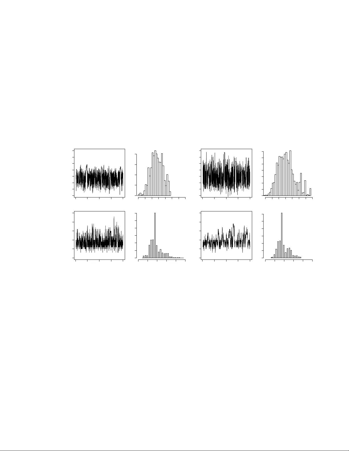
A Ba y esian reassessmen t of nearest–neigh b our classification Lionel Cucala 1 , Jean-Mic hel Marin 1 , 3 , Christian P . Rob ert 2 , 3 and D.M. Titterington 4 1 INRIA Sacla y , Pro jet select , Univ ersit´ e P aris-Sud, 2 CEREMADE, Univ ersit´ e P aris Dauphine, 3 CREST–INSEE, and 4 Univ ersity of Glasgo w Octob er 24, 2018 Abstract The k -nearest-neigh b our pro cedure is a well-kno wn deterministic method used in sup ervised classification. This paper prop oses a reassessmen t of this approac h as a statistical tec hnique deriv ed from a prop er probabilistic model; in par ticular, we mod- ify the assessment made in a previous analysis of this metho d undertak en by Holmes and Adams (2002, 2003), and ev aluated by Mano c ha and Girolami (2007), where the underlying probabilistic mo del is not completely well-defined. Once a clear proba- bilistic basis for the k -nearest-neighbour pro cedure is established, w e deriv e computa- tional tools for conducting Ba yesian inference on the parameters of the corresp onding mo del. In particular, we assess the difficulties inherent to pseudo-likelihoo d and to path sampling approximations of an intractable normalising constant, and propose a perfect sampling strategy to implemen t a correct MCMC sampler asso ciated with our mo del. If p erfect sampling is not av ailable, w e suggest using a Gibbs sampling appro ximation. Illustrations of the performance of the corresp onding Ba yesian clas- sifier are provided for several benchmark datasets, demonstrating in particular the limitations of the pseudo-likelihoo d appro ximation in this set-up. Keyw ords: Ba yesian inference, classification, compatible conditionals, Boltzmann mo del, normalising constan t, pseudo-lik eliho o d, path sampling, p erfect sampling, MCMC algorithm. 1 In tro duction 1.1 Deterministic v ersus statistical classification Sup ervised classification has long b een used in b oth Machine Learning and Statistics to infer ab out the functional connection b et ween a group of cov ariates (or explanatory 1 v ariables) and a v ector of indicators (or classes) (see, e.g., McLac hlan, 1992; Ripley, 1994, 1996; Devro ye et al., 1996; Hastie et al., 2001). F or instance, the metho d of b o osting (F reund and Sc hapire, 1997) has b een dev elop ed for this very purp ose b y the Machine Learning communit y and has also b een assessed and extended by statisticians (Hastie et al., 2001; B ¨ uhlmann and Y u, 2002, 2003; B ¨ uhlmann, 2004; Zhang and Y u, 2005). The k -nearest-neigh b our metho d is a w ell-established and straightforw ard tec hnique in this area with b oth a long past and a fairly resilient resistance to c hange (Ripley, 1994, 1996). Nonetheless, while providing an instrument for classifying points into t wo or more classes, it lacks a corresp onding assessment of its classification error. While alternative tec hniques like b oosting offer this assessmen t, it is obviously of in terest to pro vide the original k -nearest-neigh b our metho d with this additional feature. In contrast, statistical classification metho ds that are based on a mo del suc h a mixture of distributions do pro- vide an assessment of error along with the most lik ely classification. This more global p erspective thus requires the technique to b e em b edded within a probabilistic frame- w ork in order to give a prop er meaning to the notion of classification error. Holmes and Adams (2002) prop ose a Bay esian analysis of the k -nearest-neigh b our-method based on these premises, and we refer the reader to this pap er for bac kground and references. In a separate pap er, Holmes and Adams (2003) defined another mo del based on autologis- tic representations and conducted a lik eliho o d analysis of this mo del, in particular for selecting the v alue of k . While we also adopt a Bay esian approac h, our paper differs from Holmes and Adams (2002) in t wo imp ortan t resp ects: first, w e define a global prob- abilistic mo del that encapsulates the k -nearest-neigh b our metho d, rather than working with incompatible conditional distributions, and, second, we deriv e a fully op erational sim ulation technique adapted to our model and based either on p erfect sampling or on a Gibbs sampling appro ximation, that allo ws for a reassessmen t of the pseudo-lik eliho o d appro ximation often used in those settings. 1.2 The original k -nearest-neigh b our metho d Giv en a training set of individuals allo cated each to one of G classes, the classical k - nearest-neigh b our pro cedure is a method that allocates new individuals to the most com- mon class in their neigh b ourho od among the training set, the neigh b ourho od b eing defined in terms of the co v ariates. More formally , based on a training dataset (( y i , x i )) n i =1 , where y i ∈ { 1 , . . . , G } denotes the class label of the i th p oin t and x i ∈ R p is a v ector of co v ari- ates, an unobserv ed class y n +1 asso ciated with a new set of co v ariates x n +1 is estimated b y the most common class among the k nearest neighbours of x n +1 in the training set ( x i ) n i =1 . The neighbourho o d is defined in the space of the cov ariates x i , namely N k n +1 =  1 ≤ i ≤ n ; d ( x i , x n +1 ) ≤ d ( · , x n +1 ) ( k )  , 2 where d ( · , x n +1 ) denotes the v ector of distances to x n +1 and d ( · , x n +1 ) ( k ) denotes the k th order statistic. The original k -nearest-neighbour metho d usually uses the Euclidean norm, ev en though the Mahalanobis distance w ould be more appropriate in that it rescales the cov ariates. Whenev er ties o ccur, they are resolved by decreasing the num b er k of neigh b ours un til the problem disappears. When some cov ariates are categorical, other t yp es of distance can b e used instead, as in the R pac k age knncat of Buttrey (1998). As suc h, and as also noted in Holmes and Adams (2002), the m ethod is b oth deter- ministic, giv en the training dataset, and not parameterised, ev en though the c hoice of k is b oth non-trivial and relev ant to the performance of the m ethod. Usually , k is selected via cross-v alidation, as the n umber of neigh b ours that minimises the cross-v alidation error rate. In contrast to cluster-analysis set-ups, the num b er G of classes in the k -nearest- neigh b our pro cedure is fixed and given by the training set: the introduction of additional classes that are not observ ed in the training set has no effect on the future allocations. ● ● ● ● ● ● ● ● ● ● ● ● ● ● ● ● ● ● ● ● ● ● ● ● ● ● ● ● ● ● ● ● ● ● ● ● ● ● ● ● ● ● ● ● ● ● ● ● ● ● ● ● ● ● ● ● ● ● ● ● ● ● ● ● ● ● ● ● ● ● ● ● ● ● ● ● ● ● ● ● ● ● ● ● ● ● ● ● ● ● ● ● ● ● ● ● ● ● ● ● ● ● ● ● ● ● ● ● ● ● ● ● ● ● ● ● ● ● ● ● ● ● ● ● ● ● ● ● ● ● ● ● ● ● ● ● ● ● ● ● ● ● ● ● ● ● ● ● ● ● ● ● ● ● ● ● ● ● ● ● ● ● ● ● ● ● ● ● ● ● ● ● ● ● ● ● ● ● ● ● ● ● ● ● ● ● ● ● ● ● ● ● ● ● ● ● ● ● ● ● ● ● ● ● ● ● ● ● ● ● ● ● ● ● ● ● ● ● ● ● ● ● ● ● ● ● ● ● ● ● ● ● ● ● ● ● ● ● ● ● ● ● ● ● ● ● ● ● ● ● −1.0 −0.5 0.0 0.5 1.0 −0.2 0.2 0.6 1.0 ● ● ● ● ● ● ● ● ● ● ● ● ● ● ● ● ● ● ● ● ● ● ● ● ● ● ● ● ● ● ● ● ● ● ● ● ● ● ● ● ● ● ● ● ● ● ● ● ● ● ● ● ● ● ● ● ● ● ● ● ● ● ● ● ● ● ● ● ● ● ● ● ● ● ● ● ● ● ● ● ● ● ● ● ● ● ● ● ● ● ● ● ● ● ● ● ● ● ● ● ● ● ● ● ● ● ● ● ● ● ● ● ● ● ● ● ● ● ● ● ● ● ● ● ● ● ● ● ● ● ● ● ● ● ● ● ● ● ● ● ● ● ● ● ● ● ● ● ● ● ● ● ● ● ● ● ● ● ● ● ● ● ● ● ● ● ● ● ● ● ● ● ● ● ● ● ● ● ● ● ● ● ● ● ● ● ● ● ● ● ● ● ● ● ● ● ● ● ● ● ● ● ● ● ● ● ● ● ● ● ● ● ● ● ● ● ● ● ● ● ● ● ● ● ● ● ● ● ● ● ● ● ● ● ● ● ● ● ● ● ● ● ● ● ● ● ● ● ● ● ● ● ● ● ● ● ● ● ● ● ● ● ● ● ● ● ● ● ● ● ● ● ● ● ● ● ● ● ● ● ● ● ● ● ● ● ● ● ● ● ● ● ● ● ● ● ● ● ● ● ● ● ● ● ● ● ● ● ● ● ● ● ● ● ● ● ● ● ● ● ● ● ● ● ● ● ● ● ● ● ● ● ● ● ● ● ● ● ● ● ● ● ● ● ● ● ● ● ● ● ● ● ● ● ● ● ● ● ● ● ● ● ● ● ● ● ● ● ● ● ● ● ● ● ● ● ● ● ● ● ● ● ● ● ● ● ● ● ● ● ● ● ● ● ● ● ● ● ● ● ● ● ● ● ● ● ● ● ● ● ● ● ● ● ● ● ● ● ● ● ● ● ● ● ● ● ● ● ● ● ● ● ● ● ● ● ● ● ● ● ● ● ● ● ● ● ● ● ● ● ● ● ● ● ● ● ● ● ● ● ● ● ● ● ● ● ● ● ● ● ● ● ● ● ● ● ● ● ● ● ● ● ● ● ● ● ● ● ● ● ● ● ● ● ● ● ● ● ● ● ● ● ● ● ● ● ● ● ● ● ● ● ● ● ● ● ● ● ● ● ● ● ● ● ● ● ● ● ● ● ● ● ● ● ● ● ● ● ● ● ● ● ● ● ● ● ● ● ● ● ● ● ● ● ● ● ● ● ● ● ● ● ● ● ● ● ● ● ● ● ● ● ● ● ● ● ● ● ● ● ● ● ● ● ● ● ● ● ● ● ● ● ● ● ● ● ● ● ● ● ● ● ● ● ● ● ● ● ● ● ● ● ● ● ● ● ● ● ● ● ● ● ● ● ● ● ● ● ● ● ● ● ● ● ● ● ● ● ● ● ● ● ● ● ● ● ● ● ● ● ● ● ● ● ● ● ● ● ● ● ● ● ● ● ● ● ● ● ● ● ● ● ● ● ● ● ● ● ● ● ● ● ● ● ● ● ● ● ● ● ● ● ● ● ● ● ● ● ● ● ● ● ● ● ● ● ● ● ● ● ● ● ● ● ● ● ● ● ● ● ● ● ● ● ● ● ● ● ● ● ● ● ● ● ● ● ● ● ● ● ● ● ● ● ● ● ● ● ● ● ● ● ● ● ● ● ● ● ● ● ● ● ● ● ● ● ● ● ● ● ● ● ● ● ● ● ● ● ● ● ● ● ● ● ● ● ● ● ● ● ● ● ● ● ● ● ● ● ● ● ● ● ● ● ● ● ● ● ● ● ● ● ● ● ● ● ● ● ● ● ● ● ● ● ● ● ● ● ● ● ● ● ● ● ● ● ● ● ● ● ● ● ● ● ● ● ● ● ● ● ● ● ● ● ● ● ● ● ● ● ● ● ● ● ● ● ● ● ● ● ● ● ● ● ● ● ● ● ● ● ● ● ● ● ● ● ● ● ● ● ● ● ● ● ● ● ● ● ● ● ● ● ● ● ● ● ● ● ● ● ● ● ● ● ● ● ● ● ● ● ● ● ● ● ● ● ● ● ● ● ● ● ● ● ● ● ● ● ● ● ● ● ● ● ● ● ● ● ● ● ● ● ● ● ● ● ● ● ● ● ● ● ● ● ● ● ● ● ● ● ● ● ● ● ● ● ● ● ● ● ● ● ● ● ● ● ● ● ● ● ● ● ● ● ● ● ● ● ● ● ● ● ● ● ● ● ● ● ● ● ● ● ● ● ● ● ● ● ● ● ● ● ● ● ● ● ● ● ● ● ● ● ● ● ● ● ● ● ● ● ● ● ● ● ● ● ● ● ● ● ● ● ● ● ● ● ● ● ● ● ● ● ● ● ● ● ● ● ● ● ● ● ● ● ● ● ● ● ● ● ● ● ● ● ● ● ● ● ● ● ● ● ● ● ● ● ● ● ● ● ● ● ● ● ● ● ● ● ● ● ● ● ● ● ● ● ● ● ● ● ● ● ● ● ● −1.0 −0.5 0.0 0.5 1.0 −0.2 0.2 0.6 1.0 ● ● ● ● ● ● ● ● ● ● ● ● ● ● ● ● ● ● ● ● ● ● ● ● ● ● ● ● ● ● ● ● ● ● ● ● ● ● ● ● ● ● ● ● ● ● ● ● ● ● ● ● ● ● ● ● ● ● ● ● ● ● ● ● ● ● ● ● ● ● ● ● ● ● ● ● ● ● ● ● ● ● ● ● ● ● ● ● ● ● ● ● ● ● ● ● ● ● ● ● ● ● ● ● ● ● ● ● ● ● ● ● ● ● ● ● ● ● ● ● ● ● ● ● ● ● ● ● ● ● ● ● ● ● ● ● ● ● ● ● ● ● ● ● ● ● ● ● ● ● ● ● ● ● ● ● ● ● ● ● ● ● ● ● ● ● ● ● ● ● ● ● ● ● ● ● ● ● ● ● ● ● ● ● ● ● ● ● ● ● ● ● ● ● ● ● ● ● ● ● ● ● ● ● ● ● ● ● ● ● ● ● ● ● ● ● ● ● ● ● ● ● ● ● ● ● ● ● ● ● ● ● ● ● ● ● ● ● ● ● ● ● ● ● ● ● ● ● ● ● ● ● ● ● ● ● ● ● ● ● ● ● ● ● ● ● ● ● ● ● ● ● ● ● ● ● ● ● ● ● ● ● ● ● ● ● ● ● ● ● ● ● ● ● ● ● ● ● ● ● ● ● ● ● ● ● ● ● ● ● ● ● ● ● ● ● ● ● ● ● ● ● ● ● ● ● ● ● ● ● ● ● ● ● ● ● ● ● ● ● ● ● ● ● ● ● ● ● ● ● ● ● ● ● ● ● ● ● ● ● ● ● ● ● ● ● ● ● ● ● ● ● ● ● ● ● ● ● ● ● ● ● ● ● ● ● ● ● ● ● ● ● ● ● ● ● ● ● ● ● ● ● ● ● ● ● ● ● ● ● ● ● ● ● ● ● ● ● ● ● ● ● ● ● ● ● ● ● ● ● ● ● ● ● ● ● ● ● ● ● ● ● ● ● ● ● ● ● ● ● ● ● ● ● ● ● ● ● ● ● ● ● ● ● ● ● ● ● ● ● ● ● ● ● ● ● ● ● ● ● ● ● ● ● ● ● ● ● ● ● ● ● ● ● ● ● ● ● ● ● Figure 1: T raining (top) and test (b ottom) groups for Ripley’s b enc hmark: the points in red are those for whic h the lab el is equal to 1 and the points in blac k are those for whic h the lab el is equal to 2. T o illustrate the original metho d and to compare it later with our approach, we use throughout a toy benchmark dataset taken from Ripley (1994). This dataset corresp onds to a tw o-class classification problem in which each (sub)p opulation of cov ariates is sim- ulated from a biv ariate normal distribution, b oth populations b eing of equal sizes. A sample of n = 250 individuals is used as the training set and the mo del is tested on a second group of m = 1 , 000 p oin ts acting as a test dataset. Figure 1 presents the dataset 1 1 This dataset is a v ailable at http://www.stats.o x.ac.uk/pub/PRNN . 3 and T able 1 displays the p erformance of the standard k -nearest-neigh b our metho d on the test dataset for several v alues of k . The ov erall misclassification lea ve-one-out error rate on the training dataset as k v aries is provided in Figure 2 and it sho ws that this criterion is not very discriminating for this dataset, with little v ariation for a wide range of v alues of k and with sev eral v alues of k ac hieving the same o verall minimum, namely 17, 18, 35, 36, 45, 46, 51, 52, 53 and 54. There are therefore ten differen t v alues of k in comp etition. This range of v alues is an indicator of p oten tial gains when a veraging o ver k , and hence calls for a Bay esian p ersp ectiv e. k Misclassification error rate 1 0.150 3 0.134 15 0.095 17 0.087 31 0.084 54 0.081 T able 1: k -nearest-neighbour p erformances on the Ripley test dataset 0 20 40 60 80 100 120 30 40 50 60 k Leave−one−out cross validation error rate Figure 2: Misclassification lea ve-one-out error rate as a function of k for Ripley’s training dataset. 4 1.3 Goal and plan As presented ab ov e, the k -nearest-neigh b our metho d is merely an allo cation technique that does not account for uncertaint y . In order to add this feature, we need to introduce a probabilistic framework that relates the class lab el y i to both the co v ariates x i and the class labels of the neighbours of x i . Not only do es this p ersp ectiv e pro vide more infor- mation ab out the v ariabilit y of the classification, when compared with the point estimate giv en by the original metho d, but it also takes adv antage of the full (Bay esian) inferen- tial mac hinery to in tro duce parameters that measure the strength of the influence of the neigh b ours, and to analyse the role of the v ariables, of the metric used, of the n umber k of neigh b ours, and of the num b er of classes to wards ac hieving higher efficiency . Once again, this statistical viewp oin t was previously adopted by Holmes and Adams (2002, 2003) and w e follo w suit in this pap er, with a mo dification of their original model geared to wards a coheren t probabilistic mo del, while providing new developmen ts in computational mo del estimation. In order to illustrate the app eal of adopting a probabilistic p ersp ectiv e, w e pro vide in Figure 3 t wo graphs that are b y-pro ducts of our Bay esian analysis. F or Ripley’s dataset, the first graph (on the left) giv es the level sets of the predictive probabilities to b e in the black class, while the second graph (on the righ t) partitions the square in to three zones, namely sure allocation to the red class, sure allo cation to the blac k class and an uncertain ty zone. Those three sets are obtained by first computing 95% credible interv als for the predictive probabilities and then chec king those interv als against the b orderline v alue 0 . 5. If the in terv al contains 0 . 5, the p oin t is ranked as uncertain. The paper is organised as follo ws. W e establish the v alidit y of the new probabilistic k - nearest-neigh b our mo del in Section 2, p oin ting out the deficiencies of the models adv anced b y Holmes and Adams (2002, 2003), and then co ver the different aspects of running Ba yesian inference in this k -nearest-neigh b our mo del in Section 3, addressing in particular the sp ecific issue of ev aluating the normalising constant of the probabilistic k -nearest- neigh b our mo del that is necessary for inferring ab out k and an additional parameter. W e tak e adv antage of an exact MCMC approach proposed in Section 3.4 to ev aluate the limitations of the pseudo-lik eliho o d alternativ e in Section 3.5 and illustrate the metho d on several benchmark datasets in Section 4. 2 The probabilistic k -nearest-neigh b our mo del 2.1 Mark o v random field mo delling In order to build a probabilistic structure that repro duces the features of the original k -nearest-neigh b our pro cedure and then to estimate its unkno wn parameters, we first need to define a joint distribution of the lab els y i conditional on the cov ariates x i , for 5 −1.0 −0.5 0.0 0.5 1.0 −0.2 0.0 0.2 0.4 0.6 0.8 1.0 xp yp −1.0 −0.5 0.0 0.5 −0.2 0.0 0.2 0.4 0.6 0.8 1.0 xp yp Figure 3: (left) Lev el sets of the predictive probabilit y to b e in the black class, ranging from high (white) to lo w (r e d) , and (right) consequences of the comparison with 0 . 5 of the 95% credibilit y interv als for the predictiv e probabilities. (These plots are based on an MCMC sample whose deriv ation is explained in Section 3.4.) the training dataset. A natural approac h is to take adv antage of the spatial structure of the problem and to use a Mark ov random field mo del. Although w e will sho w below that this is not p ossible within a coherent probabilistic setting, w e could th us assume that the full conditional distribution of y i giv en y − i = ( y 1 , . . . , y i − 1 , y i +1 , . . . , y n ) and the x i ’s only dep ends on the k nearest neighbours of x i in the training set. The parameterised structure of this conditional distribution is ob viously op en but w e opt for the most standard c hoice, namely , lik e the P otts model, a Boltzmann distribution (Møller and W aagep etersen, 2003) with p oten tial function X ` ∼ k i δ y i ( y ` ) , where ` ∼ k i means that the summation is taken o ver the observ ations x ` b elonging to the k nearest neighbours of x i , and δ a ( b ) denotes the Dirac function. This function actually gives the num b er of points from the same class y i as the p oint x i that are among the k nearest neigh b ours of x i . As in Holmes and Adams (2003), the expression for the full conditional is thus f ( y i | y − i , X , β , k ) = exp   β X ` ∼ k i δ y i ( y ` )  k   , G X g =1 exp   β X ` ∼ k i δ g ( y ` )  k   (1) where β > 0 and X is the ( p, n ) matrix { x 1 , . . . , x n } of co ordinates for the training set. 6 In this parameterised mo del, β is a quan tity that is ob viously missing from the orig- inal k -nearest-neigh b our pro cedure. It is only relev ant from a statistical p oin t of view as a degree of uncertain ty: β = 0 corresp onds to a uniform distribution ov er all classes, meaning indep endence from the neigh b ours, while β = + ∞ leads to a p oin t mass distri- bution at the prev alen t class, corresponding to extreme dep endence. The in tro duction of the scale parameter k in the denominator is useful in making β dimensionless. There is, how ev er, a difficulty with this expression in that, for almost all datasets X , there do es not exist a joint probability distribution on y = ( y 1 , . . . , y n ) with full conditionals equal to (1). This happens because the k -nearest-neigh b our system is usually asymmetric: when x i is one of the k nearest neighbours of x j , x j is not necessarily one of the k nearest neighbours of x i . Therefore, the pseudo-conditional distribution (1) will not dep end on x j while the equiv alent for x j do es depend on x i : this is ob viously imp ossible in a coherent probabilistic framew ork (Besag, 1974; Cressie, 1993) One wa y of o vercoming this fundamental difficulty is to follow Holmes and Adams (2002) and to define directly the joint distribution f ( y | X , β , k ) = n Y i =1 exp   β X ` ∼ k i δ y i ( y ` )  k   , G X g =1 exp   β X ` ∼ k i δ g ( y ` )  k   . (2) Unfortunately , there are dra wbacks to this approach, in that, first, the function (2) is not prop erly normalised (a fact o verlooked b y Holmes and Adams, 2002), and the necessary normalising constan t is in tractable. Second, the full conditional distributions correspond- ing to this join t distribution are not given by (1). The first dra wback is a common o ccur- rence with Boltzmann mo dels and we will deal with this difficult y in detail in Section 3. A t this stage, let us p oint out that the most standard approac h to this problem is to use pseudo-lik eliho o d following Besag et al. (1991), as in Heikkinen and Hogmander (1994) and Ho eting et al. (1999), but we will show in Section 3.5 that this appro ximation can giv e p oor results. (See, e.g., F riel et al. (2005) for a discussion of this point.) The second and more sp ecific dra wback implies that (2) cannot be treated as a pseudo-lik eliho od (Besag, 1974; Besag et al., 1991)since, as stated ab o ve, the conditional distribution (1) cannot be asso ciated with any joint distribution. That (2) misses a normalising constan t 7 can b e seen from the special case in which n = 2, y = ( y 1 , y 2 ) and G = 2, since 2 X y 1 =1 2 X y 2 =1 2 Y i =1 exp   β X ` ∼ k i δ y i ( y ` )  k   , 2 X g =1 exp   β X ` ∼ k i δ g ( y ` )  k   = 2 X y 1 =1 2 X y 2 =1 exp ( β [ δ y 1 ( y 2 ) + δ y 2 ( y 1 )] /k ) ,  1 + e β /k  2 = 2  1 + e 2 β /k    1 + e β /k  2 , whic h is clearly different from 1 and, more imp ortan tly , dep ends on b oth β and k . W e note that the debate ab out whether or not one should use a prop er join t distribution is reminiscen t of the opp osition b et w een Gaussian conditional autoregressions (CAR) and Gaussian intrinsic autoregressions in Besag and Ko operb erg (1995), the latter not being asso ciated with an y joint distribution. 2.2 A symmetrised Boltzmann mo delling Giv en these difficulties, we therefore adopt a different strategy and define a joint mo del on the training set as f ( y | X , β , k ) = exp   β n X i =1 X ` ∼ k i δ y i ( y ` )  k   , Z ( β , k ) , (3) where Z ( β , k ) is the normalising constant of the distribution. The motiv ation for this mo delling is that the full conditional distributions corresp onding to (3) can b e obtained as f ( y i | y − i , X , β , k ) ∝ exp    β /k   X ` ∼ k i δ y i ( y ` ) + X i ∼ k ` δ y ` ( y i )      , (4) where i ∼ k ` means that the summation is tak en ov er the observ ations x ` for whic h x i is a k -nearest neigh b our. Ob viously , these conditional distributions differ from (1) if only b ecause of the impossibility result men tioned ab ov e. The additional term in the p oten tial function corresp onds to the observ ations that are not among the nearest neigh b ours of x i but for which x i is a neares t neighbour. In this model, compared with single neighbours, m utual neigh b ours are given a double w eight. This feature is of imp ortance in that this coheren t mo del defines a new classification criterion that can b e treated as a comp etitor of the standard k -nearest-neigh b our ob jectiv e function. Note also that the original full conditional (1) is reco vered as (4) when the system of neighbours is p erfectly symmetric 8 (up to a factor 2). Once again, the normalising constan t Z ( β , k ) is intractable, except for the most trivial cases. In the case of unbalanced sampling, that is, if the marginal probabilities p 1 = P ( y = 1) , . . . , p G = P ( y = G ) are known and are differen t from the sampling probabilities ˜ p 1 = n 1 /n, . . . , ˜ p G = n G /n , where n g is the num b er of training observ ations arising from class g , a natural mo dification of this k -nearest-neigh b our mo del is to reweigh t the neigh b ourho od sizes b y a g = p g n/n g . This leads to the mo dified mo del f ( y | X , β , k ) = exp   β X i a y i X ` ∼ k i δ y i ( y ` )  k   , Z ( β , k ) . This mo dification is useful in practice when we are dealing with stratified surveys. In the follo wing, how ever, w e assume that a g = 1 for all g = 1 , . . . , G . 2.3 Predictiv e p ersp ectiv e When based on the conditional expression (4), the predictive distribution of a new un- classified observ ation y n +1 giv en its co v ariate x n +1 and the training sample ( y , X ) is, for g = 1 , . . . , G, P ( y n +1 = g | x n +1 , y , X , β , k ) ∝ exp    β /k   X ` ∼ k ( n +1) δ g ( y ` ) + X ( n +1) ∼ k ` δ y ` ( g )      , (5) where X ` ∼ k ( n +1) δ g ( y ` ) and X ( n +1) ∼ k ` δ y ` ( g ) are the num b ers of observ ations in the training dataset from class g among the k nearest neigh b ours of x n +1 and among the observ ations for whic h x n +1 is a k -nearest neigh- b our, resp ectively . This predictiv e distribution can then b e incorp orated in the Bay esian inference pro cess b y considering the join t p osterior of ( β , k , y n +1 ) and by deriving the corresp onding marginal p osterior distribution of y n +1 . While this mo del pro vides a sound statistical basis for the k -nearest-neighour method- ology as w ell as a means of assessing the uncertain ty of the allocations to classes of unclassified observ ations, and while it corresp onds to a true, alb eit unav ailable, join t dis- tribution, it can b e criticised from a Ba yesian p oint of view in that it suffers from a lac k of statistical coherence (in the sense that the information contained in the sample is not used in the most efficien t wa y) when m ultiple classifications are considered. Indeed, the k -nearest-neigh b our metho dology is in v ariably used in a rep eated manner, either jointly on a sample ( x n +1 , . . . , x n + m ) or sequen tially . Rather than assuming sim ultaneously de- p endence in the training sample and indep endence in the unclassified sample, it would 9 b e more sensible to consider the whole collection of p oints as issuing from a single joint mo del of the form given by (3), but with some having their class missing at random. Alw ays reasoning from a Ba yesian p oin t of view, addressing join tly the inference on the parameters ( β , k ) and on the missing classes ( y n +1 , . . . , y n + m )—i.e. assuming exchange- ability b et ween the training and the unclassified datapoints—certainly makes sense from a foundational p erspective as a correct probabilistic ev aluation and it do es provide a b etter assessmen t of the uncertain ty ab out the classifications as well as ab out the parameters. Unfortunately , this more global and arguably more coheren t persp ective is mostly unac hiev able if only for computational reasons, since the set of the missing class vector ( y n +1 , . . . , y n + m ) is of size G m . It is practically impossible to derive an efficien t sim ulation algorithm that w ould correctly approximate the joint probability distribution of b oth parameters and classes, especially when the n umber m of unclassified p oints is large. W e will thus adopt the more ad ho c approach of dealing separately with eac h unclassified p oin t in the analysis, because this simply is the only realistic wa y . This p erspective can also b e justified b y the fact that, in realistic machine learning set-ups, the unclassified data ( y n +1 , . . . , y n + m ) mostly o ccur in a sequential en vironment with, furthermore, the true v alue of y n +1 b eing rev ealed b efore y n +2 is observed. In the follo wing sections, w e mainly consider the case G = 2 as in Holmes and Adams (2003), because this is the only case where we can conduct a full comparison b et ween differen t approximation sc hemes, but we indicate at the end of Section 3.4 how a Gibbs sampling appro ximation allo ws for a realistic extension to larger v alues of G , as illustrated in Section 4. 3 Ba y esian inference and the normalisation problem Giv en the joint mo del (3) for ( y 1 , . . . , y n +1 ), Bay esian inference can b e conducted in a standard manner (Rob ert, 2001), provided computational difficulties related to the un- a v ailabilit y of the normalising constan t can be solv ed. Indeed, as stressed in the previous section, from a Ba yesian p erspective, the classification of unclassified p oints can b e based on the marginal predictiv e (or posterior) distribution of y n +1 obtained b y in tegration o v er the conditional p osterior distribution of the parameters, namely , for g = 1 , 2 , P ( y n +1 = g | x n +1 , y , X ) = X k Z P ( y n +1 = g | x n +1 , y , X , β , k ) π ( β , k | y , X ) d β , (6) where π ( β , k | y , X ) ∝ f ( y | X , β , k ) π ( β , k ) is the p osterior distribution of ( β , k ) giv en the training dataset ( y , X ). While other choices of prior distributions are av ailable, w e c ho ose for ( k , β ) a uniform prior on the compact supp ort { 1 , . . . , K } × [0 , β max ]. The limitation on k is imp osed b y the structure of the training dataset in that K is at most equal to the minimal class size, min( n 1 , n 2 ), while the limitation on β , β < β max , is customary 10 in Boltzmann mo dels, b ecause of phase-transition phenomena (Møller, 2003): when β is ab o ve a certain v alue, the mo del b ecomes ”all blac k or all white”, i.e. all y i ’s are either equal to 1 or to 2. (This is illustrated in Figure 5 below b y the conv ergence of the exp ectation of the num b er of iden tical neigh b ours to k .) The determination of β max is obviously problem-sp ecific and needs to b e solved afresh for eac h new dataset since it dep ends on the top ology of the neighbourho o d. It is how ever straighforw ard to implemen t in that a Gibbs simulation of (3) for differen t v alues of β quic kly exhibits the “blac k-or-white” features. 3.1 MCMC steps W ere the p osterior distribution π ( β , k | y , X ) a v ailable (up to a normalising constan t), w e could design an MCMC algorithm that would pro duce a Mark ov chain approximating a sample from this p osterior (Rob ert and Casella, 2004), for example through a Gibbs sampling scheme based on the full conditional distributions of b oth k and β . Ho wev er, b ecause of the associated represen tation (4), the conditional distribution of β is non- standard and we need to resort to a h ybrid sampling sc heme in whic h the exact sim ulation from π ( β | k , y , X ) is replaced with a single Metrop olis–Hastings step. F urthermore, use of the full conditional distribution for k can im pose fairly severe computational constrain ts. Indeed, for a giv en v alue β ( t ) , computing the p osterior f ( y | X , β ( t ) , i ) π ( β ( t ) , i ) , for i = 1 , . . . , K , requires computations of order O( K nG ), once again because of the lik eliho o d represen tation. A faster alternativ e is to use a hybrid step for both β and k : in this w ay , w e only need to compute the full conditional distribution of k for one new v alue of k , mo dulo the normalising constant. An alternativ e to Gibbs sampling is to use a random w alk Metrop olis–Hastings algo- rithm: both β and k are then up dated using random walk prop osals. Since β ∈ (0 , β max ) is constrained, we first in tro duce a logistic reparameterisation of β , β = β max exp( θ )  (exp( θ ) + 1) , and then prop ose a normal random walk on the θ ’s, θ 0 ∼ N ( θ ( t ) , τ 2 ). F or k , we use instead a uniform proposal on the 2 r neigh b ours of k ( t ) , namely { k ( t ) − r , . . . , k ( t ) − 1 , k ( t ) + 1 , . . . k ( t ) + r } T { 1 , . . . , K } . This prop osal distribution with probabiltity densit y Q r ( k , · ), with k 0 ∼ Q r ( k ( t − 1) , · ), thus dep ends on a parameter r ∈ { 1 , . . . , K } that needs to b e calibrated so as to aim at optimal acceptance rates, as do es τ 2 . The acceptance 11 probabilit y in the Metrop olis–Hastings algorithm is thus ρ = f ( y | X , β 0 , k 0 ) π ( β 0 , k 0 )  Q r ( k ( t − 1) , k 0 ) f ( y | X , β ( t − 1) , k ( t − 1) ) π ( β ( t − 1) , k ( t − 1) )  Q r ( k 0 , k ( t − 1) ) × exp( θ 0 )  (1 + exp( θ 0 )) 2 exp( θ ( t − 1) )  (1 + exp( θ ( t − 1) )) 2 , where the second ratio is the ratio of the Jacobians due to the reparameterisation. Once the Metrop olis–Hastings algorithm has pro duced a satisfactory sequence of ( β , k )’s, the Ba yesian prediction for an unobserved class y n +1 asso ciated with x n +1 is deriv ed from (6). In fact, if w e use a 0 − 1 loss function (Rob ert, 2001) for predicting y n +1 , namely L( ˆ y n +1 , y n +1 ) = I ˆ y n +1 6 = y n +1 , the Ba yes estimator ˆ y π n +1 is the most probable class g according to the posterior predictiv e (6). The associated measure of uncertain ty is then the p osterior exp ected loss, P ( y n +1 = g | x n +1 , y , X ). Explicit calculation of (6) is obviously imp ossible and this distribution m ust b e ap- pro ximated from the MCMC c hain { ( β , k ) (1) , . . . , ( β , k ) ( M ) } sim ulated ab ov e, namely b y M − 1 M X i =1 P  y n +1 = g | x n +1 , y , X , ( β , k ) ( i )  . (7) Unfortunately , since (3) inv olves the in tractable constant Z ( β , k ), the ab o ve sc hemes cannot b e implemented as suc h and w e need to replace f with a more manageable target. W e pro ceed b elow through three differen t approac hes that try to ov ercome this difficult y , p ostponing the comparison till Section 3.5. 3.2 Pseudo-lik eliho o d approximation A first solution, dating back to Besag (1974), is to replace the true joint distribution with the pseudo-likelihoo d, defined as ˆ f ( y | X , β , k ) = n Y i =1 exp    β /k   X ` ∼ k i δ y i ( y ` ) + X i ∼ k ` δ y ` ( y i )      2 X g =1 exp    β /k   X ` ∼ k i δ g ( y ` ) + X i ∼ k ` δ y ` ( g )      (8) 12 and made up of the pro duct of the (true) conditional distributions asso ciated with (3). The true p osterior distribution π ( β , k | y , X ) is then replaced with ˆ π ( β , k | y , X ) ∝ ˆ f ( y | X , β , k ) π ( β , k ) , and used as such in all steps of the MCMC algorithm drafted ab ov e. The predictiv e distribution P ( y n +1 = g | x n +1 , y , X ) is corresp ondingly approximated b y (7), based on the pseudo-sample thus produced. While this replacemen t of the true distribution with the pseudo-likelihoo d approxi- mation induces a bias in the estimation of ( k, β ) and in the predictive p erformance of the Ba yes pro cedure, it has b een in tensively used in the past, if only b ecause of its a v ailability and simplicity . F or instance, Holmes and Adams (2003) built their pseudo-join t distri- bution on such a pro duct (with the difficulty that the comp onen ts of the pro duct w ere not true conditionals). As noted in F riel and P ettitt (2004), pseudo-lik eliho od estimation can b e very misleading and we will describ e its p erformance in more detail in Sec tion 3.5. (T o the b est of our knowledge, this Ba y esian ev aluation has not b een conducted b efore.) As illustrated on Figure 4 for Ripley’s b enchmark data, the random walk Metro- p olis–Hastings algorithm detailed ab o ve performs satisfactorily with the pseudo-likelihoo d appro ximation, ev en though the mixing is slow (cycles can be sp otted on the bottom left graph). On that dataset, the pseudo-maxim um–i.e., the maximum of (8)–is ac hieved for ˆ k = 53 and ˆ β = 2 . 28. If we use the last 10 , 000 iterations of this MCMC run, the prediction p erformance of (7) is suc h that the error rate on the test set of 1000 p oin ts is 8 . 7%. Figure 4 also indicates how limited the information is ab out k . (Note that we settled on the v alue β max = 4 by trial-and-error.) 3.3 P ath sampling A no w-standard approach to the estimation of normalising constan ts is p ath sampling , describ ed in Gelman and Meng (1998) (see also Chen et al., 2000), and derived from the Ogata (1989) metho d, in whic h the ratio of tw o normalising constan ts, Z ( β 0 , k ) / Z ( β , k ), can b e decomp osed as an integral to b e appro ximated by Mon te Carlo techniques. The basic deriv ation of the path sampling appro ximation is that, if S ( y ) = X i X ` ∼ k i δ y i ( y ` ) /k , then Z ( β , k ) = X y exp [ β S ( y )] 13 0 10000 30000 50000 1.5 2.0 2.5 3.0 3.5 4.0 Frequency 1.0 1.5 2.0 2.5 3.0 3.5 0 100 200 300 400 500 0 10000 30000 50000 20 30 40 50 60 70 80 13 22 31 40 49 58 67 76 0 100 200 300 400 Figure 4: Output of a random w alk Metrop olis–Hastings algorithm based on the pseudo- lik eliho o d appro ximation of the normalising constan t for 50 , 000 iterations, with a 40 , 000 iteration burn-in stage, and τ 2 = 0 . 05, r = 3. (top) sequence and marginal histogram for β when β max = 4 and (b ottom) sequence and marginal barplot for k . 14 and ∂ Z ( β , k ) ∂ β = X y S ( y ) exp[ β S ( y )] = Z ( β , k ) X y S ( y ) exp( β S ( y ))  Z ( β , k ) = Z ( β , k ) E β [ S ( y )] . Therefore, the ratio Z ( β , k ) / Z ( β 0 , k ) can b e deriv ed from an in tegral, since log  Z ( β , k ) / Z ( β 0 , k )  = Z β 0 β E u,k [ S ( y )] d u , whic h is easily ev aluated by a numerical appro ximation. The practical dra wback with this approach is that eac h time a new ratio is to b e computed, that is, at each step of a hybrid Gibbs scheme or of a Metrop olis–Hastings prop osal, an appro ximation of the abov e integral needs to b e produced. A further step is th us necessary for path sampling to b e used: w e approximate the function Z ( β , k ) only once for each v alue of k and for a few selected v alues of β , and later we use n umerical in terp olation to extend the function to other v alues of β . Since the function Z ( β , k ) is v ery smooth, the degree of additional approximation is quite limited. Given that this appro ximation is only to b e computed once, the resulting Metropolis-Hastings algorithm is v ery fast, as w ell as b eing efficien t if enough care is taken with the appro ximation by c hecking that the slop e of Z ( β , k ) is sufficiently smo oth from one v alue of β to the next. (W e stress how ever that the computational cost required to pro duce those appro ximations is fairly high, b ecause of the join t approximation in ( β , k ).) W e illustrate this appro ximation using Ripley’s benchmark dataset. Figure 5 pro vides the approximated exp ectations E β ,k [ S ( y )] for a range of v alues of β and for tw o v alues of k . Within the exp ectation, the y ’s are simulated using a systematic scan Gibbs sampler, b ecause using the p erfect sampling sc heme elab orated b elo w in Section 3.4 makes little sense when only one exp ectation needs to b e computed. As seen from this comparative graph, when β is small, the Gibbs sampler giv es go od mixing p erformance, while, for larger v alues, it has difficulty in conv erging, as illustrated by the p o or fit on the righ t- hand plot when k = 125. The explanation is that the mo del is getting closer to the phase-transition b oundary in that case. F or the approximation of Z ( β , k ), we use the fact that E β ,k [ S ( y )] is kno wn when β = 0, namely E 0 ,k [ S ( y )] = n/ 2. W e can thus represen t log { Z ( β , k ) } as n log 2 + Z β 0 E u,k [ S ( y )] d u 15 0 1 2 3 4 140 160 180 200 220 240 0 1 2 3 4 140 160 180 200 220 240 Figure 5: Appro ximation of the exp ectation E β ,k [ S ( y )] for Ripley’s b enc hmark, where the β ’s are equally spaced b et w een 0 and β max = 4, and for k = 1 (left) and k = 125 (right) (10 4 iterations with 500 burn-in steps for eac h v alue of ( β , k )). On these graphs, the blac k curve is based on linear in terp olation of the exp ectation and the red curve on second-order spline interpolation. and use n umerical integration to approximate the integral. As shown on Figure 6, whic h uses a bilinear interpolation based on a 50 × 12 grid of v alues of ( β , k ), the appro ximated constan t Z ( β , k ) is mainly constant in k . Once Z ( β , k ) has b een approximated, w e can use the gen uine MCMC algorithm of Section 3.1 fairly easily , the main cost of this approach b eing th us in the appro ximation of Z ( β , k ). Figure 7 illustrates the output of the MCMC sampler for Ripley’s b enchmark, to b e compared with Figure 4. A first item of interest is that the c hain mixes muc h more rapidly(in terms of iterations) than its pseudo-lik eliho o d counterpart. A more important p oin t is that the range and shap e of the approximations to b oth marginal p osterior distributions differ widely b etw een the tw o metho ds, a feature discussed in Section 3.5. When this output of the MCMC sampler is used for prediction purp oses in (7), the error rate for Ripley’s test set is equal to 8 . 5%. 3.4 P erfect sampling implemen tation and Gibbs approximation A completely different approac h to handling missing normalising constants has b een de- v elop ed recen tly by Møller et al. (2006) and is based on an auxiliary v ariable idea. If w e in tro duce an auxiliary v ariable z on the same state space as y , with arbitrary conditional densit y g ( z | β , k , y ), and if w e consider the join t p osterior π ( β , k , z | y ) ∝ π ( β , k , z , y ) = g ( z | β , k , y ) × f ( y | β , k ) × π ( β , k ) , then sim ulating ( β , k , z ) from this p osterior is equiv alent to simulating ( β , k ) from the original p osterior since z integrates out. If w e no w run a Metrop olis-Hastings algorithm on this augmented sc heme, with q 1 an arbitrary prop osal density on ( β , k ) and with q 2 ( β 0 , k 0 , z 0 | β , k , z ) = q 1 ( β 0 , k 0 | β , k , y ) f ( z 0 | β 0 , k 0 ) , 16 20 40 60 80 100 120 0 1 2 3 4 Figure 6: Approximation of the normalising constan t Z ( β , k ) for Ripley’s dataset where the β ’s are equally spaced b etw een 0 and β max = 4, and k = 1 , 10 , 20 , . . . , 110 , 125 (based on 10 4 Mon te Carlo iterations with 500 burn-in steps, and bilinear interpolation). 0 10000 30000 50000 1.0 1.2 1.4 1.6 1.8 Frequency 1.0 1.2 1.4 1.6 1.8 0 200 400 600 800 0 10000 30000 50000 10 15 20 25 30 35 11 14 17 20 23 26 29 32 0 500 1000 1500 2000 2500 Figure 7: Output of a random walk Metrop olis–Hastings algorithm based on the path sampling appro ximation of the normalising constant for 50 , 000 iterations, with a 40 , 000 iteration burn-in stage and τ 2 = 0 . 05, r = 3. (top) sequence and marginal histogram for β when β max = 4 and (b ottom) sequence and marginal barplot for k . 17 as the join t prop osal on ( β , k , z ) (i.e., sim ulating z directly from the likelihoo d), the Metrop olis-Hastings ratio asso ciated with q 2 is  Z ( β , k ) Z ( β 0 , k )   exp ( β 0 S ( y ) /k 0 ) π ( β 0 , k 0 ) exp ( β S ( y ) /k ) π ( β , k )   g ( z 0 | β 0 , k 0 , y ) g ( z | β , k , y )  ×  q 1 ( β , k | β 0 , k , y ) exp ( β S ( z ) /k ) q 1 ( β 0 , k 0 | β , k , y ) exp ( β 0 S ( z ) /k 0 )   Z ( β 0 , k 0 ) Z ( β , k )  , whic h means that the constants Z ( β , k ) and Z ( β 0 , k 0 ) cancel out. The metho d of Møller et al. (2006) can th us b e calibrated by the c hoice of the artificial target g ( z | β , k , y ) on the auxiliary v ariable z , and the authors adv o cate the choice g ( z | β , k , y ) = exp  ˆ β S ( z ) / ˆ k   Z ( ˆ β , ˆ k ) , as reasonable, where ( ˆ β , ˆ k ) is a preliminary estimate, suc h as the maxim um pseudo- lik eliho o d estimate. While we follow this recommendation, we stress that the choice of ( ˆ β , ˆ k ) is paramoun t for goo d performance of the algorithm, as explained b elo w. The alternativ e of setting a target g ( z | β , k , y ) that truly dep ends on β and k is appealing but faces computational difficulties in that the most natural prop osals inv olve normalising constan ts that cannot b e computed. Ob viously , this approac h of Møller et al. (2006) also has a ma jor dra wback, namely that the auxiliary v ariable z must b e sim ulated from the distribution f ( z | β , k ) itself. Ho wev er, there ha ve b een man y developmen ts in the sim ulation of Ising models, from Besag (1974) to Møller and W aagep etersen (2003), and the particular case G = 2 allo ws for exact sim ulation of f ( z | β , k ) using perfect sampling. W e refer the reader to H¨ aggstr¨ om (2002), Møller (2003), Møller and W aagep etersen (2003) and Rob ert and Casella (2004, Chapter 13) for details of this simulation tec hnique and for a discussion of its limitations. Without entering into tec hnical details, we comment that, in the case of mo del (3) with G = 2, there also exists a monotone implemen tation of the Gibbs sampler that allows for a practical implemen tation of the p erfect sampler (Kendall and Møller, 2000; Berthelsen and Møller, 2003). More precisely , we can use a coupling-from-the-past strategy (Propp and Wilson, 1998): in this setting, starting from the saturated situations in which the comp onen ts of z are either all equal to 1 or all equal to 2, it is sufficien t to monitor both asso ciated chains further and further in to the past until they coalesce by time 0. The sandwic hing prop ert y of Kendall and Møller (2000) and the monotonicity of the Gibbs sampler ensure that all other c hains asso ciated with arbitrary starting v alues for z will also hav e coales ced b y then. The only difficulty with this p erfect sampler is the phase- transition phenomenon, which means that, for very large v alues of β , the conv ergence p erformance of the coupling from the past sampler deteriorates quite rapidly , a fact also noted in Møller et al. (2006) for the Ising mo del. W e ov ercome this difficulty b y using 18 0 5000 10000 15000 20000 1.2 1.3 1.4 1.5 1.6 Frequency 1.3 1.4 1.5 1.6 0 2000 4000 6000 8000 0 5000 10000 15000 20000 10 15 20 8 10 12 14 16 18 20 0 1000 2000 3000 4000 Figure 8: Output of a random walk Metrop olis–Hastings algorithm based on the perfect sampling elimination of the normalising constan t for a pseudo-lik eliho od plug-in estimate ( ˆ k , ˆ β ) = (53 , 2 . 28) and 20 , 000 iterations, with a 10 , 000 burn-in stage, β max = 4 and τ 2 = 0 . 05, r = 3: (top) sequence and marginal histogram for β and (b ottom) sequence and marginal barplot for k . an additional accept-reject step based on smaller v alues of β that a voids this explosion in the computational time. As shown on Figure 8, a po or choice for ( ˆ β , ˆ k ) leads to very unsatisfactory p erformance with the algorithm. Starting from the pseudo-likelihoo d estimate and using this v ery v alue for the plug-in v alue ( ˆ β , ˆ k ), w e obtain a Marko v c hain with a v ery low energy and a v ery high rejection rate. How ever, use of the estimate ( ˆ k , ˆ β ) = (13 , 1 . 45) resulting from this p oor run do es improv e considerably the performance of the algorithm, as sho wn b y Figure 9. In this setting, the predictiv e error rate on the test dataset is equal to 0 . 084. While this elegant solution based on an auxiliary v ariable completely remo ves the issue of the normalising constan t, it faces several computational difficulties. First, as noted ab o ve, the c hoice of the artificial target g ( z | β , k , y ) is driving the algorithm and plug-in estimates need to b e reassessed p eriodicaly . Second, p erfect simu lation from the distribution f ( z | β , k ) is extremely costly and ma y fail if β is close to the phase- transition b oundary . F urthermore, the numerical v alue of this critical p oin t is not known b eforehand. Finally , the extension of the p erfect sampling sc heme to more than G = 2 classes has not yet b een ac hieved. 19 0 5000 10000 15000 20000 1.2 1.4 1.6 1.8 Frequency 1.2 1.3 1.4 1.5 1.6 1.7 1.8 1.9 0 200 400 600 800 0 5000 10000 15000 20000 5 10 15 20 25 30 Frequency 5 10 15 20 25 30 0 500 1500 2500 0 5000 10000 15000 20000 1.2 1.4 1.6 1.8 Frequency 1.2 1.3 1.4 1.5 1.6 1.7 1.8 1.9 0 200 600 1000 1400 0 5000 10000 15000 20000 5 10 15 20 25 30 Frequency 5 10 15 20 25 30 0 1000 3000 5000 Figure 9: Comparison of (left) the output of a random walk Metropolis–Hastings algo- rithm based on p erfect sampling and of (right) the output of its Gibbs approximation for a plug-in estimate ( ˆ k , ˆ β ) = (13 , 1 . 45) and 20 , 000 iterations, with a 10 , 000 burn-in stage and τ 2 = 0 . 05, r = 3: (top) sequence and marginal histogram for β and (b ottom) sequence and marginal barplot for k . 20 F or these differen t reasons, we adv o cate the substitution of a Gibbs s ampler for the ab o v e perfect sampler in order to ac hiev e manageable computing performance. If we replace the p erfect sampling step with 500 (complete) iterations of the corresp onding generic Gibbs sampler on z , the computing time is linear in the num b er n of observ ations and the results are virtually the same. One has to remember that the sim ulation of z is of second-order with respect to the original problem of sim ulating the posterior distribution of ( β , k ), since z is an auxiliary v ariable introduced to o vercome the computation of the normalising constant. Therefore, the additional uncertain ty induced b y the use of the Gibbs sampler is far from severe. Figure 9 compares the Gibbs solution with the p erfect sampling implementation and it sho ws how little loss is incurred b y the use of the less exp ensiv e Gibbs sampler, while the gain in computing time is enormous. F or 50 , 000 iterations, the time required to run the Gibbs sampler is approximately 20 minutes, compared with more than a w eek for the corresponding p erfect sampler (under the same C environmen t on the same machine). 3.5 Ev aluation of the pseudo-likelihoo d approximation Giv en that the ab o ve alternativ es can all b e implemented for small v alues of n , it is of direct in terest to compare them in order to ev aluate the effect of the pseudo-lik eliho o d appro ximation. As demonstrated in the previous section, using Ripley’s b enchmark with a training set of 250 p oin ts, w e are indeed able to run a p erfect sampler o ver the range of p ossible β ’s, and this implementation gives a sampler in whic h the only appro ximation is due to running an MCMC sampler (a feature common to all three versions). Histograms, for the same dataset, of sim ulated β ’s, conditional or unconditional, on k sho w gross misrepresentation of the samples pro duced b y the pseudo-likelihoo d approx- imation; see Figures 10 and 11. (The comparison for a fixed v alue of k w as obtained directly b y setting k to a fixed v alue in all three approaches and running the corresp ond- ing MCMC algorithms.) It could of course b e argued that the defect lies with the path sampling ev aluation of the constant, but this approach strongly coincides with the p er- fect sampling implementation, as show ed on b oth figures. There is thus a fundamental discrepancy in using the pseudo-likelihoo d approximation; in other wor ds, the pseudo- lik eliho o d appro ximation defines a clearly different posterior distribution on ( β , k ). As exhibited on Figure 10, the larger k is, the worse is this discrepancy , whereas Fig- ure 11 sho ws that b oth β and k are significan tly o verestimated b y the pseudo-likelihoo d appro ximation. (It is quite natural to find suc h a correlation b et ween β and k when we realise that the lik eliho o d dep ends mainly on β /k .) W e can also note that the corre- sp ondence b et ween path and p erfect appro ximations is not absolute in the case of k , a difference that may be attributed to slow er con vergence in one or b oth samplers. In order to assess the comparative predictive prop erties of b oth approaches, w e also pro vide a comparison of the class probabilities P ( y = 1 | x, y , X ) estimated at each p oint 21 0.0 0.5 1.0 1.5 2.0 0 1 2 3 4 0 1 2 3 4 0 1 2 3 4 5 0 1 2 3 4 0 2 4 6 0 1 2 3 4 0 1 2 3 4 Figure 10: Comparison of the approximations to the p osterior distribution of β based on the pseudo (r e d) , the path (gr e en) and the p erfect (yel low) schemes for Ripley’s b ench- mark and k = 1 , 10 , 70 , 125, for 20 , 000 iterations and 10 , 000 burn-in. 22 0 1 2 3 4 0 1 2 3 4 0 500 1500 2500 3500 0 500 1500 2500 3500 0 500 1500 2500 3500 Figure 11: Comparison of p osterior distributions of β (top) and k (b ottom) as represen ted in Figure 4 for the pseudo-likelihoo d appro ximation, in Figure 7 for the path sampling appro ximation and in Figure 9 for the p erfect sampling appro ximation. 23 + + + + + + + + + + + + + + + + + + + + + + + + + + + + + + + + + + + + + + + + + + + + + + + + + + + + + + + + + + + + + + + + + + + + + + + + + + + + + + + + + + + + + + + + + + + + + + + + + + + + + + + + + + + + + + + + + + + + + + + + + + + + + + + + + + + + + + + + + + + + + + + + + + + + + + + + + + + + + + + + + + + + + + + + + + + + + + + + + + + + + + + + + + + + + + + + + + + + + + + + + + + + + + + + + + + + + + + + + + + + + + + + + + + + + + + + + + + + + + + + + + + + + + + + + + + + + + + + + + + + + + + + + + + + + + + + + + + + + + + + + + + + + + + + + + + + + + + + + + + + + + + + + + + + + + + + + + + + + + + + + + + + + + + + + + + + + + + + + + + + + + + + + + + + + + + + + + + + + + + + + + + + + + + + + + + + + + + + + + + + + + + + + + + + + + + + + + + + + + + + + + + + + + + + + + + + + + + + + + + + + + + + + + + + + + + + + + + + + + + + + + + + + + + + + + + + + + + + + + + + + + + + + + + + + + + + + + + + + + + + + + + + + + + + + + + + + + + + + + + + + + + + + + + + + + + + + + + + + + + + + + + + + + + + + + + + + + + + + + + + + + + + + + + + + + + + + + + + + + + + + + + + + + + + + + + + + + + + + + + + + + + + + + + + + + + + + + + + + + + + + + + + + + + + + + + + + + + + + + + + + + + + + + + + + + + + + + + + + + + + + + + + + + + + + + + + + + + + + + + + + + + + + + + + + + + + + + + + + + + + + + + + + + + + + + + + + + + + + + + + + + + + + + + + + + + + + + + + + + + + + + + + + + + + + + + + + + + + + + + + + + + + + + + + + + + + + + + + + + + + + + + + + + + + + + + + + + + + + + + + + + + + + + + + + + + + + + + + + + + + + + + + + + + + + + + + + + + + + + + + + + + + + + + + + + + + + + + + + + + + + + + + + + + + + + + + + + + + + + + + + + + + + + + + + + + + + + + + + + + + + + + + + + + + + + + + + + + + + + + + + + + + + + + + + + + + + + + + + + + + + + + + + + + + + + + + + + + + + + + + + + + + + + + + + + + + + + + + + + + + + + + + + + + + + + + + + + + + + + + + + + + + + + + + + + + + + + + + + + + + 0.0 0.2 0.4 0.6 0.8 1.0 0.0 0.2 0.4 0.6 0.8 1.0 Pseudo−likelihood approximation Auxilliary variable scheme with Perfect sampling implementation Figure 12: Comparison of the class probabilities P ( y = 1 | x, y , X ) estimated at eac h p oin t of the testing sample. of the test sample. As sho wn b y Figure 12, the predictions are quite different for v alues in the middle of the range, with no clear bias direction in using pseudo-likelihoo d as an appro ximation. Note that the discrepancy ma y b e substantial and ma y result in a large n umber of differen t classifications. 4 Illustration on real datasets In this Section, we illustrate the behaviour of the proposed metho dology on some bench- mark datasets. W e first describ e the calibration of the algorithm used on each dataset. As starting v alue for the Gibbs approximation in the Møller sc heme, we use the maximum pseudo- lik eliho o d estimate. The Gibbs sampler is iterated 500 times as an appro ximation to the p erfect sampling step. After 10,000 iterations, w e mo dify the plug-in estimate using the curren t av erage and then w e run 50,000 more iterations of the algorithm. The first dataset is b orrow ed from the MASS library of R . It consists in the records of 532 Pima Indian w omen who were tested b y the U.S. National Institute of Diab etes and 24 Digestiv e and Kidney Diseases for diabetes. Seven quan titative cov ariates w ere recorded, along with the presence or absence of diab etes. The data are split at random into a training set of 200 women, including 68 diagnosed with diab etes, and a test set of the re- maining 332 women, including 109 diagnosed with diabetes. The p erformance for v arious v alues of k on the test dataset is giv en in T able 2. If w e use a standard lea ve-one-out cross- v alidation for selecting k (using only the training dataset), then there are 10 consecutiv e v alues of k leading to the same error rate, namely the range 57–66. k Misclassification error rate 1 0.316 3 0.229 15 0.226 31 0.211 57 0.205 66 0.208 T able 2: Performance of k -nearest-neighbour metho ds on the Pima Indian test dataset. The results are provided in Figure 13. Note that the simulated v alues of k tend to av oid the region found by the cross-v alidation pro cedure. One p ossible reason for this discrepancy is that, as noted in Section 2.2, the lik eliho o d for our join t mo del is not directly equiv alent to the k -nearest-neighbour ob jectiv e function, since mutual neighbours are w eigh ted t wice as hea vily as single neigh b ours in this likelihoo d. Over the final 20 , 000 iterations, the prediction error is 0 . 209, quite in line with the k -nearest-neigh b our solution in T able 2. T o illustrate the ability of our metho d to consider more than t wo classes, we also used the b enc hmark dataset fo rensic glass fragments , studied in Ripley (1994). This dataset in volv es nine co v ariates and six classes some of which are rather rare. F ollowing the recommendation made in Ripley (1994), w e coalesced some classes to reduce the num b er of classes to four. W e then randomly partitioned the dataset to obtain 89 individuals in the training dataset and 96 in the testing dataset. Lea ve-one-out cross-v alidation leads us to choose the v alue k = 17. The error rate of the 17-nearest-neigh b our pro cedure on the test dataset is 0 . 35, whereas, using our pro cedure, w e obtain an error rate of 0 . 29. The substan tial gain from using our approac h can b e partially explained by the fact that the v alue of k chosen b y the cross-v alidation pro cedure is muc h larger than those explored b y our MCMC sampler. 25 0 10000 30000 50000 0.8 0.9 1.0 1.1 1.2 1.3 1.4 Frequency 0.8 0.9 1.0 1.1 1.2 1.3 1.4 0 200 400 600 800 1000 0 10000 30000 50000 0 10 20 30 40 50 60 70 0 28 35 42 49 56 63 70 0 500 1000 1500 Figure 13: Pima Indian diab etes study based on 50 , 000 iterations of the Gibbs-Møller sampling scheme with τ 2 = 0 . 05, r = 3, β max = 4, and K = 68. 5 Conclusions While the probabilistic background to a Ba yesian analysis of k -nearest-neigh b our metho ds w as initiated b y Holmes and Adams (2003), the presen t paper straigh tens the connection b et w een the original tec hnique and a true probabilistic mo del by defining a coheren t probabilistic mo del on the training dataset. This new mo del (3) then provides a sound setting for Ba yesian inference and for ev aluating not just the most likely allo cations for the test dataset but also the uncertaint y that go es with them. The adv an tages of using a probabilistic en vironment are clearly demonstrated: it is only within this setting that to ols like predictive maps as in Figure 3 can b e constructed. This obviously is a tremendous b on us for the exp erimenter, since b oundaries b etw een most lik ely classes can th us b e estimated and regions can b e established in whic h allo cation to a sp ecific class or to any class is uncertain. In addition, the probabilistic framework allows for a natural and integrated analysis of the num b er of neighbours in volv e d in the class allo cation, in a standard mo del-c hoice p erspective. This p erspective can be extended to the c hoice of the most significan t comp onents of the cov ariate x , ev en though this p ossibility is not explored in the current pap er. The present pap er also addresses the computational difficulties related to this ap- proac h, namely the well-kno wn issue of the intractable normalising constan t. While this 26 has b een thoroughly discussed in the literature, our comparison of three indep endent ap- pro ximations leads to the strong conclusion that the pseudo-likelihoo d approximation is not to b e trusted for training sets of mo derate size. F urthermore, while the path sampling and perfect sampling approximations are useful in establishing this conclusion, they can- not be advocated at the operational level, but w e also demonstrate that a Gibbs sampling alternativ e to the p erfect sampling sc heme of Møller et al. (2006) is both operational and practical. Ac kno wledgemen ts The authors are grateful to Gilles Celeux for his n umerous and insightful comments on the differen t p ersp ectiv es offered b y this probabilistic reassessment, as well as to the Asso ciate Editor and to b oth referees for their constructive commen ts. Both JMM and CPR are also grateful to the Department of Statistics of the Universit y of Glasgow for its w arm w elcome during v arious visits related to this work. This w ork w as supp orted in part b y the IST Programme of the Europ ean Communit y , under the P ASCAL Net work of Excellence, ST-2002-506778. References Berthelsen, K. and Møller, J. (2003). Likelihoo d and non-parametric Ba yesian MCMC inference for spatial p oin t pro cesses based on p erfect simulation and path sampling. Sc andinavian J. Statist. , 30:549–564. Besag, J. (1974). Spatial in teraction and the statistical analysis of lattice systems (with discussion). J. R oy. Statist. So c. Ser. B , 36:192–236. Besag, J. and Ko operb erg, C. (1995). On conditional and intrinsic autoregressions. Biometrika , 82(4):733–746. Besag, J., Y ork, J., and Molli´ e, A. (1991). Bay esian image restoration, with t wo applica- tions in spatial statistics. Ann. Inst. Statist. Math. , 43(1):1–59. With discussion and a reply by Besag. B ¨ uhlmann, P . (2004). Bagging, b oosting and ensemble methods. In Handb o ok of Com- putational Statistics , pages 877–907. Springer, Berlin. B ¨ uhlmann, P . and Y u, B. (2002). Analyzing bagging. Ann. Statist. , 30(4):927–961. B ¨ uhlmann, P . and Y u, B. (2003). Bo osting with the L 2 loss: regression and classification. J. A mer. Statist. Asso c. , 98(462):324–339. 27 Buttrey , S. (1998). Nearest-neigh b or classification with categorical v ariables. Comp. Stat. Data A nalysis , 28:157–169. Chen, M., Shao, Q., and Ibrahim, J. (2000). Monte Carlo Metho ds in Bayesian Compu- tation . Springer, New Y ork. Cressie, N. A. C. (1993). Statistics for Sp atial Data . Wiley Series in Probability and Mathematical Statistics: Applied Probability and Statistics. John Wiley & Sons Inc., New Y ork. Devro ye, L., Gy¨ orfi, L., and Lugosi, G. (1996). A Pr ob abilistic The ory of Pattern R e c o g- nition , v olume 31 of Applic ations of Mathematics (New Y ork) . Springer-V erlag, New Y ork. F reund, Y. and Schapire, R. E. (1997). A decision-theoretic generalization of on-line learning and an application to b o osting. J. Comput. System Sci. , 55(1, part 2):119–139. Second Ann ual Europ ean Conference on Computational Learning Theory (EuroCOL T ’95) (Barcelona, 1995). F riel, N., P ettitt, A., Reev es, R., and Wit, E. (2005). Bay esian inference in hidden marko v random fields for binary data defined on large lattices. T ec hnical rep ort, Department of Statistics, Universit y of Glasgow. F riel, N. and Pettitt, A. N. (2004). Lik eliho o d estimation and inference for the autologistic mo del. J. Comput. Gr aph. Statist. , 13(1):232–246. Gelman, A. and Meng, X.-L. (1998). Sim ulating normalizing constan ts: from importance sampling to bridge sampling to path sampling. Statist. Sci. , 13(2):163–185. H¨ aggstr¨ om, O. (2002). Finite Markov Chains and Algorithmic Applic ations , volume 52 of Student T exts . London Mathematical So ciet y . Hastie, T., Tibshirani, R., and F riedman, J. (2001). The Elements of Statistic al L e arning . Springer Series in Statistics. Springer-V erlag, New Y ork. Heikkinen, J. and Hogmander, H. (1994). F ully Bay esian approach to image restoration with an application in biogeograph y . J. R. Stat. So c. Ser. C , 43(4):569–582. Ho eting, J. A., Madigan, D., Raftery , A., and V olinsky , C. (1999). Bay esian model a veraging: A tutorial (with discussion). Statistic al Scienc e , 14(4):382–417. Holmes, C. C. and Adams, N. M. (2002). A probabilistic nearest neighbour metho d for statistical pattern recognition. J. R. Stat. So c. Ser. B Stat. Metho dol. , 64(2):295–306. 28 Holmes, C. C. and Adams, N. M. (2003). Likelihoo d inference in nearest-neigh b our classification mo dels. Biometrika , 90(1):99–112. Kendall, W. and Møller, J. (2000). Perfect simulation using dominating pro cesses on ordered spaces, with application to lo cally stable p oint pro cesses. A dvanc es in Applie d Pr ob ability , 32:844–865. Mano c ha, J. and Girolami, M. (2007). An empirical analysis of the probabilistic K-nearest neigh b our classifier. Pattern R e c o gnition L etters , pages 1818–1824. McLac hlan, G. J. (1992). Discriminant A nalysis and Statistic al Pattern R e c o gnition . Wi- ley Series in Probability and Mathematical Statistics: Applied Probabilit y and Statis- tics. John Wiley & Sons Inc., New Y ork. Møller, J. (2003). Sp atial Statistics and Computational Metho ds , v olume 173 of L e ctur e Notes in Statistics . Springer-V erlag, New Y ork. Møller, J., P ettitt, A., Reev es, R., and Berthelsen, K. (2006). An efficient Marko v c hain Monte Carlo metho d for distributions with in tractable normalising constan ts. Biometrika , 93:451–458. Møller, J. and W aagep etersen, R. (2003). Statistic al Infer enc e and Simulation for Sp atial Point Pr o c esses . Chapman and Hall/CR C, Boca Raton, FL. Ogata, Y. (1989). A Monte Carlo metho d for high-dimensional in tegration. Numer. Math. , 55(2):137–157. Propp, J. and Wilson, D. (1998). Coupling from the past: a user’s guide. In Micr osurveys in discr ete pr ob ability (Princ eton, NJ, 1997) , v olume 41 of DIMACS Ser. Discr ete Math. The or et. Comput. Sci. , pages 181–192. Amer. Math. So c., Pro vidence, RI. Ripley , B. D. (1994). Neural net works and related metho ds for classification (with dis- cussion). J. R oy. Statist. So c. Ser. B , 56(3):409–456. Ripley , B. D. (1996). Pattern R e c o gnition and Neur al Networks . Cam bridge Universit y Press, Cambridge. Rob ert, C. (2001). The Bayesian Choic e . Springer T exts in Statistics. Springer-V erlag, New Y ork, second edition. Rob ert, C. P . and Casella, G. (2004). Monte Carlo Statistic al Metho ds . Springer T exts in Statistics. Springer-V erlag, New Y ork, second edition. Zhang, T. and Y u, B. (2005). Bo osting with early stopping: conv ergence and consistency . A nn. Statist. , 33(4):1538–1579. 29