Higher Accuracy for Bayesian and Frequentist Inference: Large Sample Theory for Small Sample Likelihood

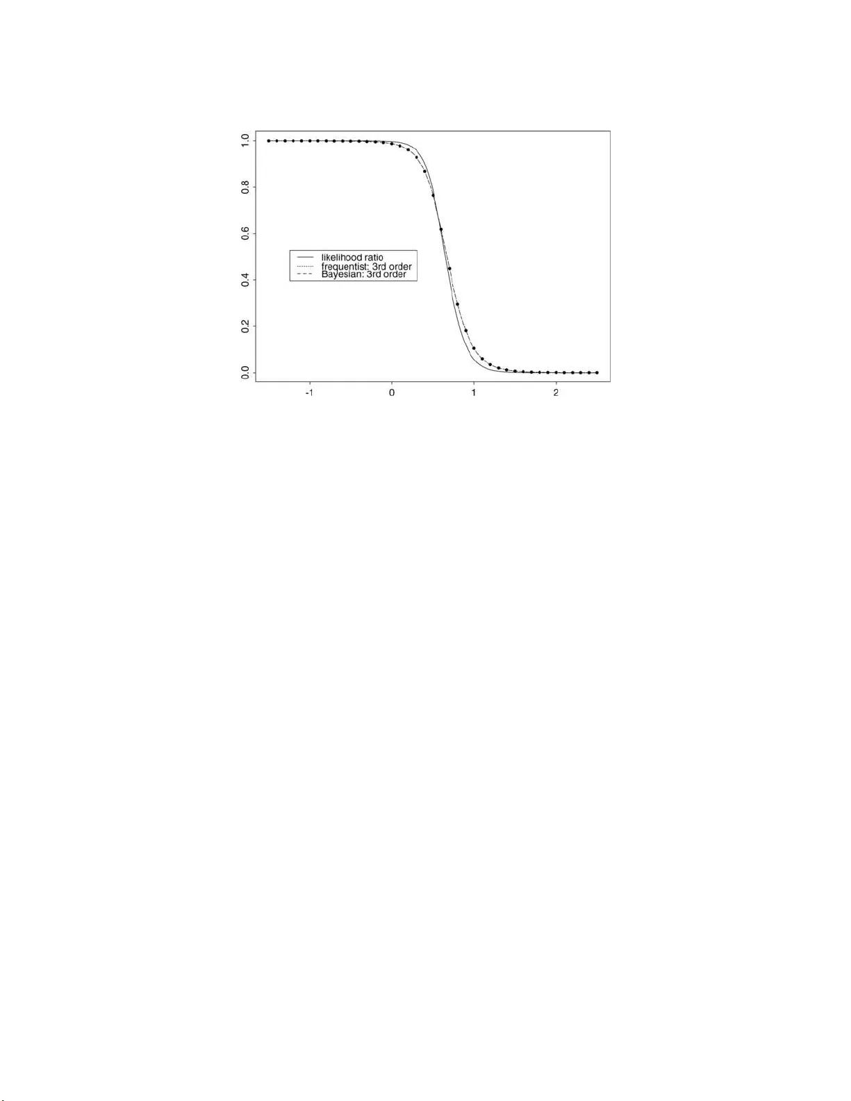
Statistic al Scienc e 2007, V ol. 22, No. 3, 301– 321 DOI: 10.1214 /07-STS240 c  Institute of Mathematical Statisti cs , 2007 Higher Accuracy fo r Ba y esian and F requentist Inference: La rge Sample Theo ry fo r Small Sample Lik eliho o d M. B´ eda rd, D. A. S. Fraser and A. W ong Abstr act. Recen t lik eliho o d theory pro du ces p -v alues that ha ve remark able accuracy and wide applicabilit y . The calculations use familiar to ols suc h as maxim u m lik eliho o d v alues (MLEs), observ ed information and p arameter rescaling. The usu al ev aluation of suc h p -v alues is by sim ulations, and suc h simulat ions do verify th at the global dis- tribution of the p -v alues is uniform(0, 1), to high accuracy in rep eated sampling. The deriv ation of the p -v alues, how eve r, asserts a stronger statemen t, that they ha v e a un i- form(0, 1) distrib ution conditionally , giv en id en tified precision inform ation pro vided b y the data. W e tak e a simple regression example that in v olv es exact precision infor- mation and use large sample tec hniqu es to extract h ighly accurate information as to the statistical p osition of the data p oin t with resp ect to the parameter: sp ecifically , w e examine v arious p -v alues and Ba ye sian p osterior survivo r s -v alues for v alidit y . With observ ed data we n umerically ev aluate the v arious p -v alues and s -v alues, and w e also record the related general formulas. W e then assess the n umerical v alues for accuracy using Mark o v c h ain Mon te Carlo (McMC) metho ds. W e also prop ose some third-order lik eliho o d-based pro cedur es f or obtaining means and v ariances of Ba y esian p osterior distributions, again follo wed by McMC assessment. Finally we pr op ose some adap- tiv e McMC metho ds to impr o v e the sim ulation acceptance rates. All these metho ds are based on asymptotic analysis that deriv es from the effect of additional data. An d the metho ds use simple calculations based on familiar m aximizing v alues and related informations. The example illustrates the general formulas and the ease of calc ulations, while the McMC assessments demonstr ate the numerical v alidit y of the p -v alues as p ercentag e p osition of a data p oin t. T he example, how ev er, is ve ry simp le and transparent, and th us giv es little ind ication that in a wide generalit y of mo dels the form ulas do accu- rately separate information for almost any parameter of interest, and then d o giv e accurate p -v alue determinations from that information. As illustration an enigmatic problem in the literature is discus sed an d simulat ions are recorded; v arious examp les in the literature are cited. Key wor ds and phr ases: Asymptotics, Ba y esian p osterior s -v alue, canonical parame- ter, d efault prior, higher o rd er , lik eliho o d , maxim u m likelihoo d departure, Met rop olis– Hastings algorithm, p -v alue, r egression example, third ord er. Myl ` ene B´ eda r d is A s sistant Pr ofessor, D´ ep artement de Math ´ ematiques et de Statistique, Universit´ e de Montr´ eal, C.P. 6128, suc c. Centr e-vil le, Montr´ eal, Qu´ eb e c, Canada H3C 3J7 e-mail: b e dar d@dms.umontr e al.c a . D. A. S. F r aser is Pr ofessor, Dep artment of Statistics, University of T or onto, 100 St Ge or ge St., 6th flo or, T or onto, Ont ario, Canada M5S 3G3 e-mail: dfr aser@u tstat.tor onto.e du . A. Wong is Pr ofessor, Dep artment of Mathematics and Statistics, Y ork U niversity, 4700 Ke ele Str e et, T or onto, Ont ario, Canada M3J 1P3 e-mail: august@yorku.c a . This is an electronic repr int of the origina l article published b y the Institute of Mathematical Statistics in Statistic al S cienc e , 2007, V o l. 22, No. 3, 301 –321 . This reprint differs fr om the or iginal in pagination a nd t yp ogr aphic detail. 1 2 M. B ´ EDARD, D. A . S. FRASER AND A. WONG 1. INTRODUCTION W e explore v arious large samp le and lik eliho o d metho ds f or obtaining Ba y esian and frequen tist p - v alues fr om a regula r statistica l mo del and d ata. Numerical v alues are obtained for a simple example that indicates the ease with whic h the metho ds can b e app lied, giv en the t ypically a v ailable maxim um lik eliho o d and related calc ulations. T he general for- m ulas are present ed and discussed . The example, ignoring the nonnormalit y of er- ror, is simple and transparent: one could p lot the data, calculate means and standard deviations, do the b o otstrap, or ev en record lik eliho o d an d get broadly ab out the same answer. But the large sam- ple tec hniqu es, more exactly data-accretion tec h - niques, pro vide accurate separation of comp onent parameter information, precisely summarize the a v ailable information, and giv e accurate d etermina- tions of corresp onding p -v alues. In Section 2 w e tak e a pr agmatic approac h and ob- tain p -v alues using simp le departu re measures and distributional appro x im ations related to the Cen tral Limit Theorem. Then in Section 3 we formally refer- ence the statistic al mo del and obtain a p -v alue based on the signed lik eliho o d ro ot. In Section 4 w e add a widely accepted default prior and obtain the p os- terior survivor v alue, the analogue of the frequen- tist p -v alue. F or the example these requir e three- dimensional inte gration. But then in Section 5 we examine recen tly de- v elop ed likel iho o d-based appro ximations that h a v e third-order accuracy; n umerical v alues are obtained for the example, and the general formulas are dis- cussed. In S ection 6 we d iscu ss the corr esp onding frequent ist third-order p -v alues. Nu merical v alues for th e example are then present ed toge ther with v arious in termediate v alues that ind icate how the calculatio ns p ro ceed. In Sect ions 7 and 8 w e consid er exac t p -v alues for the preceding methods, as deriv ed by Mark o v chain Mon te Carlo. As part of th is w e note that a N = 4 × 10 6 sim ulation in the particular co nte xt giv es ab out t wo- figure accuracy for probabilities, ab out the same as the th ir d-order appro ximation method s. In Section 9 w e briefly discuss the role of precision information in the Ba y esian and frequen tist con- texts. Section 10 lo oks directly at Ba ye sian means and v ariances and how th ey can b e approxima ted b y recen t lik eliho o d-based metho ds. Again Marko v c h ain Mon te Carlo is u sed to ev aluate the ac curacy . Section 11 pr esen ts s ome in tuitive thoughts on the Metrop olis–Hastings s tep in Marko v c hain Mon te Carlo and th en prop oses seve ral asymptotic and adaptiv e mod ifications of the direct McMC approac h; these are e xplored f or p -v alues i n S ections 12 and 13 . A con tro ve rsial example is examined in Section 14 , and some concluding remarks are recorded in a dis- cussion Section 15 . The Ba y esian and f requent ist m etho ds give ab out the same answer for the example. In fact, for the par- ticular example th ey giv e theoretica lly the same an- sw er, a consequence o f the j u dicious c h oice of d efault prior for the Ba y esian an alysis. W e do not add ress here the m anner of making such judicious choic es or h o w the c hoice t ypically n eeds to b e targeted on the particular parameter of int erest; this will b e ad- dressed sub s equen tly . 2. A S IM PLE EXAM P LE: DEP ARTURE OF D A T A FROM P ARAMETER V ALUE Consider an example to illustrate the formulas coming from large sample or, more exactly , data- accretion tec hniques: a small data set in v olving a resp onse y with p ossible linear dep end ence on a re- lated v ariable x : x − 3 − 2 − 1 0 1 2 3 y − 2.68 − 4.02 − 2.91 0.22 0.38 − 0.28 0.03 (1) The resp onse v ariabilit y is tak en to be thic ker tailed than the normal, sa y the frequent ly suggested Stu- den t(7) d istribution. Then with linear dep endence and constan t respons e v ariabilit y , w e ha ve the mo del f ( y ; θ ) = σ − 7 7 Y i =1 h { σ − 1 ( y i − α − β x i ) } , where h ( z ) = { Γ(4) / Γ(1 / 2) Γ(7 / 2) √ 7 } (1 + z 2 / 7) − 4 is the Studen t(7) density . O r using qu an tile func- tion form, w e can write y i = α + β x i + σ z i , where the laten t errors z i are indep en den t Studen t(7). No w supp ose we are interested in assessing the r esp onse dep end ence on x as given by the regression param- eter β , with particular interest in whether β = 1. As bac kground w e n ote that the resp onse data w ere in fact generated from the giv en mo del with Student(7 ) error and then rounded to tw o d ecimal places; the parameter v alues u sed to generate the data were α = 0, β = 1 and σ = 1 . I n passing we note that σ is an error scaling and do es not r ecord directly the error standard deviation. Also there is no implied connection b etw een the num b er of ob- serv ations n = 7 and the degrees of freedom f or the HIGHER AC CURACY F OR BA YESIAN AND FREQUENTIST INFERENCE 3 error density d f = 7. The example h as simple and transparent stru cture, and w e use it to examine v ar- ious frequ en tist and Ba yesian assessmen t metho ds; w e then app ly Mark o v chai n Mon te C arlo sampling to chec k the d istributional v alidit y of the r esulting v alues. The example is simple and transparent and we could probably do as w ell by plotting or by least squares and standard deviations. The lik eliho o d mo del theory , h o w ev er, giv es a precise sep aration of information concerning p arameters of in terest and an ac curate determination of the p -v alue or p ercent- age p osition of d ata with resp ect to a v alue for the parameter of interest. As a more general illustra- tion, w e later record simula tion data for a c halleng- ing e xample from the literature. W e also cite v arious examples that ha v e b een examined in the literature. F or the example considered, a pr agmatic first step is to u se least squares to separate out the general lo cation and the linear dep end en ce on the r elated v ariable x . T h e fitted v alues for α and β are a = − 1 . 322857 , b = 0 . 6750 00 , with residu al length s = (SSR) 1 / 2 = 2 . 660046 ob- tained fr om the sum of squares of residu als. The parameter β records the indicated linear d e- p end en ce of y on x . T o assess th e v alue β = 1 in the presence of the d ata, we can reasonably exam- ine the raw dep arture b − β = − 0 . 3250 00, and then standardize it by its estimat ed sta nd ard deviation to obtain a standardized measure of departure of data from parameter v alue, giving t = b ( y ) − β s/ √ 5 √ 28 , (2) t 0 = 0 . 6750 00 − 1 2 . 6600 46 / √ 5 √ 28 = − 1 . 4456 34 . T o in terpret this statistica lly w e need inf orm ation concerning the distrib ution of p ossible v alues for t in the con text wh ere th e true v alue of β is 1. T o this end , some reference to large sample theory sug- gests th e use of the standard normal distribution function, sa y Φ( · ). T he obs erv ed v alue of this dis- tribution fu nction then giv es an approximat ion to the p ercenta ge of p ossible v alues of t that w ould b e less than the obser ved t 0 , in other w ords, to the p ercenta ge p osition of th e data with resp ect to the h yp othesized v alue β = 1; this is call ed the observ ed p -v alue. Usin g the stand ard normal then as an ap- pro ximation, we obtain the approximat e p -v alue p N = Φ ( t 0 ) = Φ( − 1 . 445634) (3) = 0 . 07414 = 7 . 41 4% , whic h records the observed lev el of significance in an elemen tal form, as just th e p ercen tage p osition of the d ata p oin t or the p robabilit y left of the data p oint, under the hyp othesis. A simp le mo d ification h op efully to accommo date the estimation of error scaling is obtained by using the Student(5 ) distribution function, sa y H 5 ( · ), as a revised appr oximati on metho d . W e then obtain the appro ximate p -v alue p S = H 5 ( t 0 ) = H 5 ( − 1 . 4456 34) (4) = 0 . 10395 = 10 . 3 95% . An alternativ e to th e direct u se of th e large sample distribution theory is pro vided b y the b o otstrap ap- proac h. Using the least squares v alues, we separate the data v alues into a lo cation or fit comp onent ˆ y i and a resid u al comp onent y i − ˆ y i : x − 3 − 2 − 1 0 1 2 3 ˆ y − 3.3479 − 2.6729 − 1.9979 − 1.3229 − 0. 6479 0.0271 0.7021 y − ˆ y 0.6679 − 1.3471 − 0.9121 1.5429 1.0279 − 0.3071 − 0.6721 F or the b o otstrap w e randomly sample the r esiduals with equal p robabilit y and add them bac k to the lo- cation comp onent, th us obtaining a b o otstrap data set, from whic h w e calculate the b o otstrap t -statistic v alue t ∗ = b ∗ − 1 s ∗ / √ 5 √ 28 , where b ∗ and s ∗ are the regression co efficien t and residual length fr om the b o otstrap samp le. W e re- p eated this b o otstrap sampling a con v enien t total of N = 10 , 0 00 times, and the empirical d istribu- tion fun ction was ev aluated at the observed t 0 = − 1 . 4456 34. This ga v e an obs erv ed b o otstrap p -v alue: p BS = ˆ F ( t 0 ) = 0 . 1051 = 10 . 51% , (5) where ˆ F ( t ) is the empirical distribution f unction of the b o otstrap t ∗ v alues. With th e present small sample size n = 7 we can calculate the b o otstrap p -v alue exactly , p ExBS , by using equal pr obabilit y for eac h of the 7 7 = 823 , 543 p ossible b o otstrap samp les. W e th en tak e p ExBS = { prop ortion( t ∗ < t 0 ) (6) + pr op ortion( t ∗ ≤ t 0 ) } / 2 , 4 M. B ´ EDARD, D. A . S. FRASER AND A. WONG T able 1 Simple fr e quentist p -values for the r e gr ession example i n Se ction 2 Measure of departure Distributional approxima tion p -v alue β = 1 β = 1 . 5 β = 2 t -statistic Normal 0.07414 0 . 0 3 121 0 . 0 8 189 t -statistic Student(5) 0.10395 0 . 0 2 722 0 . 0 2 100 t -statistic Bootstrap N = 10 4 0.10750 0 . 0 2 790 0 . 0 3 800 t -statistic Bootstrap (exact) N = 7 7 0.10332 0 . 0 2 833 0 . 0 3 888 SLR Normal 0.05774 0 . 0 2 148 0 . 0 4 830 A p -va lue records the p ercentage p osition of the data relative to a p ossible t ru e v alue β for the p arameter; β = 1 is in fact the true v alue underlying the data set; β = 1 . 5 and β = 2 are other v alues that might hav e b een of in terest. Multiple zeros are indicated by a superscript, thus 0 . 0 2 148 = 0 . 00148 . called a m id - p -v alue, and obtain p ExBS = 0 . 10332 31 = 10 . 332%; (7) with our particular round ed t 0 v alue there were no v alues at the b ou n dary p oin t. T hese f our approx- imate p -v alues make use of a pragmatic c hoice of departure measure com bined with distributional in - formation pro vided by Cent ral Limit Theorem-t yp e appro ximations or b y resampling from the nonpara- metric maximum lik eliho o d distrib ution; and they pro vide us with four determinations of the observ ed p ercenta ge p osition of the data relat iv e to the mod el with β = 1. Other initial d eparture m easures could ha v e b een considered, as w ell as other distributional appro ximations or determinations. These p -v alues for testing β = 1 are recorded in T able 1 together with a lik eliho o d-based metho d dis- cussed in the next section. The table also records p -v alues for testing the more extreme β v alues, 1 . 5 and 2, with corresp ondin g observe d v alues t 0 = − 3 . 6696 85 and t 0 = − 5 . 893737. 3. THE EXAMPL E: SIMP LE LIKELIHOOD DEP A RTURE MEASURE More in trinsic dep artu re measures are a v ailable from long a v ailable lik eliho o d theory . The lik eliho o d function in the p resen t Student regression con text is L ( α, β , σ ; y ) (8) = cσ − 7 7 Y i =1  1 + ( y i − α − β x i ) 2 7 σ 2  − 4 , with log-lik eliho o d ℓ ( α, β , σ ; y ) = a − 7 log σ (9) − 4 7 X i =1 log  1 + ( y i − α − β x i ) 2 7 σ 2  ; the observ ed likel iho o d L 0 ( α, β , σ ) and observe d log- lik eliho o d ℓ 0 ( α, β , σ ) are obtained b y sub stituting the d ata y 0 = ( y 0 1 , . . . , y 0 7 ) from th e d ata arr a y ( 1 ) in to the ab ov e exp ressions. In a ge neral conte xt the observed likeli ho o d fu nc- tion is given as L 0 ( θ ) = L ( θ ; y 0 ) = cf ( y 0 ; θ ) = f 0 ( θ ) , whic h is the observed den sit y function, th at is, the statistica l mo del f ( y ; θ ) examined at the observ ed data p oin t y 0 ; it records the amoun t of p robabilit y sitting at that d ata p oin t, viewed as a function of p ossible v alues for the parameter. The co nstant c is tak en as arbitrary but p ositiv e and in dicates that only relativ e v alues from one θ v alue to another are of relev ance give n the data p oint . If w e consider in general ho w lik eliho o d dep ends on data w e can write L ( θ ; y ) = cf ( y ; θ ) , ℓ ( θ ; y ) = a + log f ( y ; θ ) , where c > 0 and a, c are otherwise arbitrary for eac h c h oice of data p oint y . Supp ose no w that we are in terested in a scalar comp onent ψ = ψ ( θ ). Most lik eliho o d m etho ds mak e use of maxim um lik eliho o d v alues (MLEs); w e do, ho w ev er, av oid r eferring to them as estimates, as they are useful but t ypically n ot dir ectly as esti- mates. W e write ˆ θ = arg sup L ( θ ) f or the v alue th at maximizes L ( θ ). Also if ψ ( θ ) is a comp onen t parameter of particular interest, we write ˆ θ ψ = arg sup ψ ( θ )= ψ L ( θ ) for th e v alue that maximizes L ( θ ) sub j ect to the in terest p arameter ψ ( θ ) h a ving some v alue ψ ( θ ) = ψ of sp ecial in terest. T hen b ased on the lik eliho o d L ( θ ) alone, an imp ortan t departure measure of data from ψ ( θ ) = ψ is obtained as the signed lik eliho o d ro ot (SLR) r ψ = sign( ˆ ψ − ψ )[2 { ℓ ( ˆ θ ) − ℓ ( ˆ θ ψ ) } ] 1 / 2 ; (10) this measur e examines ho w probability at th e data p oint u nder the full mo d el exceeds that when ψ ( θ ) is restricted to the v alue ψ , and th eory has sho wn it to b e fundamen tal. One w ay of viewin g this mea- sure is to p icture how muc h the log-lik eliho o d rises from the maxim um w h en ψ ( θ ) = ψ up to the o ve r- all maxim um when θ is u nrestricted, that is, ℓ ( ˆ θ ) − HIGHER AC CURACY F OR BA YESIAN AND FREQUENTIST INFERENCE 5 Fig. 1. F or the example in Se ction 2 : the thir d-or der Bayesian survivor function, the thir d-or der fr e quentist p -value and the first-or der SLR p -value. ℓ ( ˆ θ ψ ), often w ritten ˆ ℓ − ˜ ℓ . W e tak e th is rise as ha v- ing quadratic form r 2 ψ / 2 in terms of s ome qu an tit y r ψ ; solve for r ψ ; and then attac h the appr opriate sign. F or testing a true v alue ψ ( θ ) = ψ the signed lik eliho o d r o ot r ψ has to first order a standard nor- mal limiting distribution, a follo w -through from the Cen tral Limit Theorem. Related measur es could b e based on the slop e of the log-lik eliho o d at th e tested v alue or on the displacemen t from ˆ θ ψ to ˆ θ , but n ei- ther has the same mathematical inv ariance or th e same trac k record in applications. F or m an y likeli ho o d calculations, particularly re- cen t h igher-order calculatio ns, the computationally c h allenging asp ects often arise in the maximization steps rather th an in other steps. F or our simple regression example and the related lik eliho o d calculations we no w use maximum like - liho o d rather than least squares v ariables; the ob- serv ed v alues obtained b y compu ter iteration are ˆ α = − 1 . 350451 2 , ˆ β = 0 . 65040 19 , ˆ σ = 0 . 9641 110 for the o v erall MLE s , and ˜ α = ˆ α β =1 = − 1 . 366699 , ˜ β = ˆ β β =1 = 1 , ˜ σ = ˆ σ β =1 = 1 . 154 527 for the constrained MLEs w hen β = 1. In passin g w e note that th e u se of MLE v ariables can b e con- v enien t but can b e awkw ard when the error distri- bution i tself has dep endence on the parameter; for if the distrib u tion for the error itself has dep endence on the parameter r ather than as here b eing just S tu- den t(7), then the maximum lik eliho o d v alue could also hav e that parameter dep end ence and th us not b e a statistic. F rom the p receding n umerical v alues w e obtain from ( 10 ) the signed likel iho o d r o ot r β =1 = − 1 . 574053 . (11) The co rresp onding observ ed p -v alue based on the first-order normal approxima tion for r is then p SLR = Φ( r β =1 ) = 5 . 774%; (12) this is also recorded in T able 1 . In Figure 1 we plot the SLR p -v alue against a full range of p os- sible β v alues; this is called the p -v alue function; some related determinations d iscussed in later sec- tions are also recorded in the figure. Other lik eliho o d departure measures based on the score and maxi- m um lik eliho o d estimates are sometimes considered, but they frequentl y hav e serious distribu tional and measuremen t bias d iffi cu lties. By con trast, the SLR- based appro ximate p -v alue u s es a departure mea- sure that directly relates to the statistical mo del; it summarizes bac kground information con tained in the mo d el com bined with distr ib utional information deriv ed from the large sample b eha vior of the lik e- liho o d function. 6 M. B ´ EDARD, D. A . S. FRASER AND A. WONG 4. ANAL YSIS WITH DEF A UL T PRIOR An alternativ e first-order likel iho o d-based metho d comes from the use of a mod el-based flat prior called a d efault prior together with co nditional-probabilit y t yp e calculations, t ypically referr ed to as Bay es al- gorithm. L et π ( θ ) b e a w eigh t fun ction for θ based on symmetries, inv ariance, or other relev ant prop er- ties of the mo del. The corresp ond ing p osterior dis- tribution viewe d as pro viding in f erence inform ation concerning θ is π ( θ | y 0 ) = cπ ( θ ) L ( θ ) , (13) where c no w indicates the normin g constant . T his default appr oac h w as implicit in Ba yes ( 1763 ), was strongly p romoted by Laplace ( 1812 ) and Jeffreys ( 1946 ) and ac quired th e n ame inv erse p robabilit y . More recen tly its dev elopmen t has b een stimulated b y the V alencia conferences (see, e.g., Ba yesia n Statis- tics 7, 2003 ); the default p r iors are called ob jecti ve priors but in suc h con texts the ob jec tiv e can only refer to mo del stru cture, not to an y ob jec tiv e fre- quencies in the con text b eing examined. F or inference concernin g an interest parameter, sa y ψ ( θ ), one migh t then reasonably calculate the marginal p osterior densit y function π ( ψ | y 0 ) = Z π ( θ | y 0 ) dλ, where λ is a complemen ting n uisance parameter her e c h osen so th at θ is one– one equiv alen t to ( ψ , λ ) and to ha v e, say , Jacobian | ∂ θ/∂ ψ ∂ λ | ≡ 1 so that su p- p ort volume corrections can b e ignored. This m arginalizati on to obtain an inference dis- tribution for a comp onent parameter can pr o duce misleading results (e.g., Da w id, Stone and Z idek, 1973 ). T o o v ercome this issue, a preferr ed approac h is to ha ve a prior that d ep ends on the p articular parameter of in terest, and thus to use a targeted prior π ψ ( θ ) where the subscript ind icates the partic- ular parameter b eing targeted (e.g., Jeffreys, 1946 ; Bernardo, 1979 ; F raser et al., 2003 ). W e do not ad- dress this imp ortan t issue of c ho osing default p riors but do ac knowledge that it is of ma jor in terest f or the Ba ye sian comm unity at the p resen t time and in part for th e frequentist comm unit y . F or our sim p le regression example we might p os- sibly consid er the mo d el-based default prior π ( θ ) to b e the in v arian t pr ior π ( θ ) dθ = dα dβ dσ σ 3 = dα dβ d log σ σ 2 ; this d eriv es f rom p arameter transform ations on the sample and parameter sp aces and is referred to as the left in v ariant prior (e.g., Jeffreys, 1946 ; F raser, 1979 ): un der transform ations th at mak e lo cation and scale changes on the initial sample s pace, the dif- feren tial rewritten as, sa y , dα dβ dσ /σ 3 remains unc hanged, is inv arian t. T his left p rior av oids the marginalizatio n issues for certain p arameter com- p onents that are linear in a lo cation p arameteriza- tion implied by asymp totic theo ry (F raser and Reid, 2002 ); for many familiar parameters of interest, how- ev er, it can lead to the marginalization issues; an d furthermore it do es not corresp ond to the confid ence theory pivo tal in version based on the usual equa- tions ( y i − α − β x i ) /σ = z i . F or the parameter β , v arious approac hes (e.g., Da wid , S tone and Zidek, 1973 ; F raser, 1979 ) sug- gest the targeted pr ior π β ( θ ) dθ = dα dβ dσ σ = dα dβ d log σ, and for m any p arameters having a certain linearit y it does a vo id the ma rginalization issu e; some discus- sion of this linearit y and a r elated curv ature measure ma y b e found in F raser and Reid ( 2002 ); the curv a- ture iss ue do es not arise in the present problem for the nice paramete rs α, β , σ and w e do not pursu e the issue here. F rom the transform ation viewp oint this is called the righ t in v ariant prior. Th e c orresp onding mo del-based p osterior for θ is then giv en b y π ( α, β , τ ; y 0 ) dθ = cσ − 7 (14) · 7 Y i =1  1 + ( y 0 i − α − β x i ) 2 7 σ 2  − 4 dα dβ d log σ ; for this, if w e now tak e θ to b e ( α, β , τ ) = ( α, β , log σ ), the implied prior is π ( θ ) = 1 and it conforms to con- fidence inv ersion. In order then to obtain the marginal densit y for the in terest parameter β , an in tegration o ver α and τ is requ ired. Rep eated numerical inte gration o ve r t w o dimensions can b e quite feasible but ofte n is not easily implemente d; w e next consider some alterna- tiv e integrati on pr o cedures. F or more general use of this Ba y esian approac h the choic e of the default p rior b ecomes a crucial is- sue and is the fo cus of m uch present activit y in the Ba yesia n comm u nit y; the term ob ject ive Ba ye sian prior is sometimes used in place of the term default HIGHER AC CURACY F OR BA YESIAN AND FREQUENTIST INFERENCE 7 Ba yesia n prior, bu t this is misleading as the ob jec- tiv e w ould indicate that it is describin g the ph ysical con text rather than b eing based as here on mo del c h aracteristics, a leve l remo v ed f rom the physical con text. 5. THIRD ORDER WITH DEF AU L T PRIOR F or man y regular densities, p osterior or otherwise, the L ap lace in tegration m etho d provi des an accu- rate alternativ e route f or obtaining the marginal densit y of a comp onen t, suc h as β in our case. As b efore, bu t in general notation, w e use π ( ψ , λ ) for the p rop osed prior and L ( ψ, λ ) f or the like liho o d . Then with third-ord er accuracy , the marginal p os- terior density for ψ can b e obtained by Laplace in- tegration o ver the n u isance parameter divided b y Laplace in tegration o v er the f ull parameter, giving π ( ψ ; y 0 ) = e k /n (2 π ) d/ 2 (15) · e − r 2 ψ / 2  | ˆ j θ θ | | j λλ ( ˆ θ ψ ) |  1 / 2 π ( ˆ θ ψ ) π ( ˆ θ ) , where k indicates a firs t-order constan t: r 2 ψ is th e lik eliho o d ratio quantit y r 2 ψ = 2 { ℓ ( ˆ θ ) − ℓ ( ˆ θ ψ ) } (16) discussed earlier but no w used more generally w ith ψ of dimension d , nuisance parameter λ of dimension m , and p = d + m ; the Hessian matrices j θ θ ( θ ; y ) = − ∂ 2 ∂ θ ∂ θ ′ ℓ ( θ ; y ) , j λλ ( θ ; y ) = − ∂ 2 ∂ λ ∂ λ ′ ℓ ( θ ; y ) are information functions for the full and f or the n uisance parameters, a nd ha v e dimensions p × p and m × m ; they are just negativ e second-deriv ativ e ma- trices of the log-lik eliho o d fun ction, and when ev al- uated at ˆ θ and ˆ θ ψ giv e the observed information matrices ˆ j θ θ = j θ θ ( ˆ θ ; y ) , (17) ˜ j λλ = j λλ ( ˆ θ ψ ) = j λλ ( ˆ θ ψ ; y ) . Numerically , the information matrices can t ypically b e computed b y taking second differences based on v ery small an d equ ally sp aced v alues for eac h co or- dinate. The preceding m arginal density can also b e w rit- ten π ( ψ ; y 0 ) = e k /n (2 π ) d/ 2 L P ( ψ ) L P ( ˆ ψ ) (18) ·  | ˆ j θ θ | | j λλ ( ˆ θ ψ ) |  1 / 2 π ( ˆ θ ψ ) π ( ˆ θ ) , where L P ( ψ ) = sup λ L ( ψ , λ ) = L ( ψ , ˆ λ ψ ) is the pr ofile lik eliho o d fu nction for ψ , obtained by maximizing the fu ll lik eliho o d o v er λ for fixed v alue ψ of the int erest parameter ψ ( θ ) . The m etho ds inherent in th e Laplace integrat ion pro cedur e can b e describ ed fairly easily . A regular function, here L ( ψ , λ ) for fixed ψ , wh ose logarithm has additiv e and m axim um lik eliho o d v alue prop er- ties u nder incr easing sample size n can b e rewritten f ( λ ) = e h ( λ ) = c exp {− ˆ j λλ λ 2 / 2 } exp { aλ 3 / 6 n 1 / 2 + bλ 4 / 24 n } to th ird order as a fu nction of λ , with ob vious gen- eralizatio n for vec tor λ ; for this we are letting λ designate a stand ardized departu re of th e original λ fr om the maximizing v alue for f ( λ ) with ψ fixed. After expanding the second exp onential in a p o w er series and similarly for the log-prior, and then inte- grating term b y term with resp ect to λ , w e obtain to fourth ord er, Z f ( λ ) π ( ψ , λ ) dλ = e k /n (2 π ) m/ 2 | ˆ j λλ ( ψ ) | − 1 / 2 f ( ˆ λ ψ ) π ( ψ , ˆ λ ψ ) , where ˆ j is the n egativ e Hessian with resp ect to λ as ev aluated at the maximum f or the fi xed ψ . The in- tegrations a re based on simple reference to the mul- tiv ariate normal integ ral; for some bac kground, see Stra wderman ( 2000 ) and for some discussion of term b y term integrati on, see Andrews, F raser and W ong ( 2005 ). F or a scalar in terest parameter ψ w e can reason- ably b e more interested in an in tegral of its den- sit y fun ction, an d p articularly in th e r ight tail in- tegral called the p osterior sur viv or function. Wh y the right tail? C onsider th e simple case of a v ari- able x measuring a parameter ψ with err or densit y f ( e ) and distrib ution function F ( e ); we h a v e: the observ ed p -v alue is p 0 ( ψ ) = F 0 ( ψ ) = F ( x 0 − ψ ); the 8 M. B ´ EDARD, D. A . S. FRASER AND A. WONG righ t tail p osterior sur viv or function with a natu- ral fl at pr ior is s ( ψ ) = R ∞ ψ f ( x 0 ; α ) dα = R ∞ ψ f ( x 0 − α ) dα = F ( x 0 − ψ ); and these are equal. In m ore general mo del situations the p -v alue as discussed in the n ext section records in a statistical sense where the data v alue is with resp ect to ψ in a left-to-righ t distributional s en se and then corresp onds as in the simple case to the su rviv or p osterior v alue s ( ψ ) . F or the general case a highly accurate appr o xima- tion to the p osterior surviv or fun ction is a v ailable from lik eliho o d theory (see, e.g., F raser, Reid and W u , 1999 , generalizing DiCiccio and Martin, 1991 ): s ( ψ ) = 1 − G ( ψ | y 0 ) (19) = Φ  r − r − 1 log r q  = Φ( r ∗ ) . F or this, G designates the p osterior d istribution fu nc- tion for ψ , r is the signed lik eliho o d r o ot r ψ giv en as ( 10 ) in S ection 3 , q B is a score-t yp e departure measure for ψ , q B = ℓ ψ ( ˆ θ ψ )  | ˆ j λλ ( ˆ θ ψ ) | | ˆ j θ θ |  1 / 2 π ( ˆ θ ) π ( ˆ θ ψ ) , (20) where ℓ ψ ( θ ) = ∂ ∂ ψ ℓ ( ˆ θ ψ ) = ∂ ∂ ψ ℓ ( θ ; y 0 )    ˆ θ ψ (21) is a score departure measur e, and r ∗ is implicitly defined. Note that for conv enience w e ha v e tak en the full p arameter θ to b e give n as ( ψ , λ ′ ) ′ in terms of the comp onents, and this applies as w ell to the information matrices at ( 17 ). Also we h a v e c hosen to record the u pp er tail for present ing p osterior probability from the p osterior distribution; the interest parameter will often ha v e physic al meanin g in a p articular applica tion and in- v estigators will think in terms of a v ariable mea- suring the parameter as, sa y , with a maximum lik e- liho o d estimate. In such a framew ork th e us ual p - v alue is left tail for the v ariable and corresp ond ingly is right tail for the parameter as in the location case; accordingly for harmony b et w een the t w o inference approac hes w e tak e the reference Ba y esian probabil- it y to b e the up p er tail s urvivo r v alue. In th e n ext section w e will find that formula ( 20 ) using r from ( 10 ) and q B from ( 20 ) can b e derived directly from frequent ist formulas in the n ext section by acting as if π ( ψ ; y 0 ) in ( 15 ) w ere obtained f rom a lo cation mo del π ( ψ − x ; y 0 ) with a nominal v ariable x taking the observe d v alue x = 0. F or our simple example and testing β = 1, w e h a ve r = − 1 . 57405 3 from ( 11 ) and w e ha v e q B = − 0 . 948368 6 , (22) where ℓ β ( ˆ θ β =1 ) = − 5 . 8686 99 , and the full and constrained information matrices for θ = ( α, β , τ ) are ˆ j θ θ = j θ θ ( ˆ θ ) (23) = 911 5 . 78941 95 1 . 31106 0 − 0 . 328683 7 1 . 31106 0 27 . 28 8552 − 1 . 3395559 − 0 . 328683 7 − 1 . 339556 12 . 1900 132 ! , j λλ ( ˆ θ β ) = 911  4 . 02406 89 − 0 . 33195 37 − 0 . 331953 7 8 . 59256 87  , (24) with corresp onding determinant s | ˆ j θ θ | = 1892 . 7 02 , (25) | j λλ ( ˆ θ β ) | = 34 . 46 69 . This giv es r ∗ = − 1 . 25 2169; the Ba y esian p osterior survivo r v alue fr om (18) is then s B (1) = 0 . 1052 542; (26) this is recorded in T able 2 together with the Ba ye sian survivo r v alues for testing β = 1 . 5 and β = 2, as w ell as some McMC v alidation results discussed in later sections. The first-order lik eliho o d metho d in Section 3 re- quires the full and the constrained maximum lik e- liho o d v alues ˆ θ and ˆ θ ψ with of course corresp ond- ing v alues for the log-lik eliho o d fun ction. In ord er to tak e adv ant age of th e app ro ximate int egration form ulas in this section, we require in addition the second-deriv ativ e v alues at eac h MLE; such deriv a- tiv es are of course also needed for f amiliar score and MLE departure m easures and t ypically can b e ob- tained by differencing. W e can also calculate the Ba ye sian su rviv or v alue s ( β ) for a range of v alues for β . F or our sp ecial ex- ample the Ba y esian survivor function s B ( β ) is plot- ted in Figure 1 together with the lik eliho o d ratio p -v alue Φ( r β ) and a third -order fr equen tist p -v alue to b e discussed in the next section. HIGHER AC CURACY F OR BA YESIAN AND FREQUENTIST INFERENCE 9 6. THIRD-ORDER p -V ALUE Recen t lik eliho o d metho ds giv e h ighly accurate appro ximations f or frequen tist inference in muc h th e same manner as for the Ba y esian con text just de- scrib ed. Th e metho ds require fu ll and constrained maxim um lik eliho o d v alues ˆ θ and ˆ θ ψ , as we ll as full and constrained information determinan ts. They also, ho w ev er, n eed something more in the wa y of information f r om th e mo del and data. T he nature of this extra information can b est b e describ ed in terms of parameterizatio n scaling or reexpression. In particular, we need to express the initial parame- ter θ as a canonical-t yp e parameter, s a y ϕ = ϕ ( θ ) . In the Ba ye sian con text, s uc h additional information is closely relate d to the deve lopment of an a ppr opriate default pr ior; thus the use of a weigh ted lik eliho o d L ( θ ) π ( θ ) can partly b e interpreted in term s of s eek- ing a lo cation r eparameterizatio n β = β ( θ ) suc h t hat π ( θ ) dθ = dβ . Ba y esian parameter rew eighti ngs ha v e long b een sought in the d ev elopmen tal sequence from in v ariant (Ba y es, 1763 ; Laplace, 181 2 ) to Jeffreys ( 1946 ) to reference p riors (Bernardo, 1979 ). In the fr equen tist con text the accessible reparam- eterizatio ns are of a n expon ential rather than a lo ca- tion t yp e, bu t they giv e some access to th e related lo- cation information. The exp onential -t yp e reparam- eterizatio n can b e examined initially in the con text of an exp onenti al mo del. T o this effect, consider an exp onentia l mo del with canonical parameter ϕ , f ( y ; ϕ ) = exp { ϕ ′ s ( y ) − κ ( ϕ ) } h ( y ) , (27) where ϕ and s ha v e the same d imension, sa y p . F or s uc h a mo del, the saddlep oin t appro ximation (Daniels, 1954 ) can be r emark ably a ccurate, and has the density form ¯ f ( y ; ϕ ) dy = e k /n (2 π ) p/ 2 e − r 2 / 2 | ˆ j ϕϕ | 1 / 2 d ˆ ϕ (28) = e k /n (2 π ) p/ 2 e − r 2 / 2 | ˆ j ϕϕ | − 1 / 2 ds, (29) where r 2 is the lik eliho o d rati o qu an tit y for assessing the full paramete r ϕ and ˆ j ϕϕ = − ( ∂ 2 /∂ ϕ 2 ) ℓ ( ϕ ; y 0 ) | ˆ ϕ is the obser ved information matrix from a d ata p oin t y . The r enormalized ( 28 ) is third-order accurate. F or the imp ortan t sp ecial case of a scalar parame- ter ϕ , a corresp ondin g distrib ution fu nction appro xi- mation w as dev elop ed by Lu gannani and Rice ( 1980 ) and in an alternativ e form by Barndorff- Nielsen ( 1991 ). Both versions use the signed like li- ho o d ratio r = r ( ϕ, s ) corresp onding to ( 10 ), plus a maxim um likel iho o d v alue d ep arture q = q ( ϕ, s ): q f = ( ˆ ϕ − ϕ ) ˆ j 1 / 2 ϕϕ . The approximat e distribution function in the Barndorff-Nielsen ( 1991 ) form for ˆ ϕ or s is then ¯ F ( s ; ϕ ) = Φ  r − r − 1 log r q f  = Φ( r ∗ ) , (30) and has third-order accuracy; this has the same form as ( 19 ) but uses a different departure q appropr iate to the presen t frequentist context. The similarit y of the Ba y esian formula ( 19 ) and the ab o v e f requen- tist formula can app ear more p lausible by defining the follo w ing reexpressions of the v ariable and the parameter: β ( ϕ ) = Z ϕ ˆ j 1 / 2 ϕϕ d ˆ ϕ, b ( s ) = Z s ˆ j − 1 / 2 ϕϕ ds. T able 2 F or the simple r e gr ession example in Se ction 2 , Bayesian s -values for assessing the values β = 1 , β = 1 . 5 and β = 2 : using the thir d-or der f ormul a ( 19 ); using the McMC (Se ction 8 with Normal pr op osal); using AMcMC (Se ction 12 w i th adap tive choic e of Student pr op osal) T est pro cedure s -v alue β = 1 β = 1 . 5 β = 2 Ba yesian: third order ( N = 4 × 10 6 ) 0.10525 0 . 0 2 725 0 . 0 3 923 Ba yesian: McMC ( N = 4 × 10 6 , Normal) 0.10744 0 . 0 2 841 0 . 0 2 118 (Simulatio n SD ) (0 . 0 3 484) (0 . 0 3 186) (0 . 0 4 789) { Acceptance rate } { 41.9% } { 41.9% } { 41.9% } Ba yesian: AMcMC ( N = 4 . 10 6 , adaptive S tudent) 0.10752 0 . 0 2 836 0 . 0 2 118 (Simulatio n SD ) (0 . 0 3 332) (0 . 0 3 100) (0 . 0 4 366) { Acceptance rate } { 51.1% } { 51.1% } { 51.1% } 10 M. B ´ EDARD, D. A . S. FRASER AND A. WONG In terms of these, W elc h and P eers ( 1963 ) sho we d in effect that b has a lo cation model f ( b − β ) to second- order accuracy . T his has profound implications for p ossible second ord er agreemen t b etw een Ba y esian and frequen tist metho dologies, but W elc h and P eers ( 1963 ) presented their results in terms of the fre- quen tist approac h of obtaining confidence b ou n ds b y in tegrating lik eliho o d with respect to the Jeffreys ( 1946 ) prior i 1 / 2 ϕϕ ( ϕ ) dϕ . Th e same result with some greater generalit y can b e ob tained by T aylo r series expansion of an asymp totic mo del with scalar v ari- able and p arameter; simple reexpressions of v ariable and parameter sho w th at to second order the mo del can be written either as a lo cation or as an exp onen- tial mo del; see, f or example, C akmak et al. ( 1998 ) and An drews, F raser and W ong ( 2005 ). A somewhat similar result is av ailable w ith vecto r v ariable and parameter; see Cakmak, F raser and Reid ( 1994 ). F or the case of a lo cation mo del f ( s − β ) with a flat p rior π ( β ) = c , th e expr ession ( 20 ) f or q B sim- plifies to q B = ℓ β ( β ) ˆ j − 1 / 2 β β . As ℓ β ( β ; s ) = ( ∂ / ∂ β ) ℓ ( β ; s ) = − ( ∂ /∂ s ) ℓ ( s − β ) = − ℓ ; s ( β ; s ) fr om the lo cation prop ert y , and − ℓ β ( β ) = ℓ ; s ( β , s ) = ϕ from the exp onent ial form ( 27 ), w e ob- tain through simple alg ebra that q f = q B , whic h im- plies that the fr equ en tist distribution function is equal to the Ba y esian survivo r function, as would b e exp ected. I n other wo rds , this W elc h and P eers ( 1963 ) Ba ye sian–frequentist equalit y is obtained from the Jeffreys prior for the scalar exp onenti al mo del, and thus as demonstrated by Cakmak et al. ( 1994 , 1998 ) has an extension for general asymptotic mod - els. The adv an tages of this scalar parameter use of the Jeffreys prior has recentl y b een d iscussed for the discrete binomial distribu tion con text by Brown, Cai and DasGupta ( 2001 ). No w consider the vecto r exp on ential mo del ( 27 ) with p -dimensional canonica l parameter ϕ and p - dimensional canonical v ariable s , and sup p ose that w e are interested in a scalar comp onent parameter ψ ( ϕ ) having reasonable smo othness prop erties. The signed lik eliho o d ro ot r = r ψ in ( 10 ) is the pri- mary departur e measure and a maxim um like liho o d departure q f ( ψ ) = sign( ˆ ψ − ψ ) (31) · | ˆ χ − ˆ χ ψ |  | ˆ j ϕϕ | | j ( λλ ) ( ˆ θ ψ ) |  1 / 2 is the secondary departure measure. F or this, θ = ( λ, ψ ) has b een presen ted as a com bination of ψ with a nuisance parameter λ whic h complements the in- terest parameter ψ ; in the v ector case we sh ould p erhap s wr ite the com bination in term of row v ec- tors as θ ′ = ( ψ ′ , λ ′ ). The scalar parameter χ ( θ ) is a rotated co ordin ate of ϕ ( θ ) that acts as a sur rogate for ψ ( θ ) and has linearit y in terms of ϕ ( θ ). Explicit form ulas f or the surr ogate parameter χ ( θ ) and the n uisance information are r ecorded in the App end ix ; some d iscussion a lso app ears in the next se ction; the paren theses around ( λλ ) are to indicate that the in- formation has b een recalibrated in terms of the new parameterizatio n ϕ . All of this is easily accessible n umerically , and u s es primarily just the typical in- gredien ts of the Ba ye sian-t yp e approximati on. 7. THIRD ORDER FOR THE EXAMPLE W e ha v e just describ ed h o w third-order p -v alues are a v ailable to assess a scalar parameter ψ ( θ ) in an exp onentia l m o del. While exponential mo d els are of course qu ite imp ortant, they do r epresen t a v ery sp e- cialize d t yp e of mo d el. How eve r, recen t likeli ho o d theory has sho wn that for a general con tin uous sta- tistical mo del together w ith data, there exists a cor- resp ond ing exp onen tial mo del that provides highly accurate third -order p -v alues f or the original mo del and data, usin g th e form ulas in the p receding sec- tion. F or our example in Section 3 , the corresp on d ing exp onentia l mod el with data h as the same obs erv ed log-lik eliho o d ℓ ( θ ) = log f ( y 0 ; θ ) giv en as ( 9 ) and has a nominal reparameterization ϕ ′ = ( ϕ 1 , ϕ 2 , ϕ 3 ) giv en as a r ow vec tor; some d iscussion is giv en later. See also Da v ison , F raser an d Reid ( 2006 ). The reparam- eterizatio n is ϕ ′ ( α, β , σ ) (32) = 8 7 X i =1 ( α + β x i − y 0 i ) / 7 σ 2 1 + ( y 0 i − α − β x i ) 2 / 7 σ 2 (1 , x i , d 0 i ) , and is explained later in d etail; here d 0 is just the standardized residual vect or ( y 0 − ˆ y 0 ) / ˆ σ 0 recorded n umerically preceding ( 35 ). The co rresp onding gen- eral form ulas are recorded at the end of this section. T o obtain the p -v alue for assessing any scalar com- p onent parameter, it suffices to treat the ob s erv ed lik eliho o d as a function of ϕ , whic h of course means explicitly or implicitly that th e observ ed inf orma- tions needs to b e reexpressed or recalibrated in terms HIGHER AC CURACY F OR BA YESIAN AND FREQUENTIST INFERENCE 11 T able 3 F r e quentist p -values for the simple r e gr ession example in Se ction 2 , for assessing t he values β = 1 , β = 1 . 5 and β = 2 : using the thir d-or der formula ( 30 ) wi th ( 11 ) and ( 31 ); using McMC with normal pr op osal c enter e d at a value at hand wi th standar d deviation 0.35 (Se ction 8 ); using McMC with a c enter e d Student(7) pr op osal; and using McMC using an adaptive Student pr op osal (Se ction 13 ) T est pro cedure p -v alue β = 1 β = 1 . 5 β = 2 F requ entist; third order 0.10525 0 . 0 2 725 0 . 0 3 923 F requ entist; McMC ( N = 4 . 10 6 , Normal) 0.1 0832 0 . 0 2 819 0 . 0 2 118 (Simulatio n SD ) (0 . 0 3 398) (0 . 0 3 109) (0 . 0 4 406) { Acceptance rate } { 38.0% } { 38.0% } { 38.0% } McMC [ N = 4 . 10 6 , Student(7)] 0.10765 0 . 0 2 827 0 . 0 2 113 (Simulatio n SD ) (0 . 0 3 196) (0 . 0 4 510) (0 . 0 4 185) { Acceptance rate } { 75.9% } { 75.9% } { 75.9% } AMcMC ( N = 4 . 10 6 , adaptive Student) 0.10792 0 . 0 2 823 0 . 0 2 109 (Simulatio n SD ) (0 . 0 3 204) (0 . 0 4 646) (0 . 0 4 264) { Acceptance rate } { 81.6% } { 81.6% } { 81.65% } of the ϕ parameterization and the maximum lik eli- ho o d departure n eeds also to b e expr essed in the ϕ parameterizatio n. The recalibration of the information is obtained from the deriv ative ϕ θ ( θ ) = ∂ ϕ/∂ α ∂ β ∂ σ of ϕ with resp ect to the initial parameters as ev aluated at the maxim um lik eliho o d v alues. F or this with ψ = β and λ ′ = ( α, log σ ) , w e ob tain ϕ θ ( ˆ θ 0 ) =   5 . 7894 195 1 . 3110 60 − 0 . 328 6837 1 . 3110 600 27 . 288 552 − 1 . 339 5559 − 0 . 328 6837 − 1 . 339 5 56 12 . 1900 132   , ϕ λ ( ˆ θ β =1 ) =   4 . 0240 689 − 0 . 33 19537 − 0 . 147 4505 − 7 . 570 6 463 − 0 . 518 8019 7 . 5500 100   . Using these as s caling matrices along with the ma- trices ( 24 ) giv es the recalibrated information deter- minan ts: | j ϕϕ | = | j θ θ || ϕ θ | − 2 = 0 . 000 528345 , | j ( λλ ) ( ˆ θ β =1 ) | = | j λλ ( ˆ θ β =1 ) || ϕ ′ λ ϕ λ | − 1 = 0 . 01844 021 . The sp ecial maxim um lik eliho o d departure used in ( 31 ) is sgn( ˆ β − β ) | ˆ χ − ˆ χ β | = − 5 . 602751 . W e then use r β =1 = − 1 . 574053 from ( 11 ) together with q β =1 = − 0 . 9483 686 (33) from ( 31 ) to substitute in ( 30 ); this give s the third- order p -v alue p 3rd = 0 . 105 25 , (34) whic h is r ecorded in T able 3 along with other v alues including those for testi ng the paramet er v alues β = 1 . 5 and β = 2. W e can also calculate the third-ord er frequentist p -v alue p ( β ) for a r ange of v alues for β ; for our ex- ample, this p -v alue function is plotted in Figure 1 using dots to allo w fo r comparison with the Ba y esian s ( β ) obtained in S ection 4 . W e record no w some general though ts on t he r ep a- rameterizatio n ϕ ( θ ). In the context w ith indep en- den t scalar co ordinates, w e h a v e ϕ ( θ ) = n X i =1 ∂ ℓ ( θ ; y i ) ∂ y i     y 0 i dy i dθ     ( y 0 i , ˆ θ 0 ) . The fi rst f actor is a f u nction of θ that records ho w the i th coord inate influ ences the likel iho o d f unction: ∂ ℓ ( θ ; y i ) ∂ y i = ∂ ∂ y i log f i ( y i ; θ ); it is the co ordinate gradien t of lik eliho o d and can b e view ed as a p arameter when the observed data v alues are substituted. F or our example w e h a v e ∂ ℓ ( θ ; y i ) ∂ y i     y 0 i = 8 ( α + β x i − y 0 i ) / 7 σ 2 1 + ( y 0 i − α − β x i ) 2 / 7 σ 2 and it app ears in ( 32 ) ab o v e. The second factor in ( 32 ) is a n umerical row v ector that records ho w pa- rameter c hange near the o v erall maximum like liho o d v alue affects the i th coordinate; it records the sensi- tivit y of th e i th co ordinate to p arameter change at the m axim um likelihoo d v alue. T his u ses the error 12 M. B ´ EDARD, D. A . S. FRASER AND A. WONG z i as an i th coordinate piv ot, whic h with co ntin uity is necessarily one–one equiv alent to the distribution function F i ( y i ; θ ); and th en with the piv ot inv erted to express y i = y i ( θ , z i ) in terms of θ and z i w e ob- tain the d eriv ativ e dy i dθ     ( y 0 i , ˆ θ 0 ) for th e i th coordin ate at the data p oin t. F or our example with z i = ( y i − α − β x i ) /σ w e obtain y i = α + β x i + σ z 0 i and then ha v e ∂ y i ∂ α = 1 , ∂ y i ∂ β = x i , ∂ y i ∂ σ = z i . Then for ev aluation at ( y 0 , ˆ θ 0 ) w e need the observ ed standardized residu al ˆ z 0 = d 0 = d ( y 0 ): d 0 = { d 1 ( y 0 ) , . . . , d 7 ( y 0 ) } ′ = (0 . 5614092 , − 1 . 1324 253 , − 0 . 7667 588 , 1 . 2969452 , 0 . 8640 297 , − 0 . 2581882 , − 0 . 5650118) ′ as calculated from d 0 i = y 0 i − ˆ α 0 − ˆ β 0 x i ˆ σ 0 . (35) W e thus obtai n the final ve ctor in (1 , x i , d 0 i ) as used in ( 32 ). F or some bac kground theory see F raser and Reid ( 1993 , 1995 , 2001 ) and for an ov erview of the metho d- ology for the r egression con text see F raser, Reid and W ong ( 2005 ), F r aser, W ong and W u ( 1999 ). 8. THE EXACT p -V ALUES AND s -V AL UES Higher-order p -v alues and higher-order p osterior survivo r s -v alues are usually v alidated by sim ula- tions, by ve rifying that the la rge sample distrib ution in eac h case is close to the un if orm (0, 1) distrib ution. The form ulas, ho wev er, h a v e b een d ev elop ed in the con text of a conditional m o del: in the Ba ye sian con- text it is cond itional on the full data, and in the fre- quen tist con text it is conditional on d ata indicators of statistical precision, whic h t ypically are given b y exact or ap p ro ximate ancillaries that reflect stru c- ture and con tinuit y of the mo del with resp ect to the v ariable and the parameter. F or a general f r equen tist context , the app r o ximate ancillaries for thir d-order inferen ce are we ll d efined theoreticall y bu t are only needed near the observ ed data p oint and t y p ically are only a v ailable n ear the observ ed data. In such con texts this can mak e a full conditional v alidation unattainable as typica lly there is no accessible in f ormation concerning other conditioned p oin ts, b eyond the tangen t direction at the data. Our example, h o w ev er, h as sp ecial lin- ear and tr ansformation prop erties that do pro vide an exact conditioning v ariable, here d ( y ) , and thus an exact conditional d istribution; some b ackg roun d and details are r ecorded in the App end ix at p oin t (i). Again as in Section 2 w e describ e the mo del in terms of the con venien t least squares co ord inates ( a, b, s ) , and then record the densit y for just the standardized or null case with α = 0 , β = 0 , σ = 1; the conditional densit y for ( a, b, s ) is g ( a, b, s ) = c 7 Y i =1 h { a + bx i + sd i } s 4 , (36) where as b efore h ( z ) is th e Stu d en t(7) density; this is derived in F r aser ( 1979 ) an d discussed briefly in F r aser ( 2004 ). Note that we could also ha ve used maxim um lik eliho o d v ariables, as the err or distribu- tion is f r ee of the parameter, but the least squares v ariables ha ve conv enien t s implicit y; the nonnull con- ditional density is then av ailable directly as σ − 3 g { σ − 1 ( a − α ) , σ − 1 ( b − β ) , σ − 1 s } . The n ull and nonn ull distribu tions can also b e ex- pressed directly in terms of the observe d likeli ho o d function L 0 ( α, β , σ ) , by simple c hange of argument; for details, see the App end ix at p oin t (i). More generally , for a regression mo d el y = X β + σ z wh ere z h as er r or density f ( z ) = Q n i =1 g ( z i ) an d X is n × r with full column r ank, the conditional null densit y for th e least squares ( b, s ) giv en the observ ed v alue of the residu al v ector d = s − 1 ( y − X b ) is cf ( X b + sd 0 ) s n − r − 1 , (37) whic h is the origi nal densit y reexpressed in terms of the new v ariables coupled with a Jacobian scaling factor with p ow er equal to the effectiv e num b er of co ordinates that are conditioned. F or sample sim ula- tions, n ext to b e discus sed, we will, ho wev er, sw itc h from s to log s to obtain an unb ounded range, with HIGHER AC CURACY F OR BA YESIAN AND FREQUENTIST INFERENCE 13 corresp ondin g effect on the dens it y expressions ( 36 ) and ( 37 ). T o assess the accuracy of the third-order Ba ye sian v alues f r om S ection 5 or the third order frequentist p -v alues fr om Section 6 , we will use large- scale com- puter sim ulations from the p osterior densit y ( 15 ) or from the precision-based conditioned dens it y ( 36 ) or ( 37 ). While for our example with three co ordi- nates, numerical int egration would b e feasible, w e c h o ose th e more flexible and generally a v ailable Mark o v c hain Mon te Carlo (McMC) sampling pro- cedure. F or th e McMC samp lin g we will refer to the dis- tribution to b e samp led as th e target distribution or target density and us e the notation g ( y ); in our case and frequently in general such target distrib u- tions come to us unn ormed, that is, we do not kn o w the v alue of the integral R g ( y ) dy . W e d escrib e a pro cedur e for successiv ely obtaining samp le v alues y 1 , y 2 , . . . . In particular, with a giv en sample v alue y i in hand, w e sample from a normal d istribution lo cated at that sample v alue with co ord inate stan- dard deviation, h er e sa y 0 . 35, to obtain a p ossible next sample v alue; this normal distribu tion is called a Gaussian pr op osal. W e th en us e a ratio of lik eli- ho o d at the p ossible new v alue to lik eliho o d at th e v alue in hand to d ecide w hether th e next v alue y i +1 is to b e the just-obtained trial sample v alue or is to b e a rep eat of the v alue in hand; the lik eliho o d r atio is called the Metrop olis–Hastings criterion. W e are th us u sing a random walk Metrop olis (R WM) algo- rithm with a Gaussian p rop osal d istribution to gen- erate a sequen ce ( y 1 , . . . , y N ) of p oin ts where y h ere refers to the v ariable in the target distribution b eing sampled, th at is, the p osterior ( 15 ) or the m o dified v ersion of the three-dimensional d istribution ( 36 ) or ( 37 ). The limiting distribu tion of the sequence ap- pro ximates the distribution of the target but d o es ha v e serial correlation that complicates th e estima- tion of the effectiv e sim ulation s ampling v ariance. An alternativ e and conv enien t prop osal distribution is the u niform prop osal, a un iform distribution cen- tered agai n at the v alue in hand w ith range h ere, sa y , 1.50. F or a recent ov erview see Rob ert and Casella ( 2004 ). T o estimate the true p -v alue based on the ob- serv ed t -departur e from our original data set, we then c heck for eac h sample p oint w hether t in ( 2 ) calculate d fr om a sim ulated y is less than the ob- serv ed − 1 . 44563 4; the sim ulated exact p -v alue is ob- tained as the prop ortion satisfying the in equalit y . W e will also r ep ort the estimated s im ulation stan- dard deviation; results are recorded in T able 3 to- gether with the third -ord er p -v alue from Section 7 and some other v alues. The sim ulation size w as N = 4 , 000 , 000; in the s ample sequence w e w ould dump 50 v alues, then retain 950 v alues and rep eat this pat- tern. F r om th is s ampling pattern we were able to obtain an estimate of the sim ulation standard d evi- ation, using the 4000 rep eats of sample means fr om batc h es of 950; for some details, see the App endix at p oint (ii). T h e table also records p -v alues for testing β = 1 . 5 and β = 2 . 0 us in g corresp on d ing observed v alues t 0 = − 3 . 6696 85 and t 0 = − 5 . 893737. 9. PRECISION INF ORMA TION AND BA YESIAN-FREQUENTIST AGREEMENT With con tinuous parameters and theory based nominally on increasing amounts of d ata we hav e noted that p -v alues for s calar parameters are av ail- able with th ird-order acc uracy . Similarly , up p er ta il p osterior v alues or s -v alues f or scalar parameters are also a v ailable with third-order acc uracy assum ing of course the acceptabilit y of the p rior. In th e default prior comm unit y , it seems ac kn o wledged that the c h oice of sensible p r ior needs to b e b ased on the pa- rameter of interest, in other w ords, targeted on the parameter of in terest; the devel opment of targeted default priors will b e examined separately . F or the frequentist appr oac h we h a v e n oted th at third-order metho ds relate implicitly to cond ition- ing on p recision inform ation obtained from th e data; and the conditioning effectiv ely red u ces the dimen- sion of the activ e v ariable to the dimen sion of the parameter; for some r ecen t discussion see Casella, DiCiccio and W ells ( 1995 ) and F raser ( 2004 ). In a p ap er presented at the In ternational W ork- shop on Ob ject iv e Ba yesian Metho d ology at the Uni- v ersit y of V alencia on J une 13, 1999, one of th e present authors discussed strong matc hing, d efined to b e the effectiv e equiv alence of the Ba y esian s - v alue and the frequent ist p -v alue. The issue in the Ba yesia n con text of ha ving the c hoice of p rior also reflect conditioning on precision information pr o- vided b y the mo d el and data w as ment ioned by the present er and ind ep endently by the discussant T. Sev erini of Northw estern Univ ersit y . The issue cen- tered on a m o del with scalar paramet er θ and a data precision indicator a su c h that the actual measure- men t of θ w as made by the sub mo del f 1 ( y ; θ ) if a = 1 and b y su b mo del f 2 ( y ; θ ) if a = 2; the data indicator 14 M. B ´ EDARD, D. A . S. FRASER AND A. WONG had a fixed distribu tion equiv alent to the toss of a fair coin. This random c h oice of measurement mo del w as p rop osed by Co x ( 1958 ). Supp ose that the mo d el f 1 ( y ; θ ) h as in formation i 1 ( θ ) and the mo del f 2 ( y ; θ ) has in formation i 2 ( θ ): the inform ation f or the comp osite mo del is then i ( θ ) = { i 1 ( θ ) + i 2 ( θ ) } / 2. The Jeffr eys prior give s the p osterior p ( θ | y , a ) = cf ( y , a ; θ ) i 1 / 2 ( θ ) , (38) and it has a second-order location relationship with a r eexpressed θ (W elc h and P eers, 1963 ). This Ba yesia n p osterior distr ib ution is of course co ndi- tional on th e observed data, but th e ind icated c hoice of p r ior d o es not reflect the inf ormation that the data h as identified the mo del t yp e that actually made the measurement. If the corresp onding inf or- mation is used to assist the determination of the prior, then the p osterior, w ith reference to J effreys, w ould b e p ( θ | y , a ) = cf ( y , a ; θ ) i 1 / 2 a ( θ ) , (39) where a has its observ ed v alue; s ee also F raser ( 2004 ). Clearly ( 38 ) and ( 39 ) differ whenev er i 1 ( θ ) differs from i 2 ( θ ). Should the default Ba ye sian allo w the default or inv ariant pr ior to dep end on information pro vided by the d ata? A t the w orkshop there w as some ac kn o wledgmen t of a place for su c h precision inf ormation in the c hoice of default pr ior. If such conditioning is accepted among Ba ye sians and frequentists, then agreemen t to third order is p ossible: the p -v alues are equal to the s -v alues and the professional disagreemen t w ould seem to v anish. What then seems clear in the con text of con tin uous parameters and mo dest regularit y , is that the fr equen tist p -v alues and the Ba yesia n s -v alues b ecome equal if the frequ entist accepts co nditioning on observ ed precision informa- tion and th e Bay esian s u itably targets his d efault prior, resp onding to sim ilar information. 10. BA YESIAN POST ERIOR MEANS AND V ARIANCES W e ha ve b een d iscussing th e us e of mo del preci- sion information for the c hoice of a d efault p rior. No w su pp ose w e take a prior for conv enience or ex- p ediency or otherwise, and wish to obtain some gen- eral p osterior c h aracteristics suc h as p osterior m eans and v ariances. Means and standard d eviations can often pr ovide a conv enient su m mary for purp oses of inference, b oth frequen tist and Ba yesian. The data- accretion tec h niques apply to likel iho o d of course, and consequen tly to weigh ted lik eliho o d as giv en b y a p osterior. Accordingly we d iscuss briefly ho w these large-sample-t yp e tec hn iques can h elp in the Ba yesia n context . Consider a component scalar parameter ψ ( θ ) and supp ose w e wan t just its m ean and v ariance M = E ψ ( θ ) = Z cψ ( θ ) L ( θ ) π ( θ ) dθ , V = E { ψ ( θ ) − M } 2 = Z c { ψ ( θ ) − M } 2 L ( θ ) π ( θ ) dθ , where c here is the n orm ing constant for the p os- terior distribution. W e hav e of course the option of extensiv e McMC simulati ons. W e first, ho wev er, ex- amine higher-order lik eliho o d -b ased metho ds that can b e ap p lied or adapted to this pu rp ose. F r om S ection 2 and assu ming w e ha v e a conv e- nien t n uisance parameterization λ , we obtain ¯ f ( ψ ) = ce − r 2 ψ / 2  | ˆ j θ θ | | j λλ ( ˆ θ ψ ) |  1 / 2 π ( ˆ θ ψ ) π ( ˆ θ ) (40) as the third-order p osterior d ensit y appro ximation when renormalized, and ¯ F ( ψ ) = 1 − Φ  r ψ − r − 1 ψ log r ψ q ψ  (41) as the third-order p osterior distribution function ap- pro ximation; the signed lik eliho o d r o ot r ψ is giv en b y ( 10 ) in Sectio n 3 and th e adju s ted maximum lik e- liho o d departur e q ψ b y ( 20 ) in Section 4 . With third- order accuracy f or ¯ f and ¯ F w e ha v e third-order ac- curacy a v ailable in principle for o btaining the means and v ariance. A generating-t yp e function to acco m- plish this would b e app ealing but seems inaccessible. Using the d istribution fun ction directly , ho w ev er, w e do ha ve the follo wing reexpressions: E ( ψ ) = Z ∞ 0 { 1 − F ( ψ ) − F ( − ψ ) } dψ, (42) E ( ψ 2 ) = Z ∞ 0 { 1 − F ( ψ ) + F ( − ψ ) } 2 ψ dψ . (43) As part of the usual computation of qu an tities suc h as the distribution fun ction ¯ F ( ψ ), a famili ar n u mer- ical p r actice is to ev aluate the quan tit y at equally spaced p oin ts, say . . . , ψ 0 − 2 δ, ψ 0 − δ, ψ 0 , ψ 0 + δ, ψ 0 + 2 δ , . . . HIGHER AC CURACY F OR BA YESIAN AND FREQUENTIST INFERENCE 15 tak en ab out some con v enient ce ntral v alue ψ 0 using a small v alue for δ . L et . . . , F − 2 , F − 1 , F 0 , F 1 , F 2 , . . . designate such distribu tion fu nction v alues, whic h can con v enien tly b e stored in a file. W e then h a v e that E ( ψ − ψ 0 ) = δ {· · · + F − 2 + F − 1 + (1 − F 1 ) + 2(1 − F 2 ) + · · ·} , E ( ψ − ψ 0 ) 2 = 2 δ 2 {· · · + 2 F − 2 + 1 · F − 1 + 1 · (1 − F 1 ) + 2(1 − F 2 ) + · · ·} are a v ailable immediately b y cumulativ e su ms through the stored file; w e then d irectly obtain E ( ψ ) and V ( ψ ). F or our regression examp le as discussed in S ec- tions 2 and 3 , we hav e used a con v ent ional d efault prior for the Ba y esian considerations in S ection 4 . The corresp onding p osterior surviv or fu n ction f or β w as r ecorded as Figure 1 in S ection 3 . W e processed the r elated file by the ab o v e summation formulas allo wing for the fact that ¯ F ( β ) = 1 − s B ( β ) and ob- tained the v alues in T able 4 , column I. W e also differenced the distribu tion fu nction v al- ues to get density v alues and used them for ordinary n umerical integrat ion to obtain the mean and v ari- ance; the results are recorded in column I I. As a more d irect numerical approac h , w e used the estimated d ensit y ¯ f as giv en by ( 40 ) to obtain an alternate v alue by ord inary n umerical integ ration; the results are recorded in column I I I. Finally we used the Mark o v c hain Mon te Carlo metho ds as describ ed in Sectio n 7 to sim u late these p osterior means and v ariances; the sim ulation size w as N = 4 , 000 , 0 00. The results for the normal sam- pling prop osal a re recorded in col umn IV of T able 4 ; the results for th e uniform samplin g prop osal were T able 4 Thir d-or der p osterior me an, varianc e and standar d deviation by m etho d I , II , II I ; validation by McMC wi th N = 4 . 10 6 Computation method I I I II I McMC Mean = E ( β ) 0.67642 0.6763 9 0.67208 0.6717 2 Simulati on SD (0 . 0 3 550) V ariance = V ( β ) 0.08 096 0.08101 0.08615 0.0 8436 Simulati on SD (0 . 0 3 665) SD = S D ( β ) 0.28453 0.284 63 0.29352 0.2864 2 Simulati on SD (0 . 0 3 763) v ery close. W e note the high accuracy of the thir d- order pro cedur es relativ e to the sim ulated exact, but do not here attempt a d etailed comparison of I, I I, I I I . 11. SOME THOUGHTS ON M C MC Consider a target densit y g ( y ) that w e w ish to sample from: for th e example th e target g ( y ) is giv en b y ( 14 ) for the Ba yesian approac h and by ( 36 ) for the conditional frequentist case. In b oth cases the g ( y ) is u nnormed; it is a relativ e densit y fu nction. The sampling difficult y f or simulat ions is typical ly due to the fact that the targe t d ensit y is not a pro d- uct of indep endent v ariables with the related ease of sampling co ord inate by co ord inate. F or notatio n we will assum e that g ( y ) is n orm ed, b ut this will not b e u sed other than to facilitate the discu ssion. In this section w e b riefly discu ss th e McMC m etho d- ology f rom a statistica l rat her than p robabilistic p oin t of view and accordingly use notation that is more statistica l. This seems particularly appropriate in the p resen t con text of comparing statisti cal infer- ence from the Ba y esian and frequentist approac hes: b oth giv e unn ormed d ensit y functions that are con- ditional. Th e large s ample tec hniques giv e highly accurate third-ord er results; these can b e assessed b y McMC and imp ro v ement can b e obtained by in - creasing the sim ulation size N . The theme b ehind the Mark o v c h ain Mon te Carlo pro cedur e is to use an accessible density fun ction, sa y f ( x | y ), to pro duce a p ossible v alue x for the next v alue in a sample sequence, based of course on the m ost recen t v alue, sa y y . This accessible den- sit y is t ypically take n to h a v e an amenable pr o duct form with indep endent co ordinates. In the McMC sampling pro cess with v alues y 1 , . . . , y n in hand, we sample from the prop osal densit y f ( x | y n ) to obtain a cand id ate x for the next sample v alue. T his can- didate w ill either b e accepted with an acceptance probabilit y A ( x | y n ) with the result that y n +1 is set equal to x , or b e reject ed with co mplementa ry p rob- abilit y 1 − A ( x | y n ) w ith the result that y n +1 is set equal to y n whic h is a rep eat of the v alue in hand. The acceptance pr obabilit y is often tak en to b e a Metrop olis–Hastings ratio (Metrop olis, 1953 ; Hast- ings, 1970 ), n o w to b e describ ed. F or discussion we let g ( x ) and f ( x | y ) designate probabilities of b eing in a n eigh b orho o d of a p oint x . O f course w e should pr op erly write g ( x ) △ and f ( x | y ) △ , wh ere △ is a small v olum e elemen t at the 16 M. B ´ EDARD, D. A . S. FRASER AND A. WONG p oint x , but all the △ ’s will cancel and expressions are easier without them. Consider t wo sample sp ace p oin ts a and b , and ho w a next sample p oint might b e a transition or a rep eat among these p oin ts. If w e are at a first time p oin t with d ata v alue a and samp le fr om the prop osal f ( x | a ) when th e target to samp le from is g ( x ), then the lik eliho o d ratio L ( b ) = g ( b ) f ( b | a ) records h o w things ideally should b e scaled to agree with the target at b . Alternativ ely , if we are at the same first time p oin t with data v alue b and sample from the pr op osal f ( x | b ) when the target to sample from is g ( x ), then the lik eliho o d ratio L ( a ) = g ( a ) f ( a | b ) records h o w things ideally should b e scaled to agree with the target at a . Th e ratio of th ese lik eliho o ds is called the Metrop olis–Hastings ratio, MH ( b | a ) = L ( b ) L ( a ) = g ( b ) /f ( b | a ) g ( a ) /f ( a | b ) = g ( b ) f ( a | b ) g ( a ) f ( b | a ) ; it giv es us the mec hanism to adjust the transition from a to b to give conformit y to the target density g ( y ) ; it s reciprocal a ddr esses the tran s ition from b to a . Ac cordingly , the ac ceptance probability for going from a to b is tak en to b e MH ( b | a ) bu t capp ed at the maxim um 1 p ossible for a probabilit y: A ( b | a ) = MH ( b | a ) , where th e bar indicates the cappin g: ¯ A = min( A, 1). The cappin g can of course giv e a shortfall in tran- sitions from a to b but we see that the related r e- jection and rep eat of the preceding v alue p recisely comp ensates. Consider the t ypical case where the prop osal f ( x | y ) do es not du plicate the target g ( x ). And without loss of generalit y , consider a pair of p oints a, b where L ( a ) ≥ L ( b ) or MH ( b | a ) = A ( b | a ) = g ( b ) f ( a | b ) g ( a ) f ( b | a ) ≤ 1 . Supp ose the probabilities f or the samplin g pro cess are correct at some p ossible p oint in time, that is, they are equal to g ( a ) and g ( b ) corresp onding to a and b for that time p oin t. Then supp ose w e consider transitions within the pair { a, b } . Conce rn in g a tran- sition going f rom a to b , the probabilit y of b eing at a and going to b is g ( a ) f ( b | a ) A ( b | a ) = g ( b ) f ( a | b ); this represen ts a probability increase at b and pr ob - abilit y loss at a . Concerning a tran s ition f r om b to a , while noting that A ( a | b ) = 1, the probabilit y of b eing at b and going to a is g ( b ) f ( a | b ) A ( a | b ) = g ( b ) f ( a | b ); this r ep resen ts a probabilit y increase at a and prob- abilit y loss at b . W e note that the tw o probability mo v emen ts cancel ea c h other and thus the probabil- ities at a and b are ma inta ined; we do n ote, ho wev er, that th e r ejection probabilit y 1 − A ( b | a ) represents a loss of new samp ling information. On e can th us view th e acceptance probability as an effectiv e ad- justment of the prop osal f ( x | y ) to yield prop er tran- sitions b et ween pairs of p oin ts so as to accomplish what is prescrib ed b y the target g ( y ). 12. ASYMPTOT IC M C M C F or our example, the large sample like liho o d -based metho ds ga ve us a Ba ye sian a nalysis in Section 4 an d a frequent ist anal ysis in Sectio n 6 . In b oth cases, we used Mark o v c hain Mon te Carlo metho ds for v ali- dation: in the first case we sampled the un normed p osterior π ( θ ) L ( θ ) giv en by ( 14 ) whic h is a condi- tional distr ib ution given th e data; in the second case w e sampled an unn ormed sample space cond itional distribution giv en b y ( 36 ) w hic h is conditional on observ ed precision inform ation. Of course the ex- ample is sufficien tly lo w dimensional that numerical in tegration could h a v e b een used, but McMC is eas- ier to implement and r eadily extends to larger and more complicated sample spaces an d target dens i- ties g ( y ). W e now examine how w e can mak e us e of the asymptotic form of the target distribu tion to giv e a more efficien t ve rsion of the prop osal distri- bution. F or our example, th e Metrop olis–Hastings acceptance rates were appro ximately 38% for the normal prop osal and 25% for the uniform prop osal, and b oth yielded reasonable con ve rgence rates. W e no w inv estigate w a ys to smartly increase this accep- tance r ate, by introdu cing a p rop osal den s it y that generates wiser mo v es and thus improv es the pr eci- sion of the McMC samplin g pr o cess. F or our asymp totic con text we ha v e that the un - normed densit y g ( y ) has a maximum density v alue HIGHER AC CURACY F OR BA YESIAN AND FREQUENTIST INFERENCE 17 at a p oint which w e d esignate as ˆ y , and has a neg- ativ e Hessian d esignated as ˆ j = − ∂ 2 log g ( y ) /∂ y ∂ y ′ as ev aluated at the maximum ˆ y . W e no w assume that the v ariable y has dimension, sa y , d , and in v es- tigate th e choice of an exp edient prop osal f ( x | y ) . In Section 7 , we used a p rop osal that wa s a pro d- uct of indep endent normals and an other that was a pro du ct of indep endent un iforms: f ( x n +1 | y n ) = d Y i =1 h ( x n +1 i | y n i ) , (44) where h is either n orm al or uniform cen tered at y n , with scaling c hosen p ragmatically; in the present case x and y ha v e dimens ion d with co ordinates x 1 , . . . , x d and y 1 , . . . , y d . Of course a prop osal that mimics the target g ( y ) w ould hav e adv antag es in ef- ficiency , giving candidate sample v alues that tend to agree with the target g ( y ) and thus ha v e less loss. A simple choice for the prop osal f ( x | y ) is the N ( ˆ y ; ˆ j − 1 ) distribution which do es not dep end on the p receding v alue. Such a multiv ariate norm al is a v ailable in man y computing pac k ages for random sampling and h as here b oth the same p oint of max- im um v alue and the same lo cal scaling as the target distribution. The normal, ho wev er, has short tails and th us in samplin g would often n eglect the tails of a target distrib ution g ( y ), with loss of efficiency p erhap s ser ious in some con texts. A more refin ed c hoice is the multiv ariate Student distribution w ith degrees of freedom chosen prag- matically to giv e longer tails (see Brazzale, 2000 ); this prop osal is purely for th e McMC simula tions and do es not relate to the ob jectiv e of inte rest, the p -v alue, although it do es affect the McMC simu- lations, as w e will see. A canonical version of this Student distribution with degree s of freedom, say , f is designated Student f (0; I ) and h as densit y h ( T ) = Γ(( f + d ) / 2) π d/ 2 Γ( f / 2) (45) · (1 + T 2 1 + · · · + T 2 d ) − ( f + d ) / 2 ; sample v alues for this can b e obtained as T ′ =  z 1 χ f , . . . , z d χ f  , where the z i are indep endent standard normal and χ f is a c hi v ariable with f d egrees of freedom, b oth easily accessible in computer p ac k ages. The nega- tiv e Hessian of the canonical log-densit y from ( 45 ) is ( f + d ) I and for use in the presen t con text w ould need to b e adju s ted by scaling and also of course b y lo cation to giv e the desired location and Hes- sian to matc h th e target. Accordingly , we tak e the mo dified prop osal f ( x | y ) replacing ( 44 ) to b e the Student f { ˆ y , ( f + d ) ˆ j − 1 } with v alues a v ailable as x = ˆ y + ( f + d ) 1 / 2 ˆ j − 1 / 2 T = ˆ y + ( f + d ) 1 / 2 w/χ f (46) = ˆ y + W /χ f , where T d esignates a vecto r from the canonical Student f (0 , I ), w designates a v alue from the m ul- tiv ariate normal M V (0 , ˆ j − 1 ), W designates a v alue from the M N (0 , ( f + d ) ˆ j − 1 ) and ˆ j 1 / 2 is a suitable square ro ot m atrix of ˆ j . A pragmatic c hoice for the degrees of freedom f could allo w for thic ke r tai ls and pro vide impr o v ed s ampling co ve rage of extremes. F or our example we s im p listically c hose the degrees of f r eedom f to b e the d egrees of freedom 7 that w as u sed originally to generate th e individ ual coor- dinates. W e then applied the McMC pro cedure using the Metrop olis–Hastings ratio and samp led N = 4 , 000 , 000 times usin g the dump 50, keep 950 pr o- cedure as d escrib ed earlier; w e then calculated the prop ortion of v alues with t ≤ − 1 . 4456 34 , or equiv alen tly with b/s ≤ − 0 . 122178 . W e obtained the p -v alue p = 0 . 10765 with sim ulation S D = 0 . 0001 96, along with an acceptance rate of 76%; see T able 3 . V alues are also reco rded for t esting β = 1 . 5 and β = 2. Our view verified so far is that the more the prop osal mimics the target, the higher the acceptance r ate will b e. T o obtain h igh accuracy , v ery large v alues of N are needed so an y increase in efficiency has merit. W e discu s s th is briefly in the final discuss ion section. 13. AD APTIVE M C MC The use of a R WM sampling prop osal f ( x | y ) as in Section 7 is in its nature adaptive , as it samples near the most recen t sample v alue. W e mo d if y this adaptiv e pr o cedure by h a v in g the pr op osal m imic the target g ( · ), that is, by having the same sh ap e at the maximum and the same dr op-off to the current v alue y in hand . W e d o th is by cen tering and s h aping the prop osal as in the preceding section, but also b y 18 M. B ´ EDARD, D. A . S. FRASER AND A. WONG determining the degrees of freedom f to duplicate the drop-off g ( y ) g ( ˆ y ) =  1 + ( y − ˆ y ) ′ ˆ j ( y − ˆ y ) f + d  − ( f + d ) / 2 (47) from the maximum to the cur ren t p oint y ; we then ha v e th at the Student prop osal has the same maxi- mizing v alue and has the same Hessian as the target, but no w also h as the degrees of freedom to duplicate the tail thic kness at the current p oin t in hand. F or pragmatic r easons w e tak e f to b e the nearest in - teger to the s olution of ( 47 ) b ut restrict it to the range from, s a y , the Cauc h y with f = 1 to the near normal with f = 50. If w e let r 2 = 2 log { g ( ˆ y ) /g ( y ) } b e the target lik eliho o d ratio quan tit y and Q 2 = ( y − ˆ y ) ′ ˆ j ( y − ˆ y ) b e the quadratic departu re for the Student, w e can solve for f + d = f using f log  1 + Q 2 f  = r 2 (48) b y a simp le scan of integ er v alues for f in { 1 , 2 , . . . , 50 } . This adaptiv e McMC then pro ceeds as follo w s: if the i th sample v alue y i = y , we solve for an in teger f and then f us ing ( 48 ) and ( 47 ) and obta in a trial v alue x for the next observ ation by samplin g fr om f ( x | y ) tak en to b e the Stud en t f ( ˆ y , ( f + d ) ˆ j − 1 ) d is- tribution using one of the data generation m etho ds in ( 46 ). F or the example, we no w apply this adaptiv e pro- cedure to the conditional d istribution ( 36 ) in Sec- tion 7 and examine the p rop ortion of v alues w ith t ≤ − 1 . 445634 or equiv alen tly with b/s ≤ − 0 . 12217 8 . With N = 4 , 0 00 , 000 and us ing the d u mp 50, k eep 950 pro cedure as b efore w e obtain p = 0 . 10 792 with S D = 0 . 0002 04, along with an acceptance rate of 82%, sub s tan tially more than with preceding meth- o ds. This is recorded in T able 3 tog ether with v alues for assessing β = 1 . 5 and β = 2. 14. CONTROVERSIAL EXAM P LE: BEHRENS–FISHER (with Y e S un, Y ork Univ ersit y) In a recen t study of con tro v ersial examples in statis- tics (F raser, W ong and Sun, 2007 ), extensiv e sim u la- tions w ere p erf ormed on some recen t pro cedures for the Behr ens ( 1929 )–Fisher ( 1935 ) statistica l prob- lem. Th is problem concerns a samp le of n 1 from a Normal( µ 1 , σ 1 ) and a sample of n 2 from a Normal( µ 2 , σ 2 ) and add r esses inference f or the d ifference δ = µ 1 − µ 2 of the p opulation means. Th e s tatistica l mo del is simple, just tw o normals, but clearcut pro- cedures for inference h a ve b een elusiv e. Fisher ( 1935 ), follo win g Behrens ( 1929 ), suggested that th e confidence distribution for µ 1 b e co nv olv ed with th e confidence distribu tion for µ 2 to target the difference δ = µ 1 − µ 2 . Th is co mbining of confid ence distributions ran con trary to statistical practice at the time and ev ok ed an extensiv e literature r esp onse whic h we do not explore h er e. Jeffreys ( 1961 ) recommend ed the u se of the prior σ − 1 1 σ − 1 2 dµ 1 dσ 1 dµ 2 dσ 2 , whic h is the combination of the right inv arian t pri- ors for the t w o n orm al mo dels. Su c h righ t in v ariant priors are common priors for default Ba y esian analy- sis; also th e r igh t inv ariant prior for a normal mod el can b e seen to repro duce Fisher’s confidence distri- bution for the corresp ond ing mean. Ghosh and K im ( 2001 ) prop osed a s econd-order default prior σ − 3 1 σ − 3 2 ( σ 2 1 /m + σ 2 2 /n ) dµ 1 dµ 2 dσ 1 dσ 2 , whic h has somewhat the form of a w eigh ted a ve rage of the tw o comp onen t right in v arian t priors. The signed lik eliho o d ratio ( 10 ) examined in Sec- tion 3 can pro vide first-order p -v alues and confi d ence in terv als. The β -lev el confidence interv al f or the dif- ference δ in means has the form ( δ : z − α/ 2 < r δ < z α/ 2 ) , where ( z − α/ 2 , z α/ 2 ) is a β = 1 − α interv al for the standard norm al and r δ is the signed lik eliho o d ratio ( 10 ) for assessing δ . The third-order likelihoo d metho ds in Section 6 use the signed lik eliho o d ratio r δ together with th e maxim um lik eliho o d departure q δ form ula ( 31 ), an d then com bine them using Barndorff-Nielsen’s ( 1991 ) form ula ( 30 ) t o obtain an r ∗ δ for assessing the Behrens–Fisher δ . The co rresp onding β -leve l con- fidence inte rv al is ( δ : z − α/ 2 < r ∗ δ < z α/ 2 ) . These metho ds were compared in F raser, W ong and Sun ( 2007 ) usin g a simulatio n size of N = 10 , 000. The third-order metho ds generally p erformed w ell, esp ecially with increasing sample size. HIGHER AC CURACY F OR BA YESIAN AND FREQUENTIST INFERENCE 19 T able 5 F or a si m ulation size of N = 10 , 000 , 000 , the tab le r e c or ds the p er c entage of simulation c ases wher e th e true value was l eft or right of the c onfidenc e interval 99% CI 95% CI 90% CI Metho d Outside left Outside righ t Outside left Outside right Outside left Outside right T arget v alue 0.50% 0.50% 2.50% 2.50% 5.00 % 5.00% Jeffreys 0.009% 0.010% 0.245 % 0. 245% 0.958% 0.960% Ghosh and Kim 0.022% 0.023% 0.543% 0.545% 2.027% 2.028% Likel iho o d ratio 3.884% 4.421% 9.718% 9.247% 13.597% 14.142% Third order 0.402% 0.401% 2.021% 2.023% 4.045% 4.043% (2 c SD limits) ( ± 0.002%) ( ± 0.002%) ( ± 0.005%) ( ± 0.005%) ( ± 0.007%) ( ± 0.007%) The targe t v alue is th e corresp onding confidence v alue; the metho ds are the Bay esian Jeffreys and Ghosh and Kim and the frequentist likelihoo d ratio and the third order. F or p r esen tation here we c hose the smallest p os- sible sample s izes n 1 = n 2 = 2 and th e equal v ari- ance case and in creased the simulatio n size to N = 10 , 000 , 000. Then for cen tral confid ence in terv als at lev els 99%, 95%, 90% we calculated the p ercen tage of cases with true parameter v alue on the left side and on th e right side of the confid ence in terv al; the results are r ecorded in T able 5 , where w e also record the estimated sim ulation limits. The results add ress a most extreme ca se of the Behrens–Fisher p roblem: samples of size n 1 = n 2 = 2. The third-ord er p erformance seems reasonably close to the target. It do es, how eve r, deviate by more than the sim ulation limits w ould sugge st; but it do es represent a su bstan tial imp ro v ement ov er av ailable pro cedur es. 15. DISCUSSION W e ha v e surv ey ed inference pro cedur es for obtain- ing frequentist p -v alues and Ba y esian p osterior su r- viv or s -v alues, as w ell as the corresp onding con- fidence int erv als and p osterior inte rv als. Ou r em- phasis has b een on the use of higher-order lik eli- ho o d metho ds to obtain in creased accuracy and we ha v e v erified the increased accuracy with extensiv e McMC simulati ons. T o motiv ate the present ation of the pro cedu res w e h a v e used a v ery simple linear mo del b ut with nonnormal errors. The examp le d o es ha ve an app ro- priate default prior so the frequentist and Bay esian metho ds are comparable. F or a more complex example we hav e r ep orted on extensive simulati ons for th e m ost extreme case of the Behrens–Fisher p roblem, an example that is simple in the sense of in v olving only normal sam- ples b ut complex in its long-standing history of de- fying b oth frequentist and Ba y esian theoretical ap- proac hes. Th e higher-ord er metho ds le ad to p -v alues that quite accuratel y assess the difference in means, the typica l p arameter of int erest, and from s im ula- tions outp erform a v ailable Ba y esian metho ds. W e ha ve also examined McMC metho ds from a statistica l viewp oin t and illustrated them b y exten- siv e assessmen ts of higher-ord er lik eliho o d method s. In brief w e h a v e foun d that higher-order lik eliho o d using MLE s and obs er ved inf ormation can yield the precision of 4 million sim ulation steps give n a suit- able s tatistic. In add ition they pro vide fo cused accu- racy by p recisely separating inform ation on almost an y scalar p arameter chosen as of in terest. V arious examples illustrating the theory are also included with the r eferen ces. APPENDIX (i) Regression conditional distribution. F or the regression mo del y = X β + σ z with error d ensit y f ( z ) = Q n i =1 g ( z i ), w e can examine how parameter c h ange affects the n co ordinates y i and h o w cont i- n uit y determines a conditional distribution having dimension equ al to that of the parameter. Conv e- nien t co ordin ates ( b, s ) corresp on d ing to ( β , σ ) are a v ailable from least s quares or maximum lik eliho o d (see, e.g., F raser, 1979 , 2004 ); in ei ther case w e hav e b ( y ) = β + σ b ( z ) , s ( y ) = σ s ( z ) , and then ha v e th e standard ized residual ve ctor d ( y ) = s − 1 ( y ) { y − X b ( y ) } = s − 1 ( z ) { z − X b ( z ) } = d ( z ) . 20 M. B ´ EDARD, D. A . S. FRASER AND A. WONG It follo ws with observed data y 0 that d ( z ) = d ( y 0 ) whic h then implies that the appropriate mo del should b e co nditional. Routine calculati ons (F raser, 1979 ) then give the null distribution g ( b, s ) db ds = c n Y i =1 g ( X i b + sd 0 i ) s n − r − 1 db ds, where X i is the i th ro w of X and d 0 i is the i th el- emen t of the observe d standardized r esidual d ( z ) = d ( y 0 ); th e nonn ull distribution for { b ( y ) , s ( y ) } is then g ( b, s ; β , σ ) db ds = c n Y i =1 g [ σ − 1 { X i ( b − β ) + s d 0 i } ]  s n − r − 1 σ n  db ds. This can b e r ewritten directly in terms of the ob- serv ed like liho o d L 0 ( β , σ ; y 0 ) = cf ( y 0 ; β , σ ) as g ( b, s ; β , σ ) db ds = L 0 ( β ∗ , σ ∗ ) db ds s r +1 , where β ∗ = b 0 + s 0 s ( β − b ) , σ ∗ = s 0 s σ. (ii) Simulati on stand ard deviation. In a Bernoulli sequence the observ ed prop osition ˆ p has a standard deviation ( pq / N ) 1 / 2 , whic h is b ounded by 1 / 2 N 1 / 2 . An McMC sequence will typically hav e serial cor- relations; accordingly we w ork ed in batc hes of B = 1000 and d ropp ed the fi rst 50 and retained the re- maining 950 in eac h batc h. W e test ed and found the sequence of N B = 4 , 000 , 00 0 /B = 4000 b atc h means to b e essen tially free of correlation. W e calculated the usu al standard deviation s of the batc h means and then obtained an u pp er b oun d estimate s / N 1 / 2 B for the standard d eviation of the o v erall mean. T his can b e fine-tuned for p robabilities a wa y f rom 1 / 2 b y using ˆ p in place of 1 / 2 in the usual binomial v ariance form ula. (iii) The s urrogate for ψ ( θ ) . The r otated ϕ coor- dinate is obtained using a co efficien t ve ctor a applied to the ϕ -v ector, χ ( θ ) = a ′ ϕ ( θ ) = ψ ϕ ′ ( ˆ θ ψ ) | ψ ϕ ′ ( ˆ θ ψ ) | ϕ ( θ ); (49) the ro w vec tor a ′ m ultiplying ϕ ( θ ) is the unit ve ctor v ersion of the gradient ψ ϕ ′ ( ˆ θ ψ ) and is obtained b y ev aluating ψ ϕ ′ ( θ ) = ∂ ψ ( θ ) ∂ ϕ ′ = ∂ ψ ( θ ) ∂ θ ′  ∂ ϕ ( θ ) ∂ θ ′  − 1 = ψ ϕ ′ ( θ ) ϕ − 1 θ ′ ( θ ) at ˆ θ ψ , and then n ormalizing; this gi ve s a unit v ector p erp endicular in the ϕ coord inates to ψ { θ ( ϕ ) } at ˆ ϕ ψ . Th e u se of the unit v ector in ( 49 ) pro du ces a rotated co ordinate of ϕ ( θ ) that agrees with ψ ( θ ) at ˆ θ ψ in the sense of b eing first deriv ativ e equiv alent to ψ ( θ ) at the p oin t ˆ θ ψ . (iv) Information determinan ts. The information determinan ts are r ecalibrated to the ϕ p arameteri- zation | ˆ j ϕϕ | = | ˆ j θ θ || ϕ θ ( ˆ θ ) | − 2 | j ( λλ ) ( ˆ θ ψ ) | = | j λλ ( ˆ θ ψ ) || ϕ λ ′ ( ˆ θ ψ ) | − 2 (50) = | j λλ ( ˆ θ ψ ) || X | − 2 , where the righ t-hand p × ( p − 1) d eterminan t | X | = | X ′ X | 1 / 2 uses X = ϕ λ ′ ( ˆ θ ψ ) and in the regression con text records th e v olume on the regression sur- face as a prop ortion of v olume for the regression co efficien ts. REFERENCES Andrews, D. F., Fraser, D. A. S. and Wong, A. C. M. (2005). Comput ation of d istribution functions from like- lihoo d information n ear observed data. J. Statist. Pl ann. Infer enc e 134 180–193. MR2146092 Barndorff-Nielsen, O. E. (1991). Mod ifi ed signed log like- lihoo d ratio. Bi ometrika 78 557–563. MR1130923 Ba yes, T. (1763). An essa y tow ards solving a problem in the doctrin e of chances. Ph il . T r ans. R oy. So c. L ondon 53 370–418 and 54 296–3 25; reprinted Biom etrika 45 (1958), 293–315 . Behrens, W. V. (1929). Ein Beitrag zur F ehlerb ereichn ung b ei wenigen Beobac htungen. L andwirtschaftliche Jahr es- b erichte 68 807–837. Bernardo, J. M., Ba y arri, M. J., B erger, J. O., Da wid, A. P., H eckerman, D., Sm ith, A. F. M. and West, M. , eds. (2003). B ayesian Statistics 7 . Clarendon Press. MR2003181 Bernardo, J . M. (1979). Reference p osterior distribu t ions for Bay esian inference (with discussion). J. R oy. Statist. So c. Ser. B 41 113–147. MR0547240 Brazzale, A. R. (2000). Practical small sample parametric inference. Ph.D. t hesis, Ecole Polytec h nique F´ ed´ erale de Lausanne. HIGHER AC CURACY F OR BA YESIAN AND FREQUENTIST INFERENCE 21 Bro wn, L. D., Cai, T. T. and DasGupt a, A. (2001). Inter- v al estima tion for a binomial p roportion (with discussi on). Statist. Sci. 16 10 1–133. MR1861069 Cakmak, S., Fraser, D. A. S. and Reid, N. (1994). Mul- tiv ariate asymptotic model: Ex p onential an d location ap- proximati ons. Utilitas Math. 46 21–31. MR1301292 Cakmak, S ., Fraser, D . A. S., McDun nough, P., Reid, N. and Yuan, X. (1998). Likelihoo d centere d asymptotic mod el ex p onential and location mo del versions. J. Statist. Plann. I nfer enc e 66 211–22 2. MR1614476 Casella, G ., DiCiccio, T. and Wells, M. T. (1995). Dis- cussion of “The roles of conditioning in inference” by N. Reid. Statist. Sci . 10 179–185. MR136 8097 Co x, D. R. (1958). Some problems connected with statistical inference. A nn. Math. Statist. 29 357–372. MR 0094890 Daniels, H. E. (1954). Saddlep oint approximation in statis- tics. A nn. Math. Statist. 25 631–650. MR 0066602 Da vison, A., Fraser, D. A. S . and Rei d, N . (2006). Im- prov ed likelihood in ference for discrete data. J. R. Stat. So c. Ser. B Stat. Metho dol. 68 495–508. MR2278337 Da wid, A. P., Stone, M. and Zidek, J. V. (1973). Marginaliza tion paradoxes in Bay esian and structural in- ference (with discussion). J. R oy. Statist. So c. Ser B 35 189–233 . MR0365805 DiCiccio, T. and Mar tin, M. A. (1991). A pproximations of marginal tail probabilities for a class of smooth functions with applications to Bay esian and conditional inference. Biometrika 78 891–90 2. MR1147026 Fisher, R. A. (1935). The logic of inductive inference. J. R oy. Statist . So c. 98 39–54. Fraser, D. A . S. (1979). Infer enc e and Line ar Mo dels . McGra w-Hill, New Y ork. MR0535612 Fraser, D. A. S. (2004) A ncillaries and conditional inference (with discussion). Statist. Sci. 19 33 3–369. MR2140544 Fraser, D. A. S. and Reid, N. (1993). Third-order asymp- totic mo dels: Lik eliho od fun ctions leading to accurate ap- proximati ons for distribut ion functions. Statist. Sinic a 3 67–82. MR1219293 Fraser, D. A. S. and Rei d, N. (1995). Ancillaries and third- order significance. Utilitas Math. 47 33–53 . MR1330888 Fraser, D. A. S. and Reid, N. (2001). Ancillary informa- tion for statistical inference. In Empiric al Baye s and Like- liho o d Infer enc e (S. E. A h med and N. Reid, eds.) 185–207. Springer, New Y ork. MR1855565 Fraser, D. A. S. and Reid, N. (2002). Strong matching of frequentist and Bay esian inference. J. Statist. Pl ann. In- fer enc e 103 263–285. MR1896996 Fraser, D. A. S., Reid, N., Li, R. and Wong, A. (2003). p -val ue form ulas from likelihoo d as ymptotics: Bri dging the singularities. J. St atist. R es. 37 1–15. MR2018987 Fraser, D. A. S., Re id, N. and Wong, A. (20 05). Wh at a mod el with data says about th et a. I nternat. J. Statist. Sci. 3 163–178 . Fraser, D. A. S., Reid, N. and Wu, J. (1999). A simple general formula for tail probabilities for frequ entist and Ba yesian inference. Biometrika 86 249–264. MR1705367 Fraser, D. A. S. and Wong, A. (2004). A lgebraic ex traction of the canonical asymptotic mo del: Scala r cas e. J. Statist. Studies 1 29–49. MR1970184 Fraser, D. A. S., Wong, A. and Su n, Y. (2007). Bay es frequentist and enigmatic examples. Report, Dept. Math- ematics and Statistics, Y ork Univ. Fraser, D. A. S., Wong, A. and Wu, J . (1999). Regression analysis, nonlinear or nonnormal: Simple and accurate p - v alues from li kelihoo d analysis. J. A mer. Statist. Ass o c. 94 1286–12 95. MR1731490 Fraser, D. A. S., W ong, A. and Wu, J. (2004). Simple accurate and unique: The meth od s of modern likelihood theory . Pakistan J. Statist. 20 173–1 92. MR2066914 Ghosh, M. and Kim, Y.-H. (2001). The Behrens–Fisher problem revisited: A Bay es-frequ entist synthesis. Canad. J. Statist. 29 5 –17. MR1834483 Hastings, W. K. (1970). Monte Carlo sampling metho ds using Marko v chains and their applications. Biometrika 57 97–109. Jeffreys, H. (1946). An inv ariant form for th e p rior d istribu- tion in esti mation problems. Pr o c. R oy. So c. L ondon Ser. A 186 453–46 1. MR0017504 Jeffreys, H. (1961). The ory of Pr ob ability , 3rd ed. Claren- don Press, Oxford MR0187257 Laplace, P. S. (1812). Th´ eorie analytique des pr ob abilit´ es . P aris. Lugannani, R. and Rice, S . (1980). Sad d le p oint app roxima - tion for t he distribution function of t he sum of indep endent v ariables. A dv. in Appl. Pr ob ab. 12 47 5–490. MR0569438 Metropo lis, N ., Ro senbluth, A. W., Rosenbluth, M. N., Teller, A. H. and Teller, E. (1953). Equations of state calculations by fast computin g machines. J. C hem. Phys. 21 1087–1 092. Ro ber t, C. P. and Casella, G. (2004). Monte Carlo Sta- tistic al Metho ds , 2nd ed . Springer, New Y ork. MR2080278 Stra wderman, R. (2000). H igher-order asymp totic ap- proximati on: Laplace, saddlep oint, an d related method s. J. Amer. Statist. Asso c. 95 13 58–1364. MR1825294 Welch, B. and Pee rs, H. W. (196 3). O n form ulae for confi - dence p oints based on integ rals of w eigh ted likelihoo ds. J. R oy. Statist . So c. Ser. B 25 318 –329. MR0173309