Message-Passing Decoding of Lattices Using Gaussian Mixtures

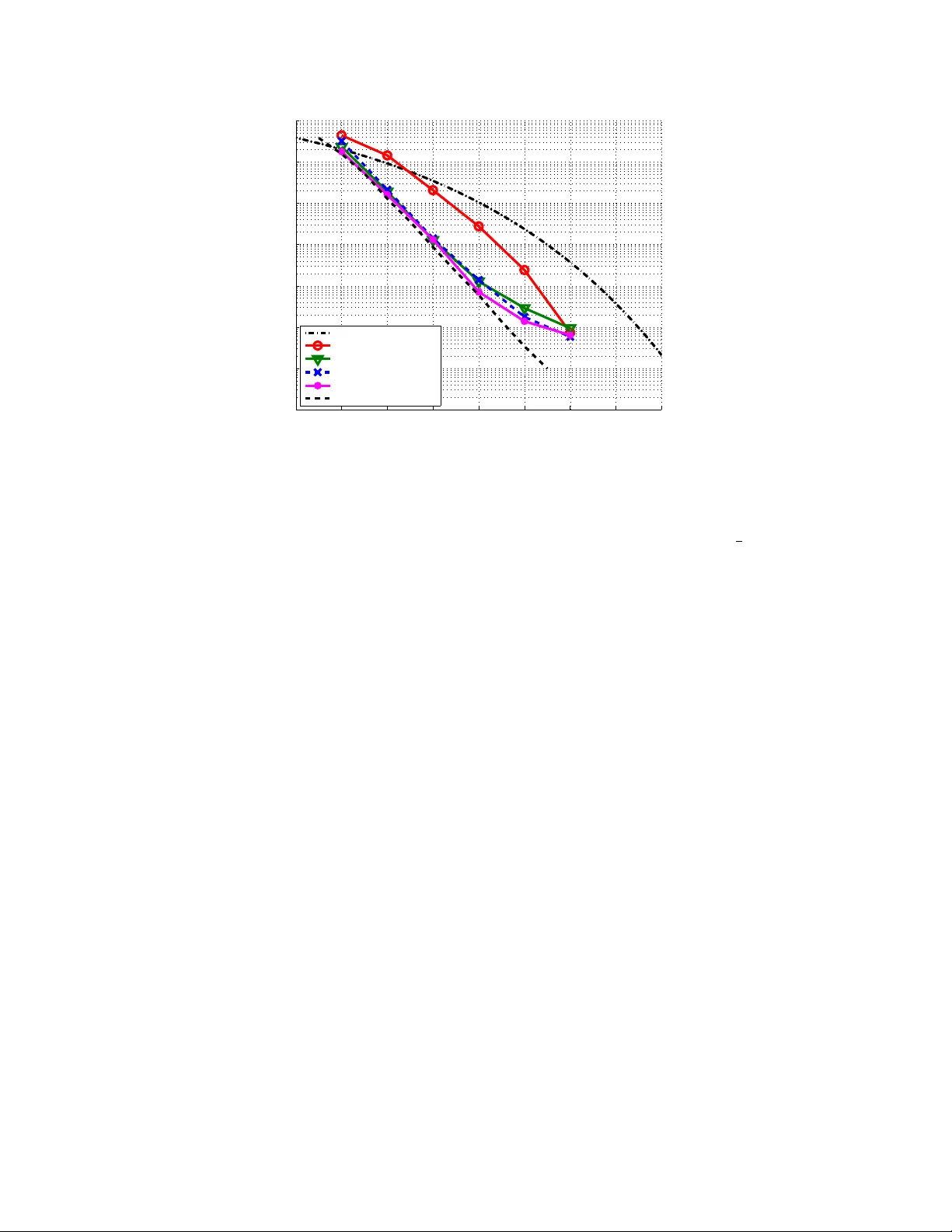
The 30th Symposium on Information Theory and its Applications (SIT A2007) Kashikojima, Mie, Japan, Nov. 27–30, 2007 Message-P assing Deco ding of Lattices Using Gaussian Mixtures Brian M. Kurk oski ∗ Justin Dau wels † Abstract — A lattice deco der which represen ts messages explicitly as a mixture of Gaussians functions is giv en. In order to preven t the num b er of functions in a mixture from gro wing as the deco der iterations progress, a method for replacing N Gaussian functions with M Gaussian functions, with M ≤ N , is given. A squared distance metric is used to select functions for com bining. A pair of selected Gaussians is replaced by a single Gaussian with the same first and second moments. The metric can be computed efficien tly , and at the same time, the prop osed algorithm empirically giv es go od results, for example, a dimension 100 lattice has a loss of 0.2 dB in signal-to-noise ratio at a probability of sym b ol error of 10 − 5 . Keyw ords — Lattice decoding, Gaussian mixtures 1 In tro duction Lattices play a cen tral role in many comm unica- tion problems. While Shannon used a non-lattice, and non-constructiv e, Euclidean-space code to compute the capacit y of the A W GN channel, recently Erez and Za- mir sho wed that lattice enco ding and decoding can also ac hieve the capacity of the A WGN channel [1]. Sim- ilarly , for the problem of communication with known noise, whic h has applications to multiuser comm uni- cations and information hiding, lattice co des play an imp ortan t role [2]. In source co ding, lattices ma y b e used for lossy compression of a real-v alued source. T o approach theoretical capacities, it is necessary to let the dimension of the lattice or co de b ecome asymp- totically large. Ho wev er, for most lattices of interest, the deco der complexity is w orse than linear in the di- mension, and most studied lattices hav e small dimen- sion. F or example, a frequently cited reference on lat- tice deco ding gives experimental results with a maxi- m um dimension of 45 [3]. Other approaches use trellis- based lattices, whic h are exp onen tially complex in the n umber of states [4]. Historically , finite-field error cor- recting co des also suffered the same complexity limita- tion, ho wev er, with the adv ent of iteratively-decoded lo w-density parity chec k co des and turbo codes, the theoretical capacity of some binary-input communica- tion channels can b e achiev ed [5]. Recen tly , a new lattice construction and deco ding algorithm, based up on the ideas of lo w-density parit y c heck codes has b een in tro duced. So-called low-densit y lattice co des (LDLC) are lattices defined by sparse in- v erse generator matrix with a pseudo-random construc- ∗ Dept. of Information and Communications Engineer- ing, Univ. of Electro-Communications, T okyo, Japan, kurkoski@ice.uec.ac.jp. † Amari Research Unit, RIKEN Brain Science Institute, Saitama, Japan, justin@dauw els.com. tion. Deco ding is p erformed iteratively using message- passing, and complexit y is linear in the blo c k length. Sommer, F eder and Shalvi, who prop osed this lattice and deco der, demonstrated deco ding with dimension as high as 10 6 . Ho w ever, the exp eriments considered deco ding only for a sp ecial communications problem where the transmit pow er is unconstrained. Comments in their pap er suggest that the algorithm did not con- v erge when applied to the more important problem of general lattice deco ding [6] [7]. When deco ding on the A WGN channel, the LDLC deco der messages are contin uous-v alued functions, whic h can b e exactly represented by a mixture of Gaus- sian functions. Ho wev er, as iterations progress, the n umber of Gaussians in the mixture grows rapidly . A direct implementation of a deco der whic h exploits this prop ert y is infeasible, and so prior w orks quan tize the messages, ignoring the Gaussian nature of the mes- sages. In this paper, the LDLC deco der messages are rep- resen ted as Gaussian functions, and the growth in the n umber of Gaussians is reduced by a proposed Gaussian mixture reduction algorithm. This algorithm appro xi- mates a n umber of Gaussians N with a smaller n umber of Gaussians M . The algorithm com bines Gaussians in a pair-wise fashion iterativ ely until a stopping con- dition is reac hed. A distance metric, whic h computes the squared difference b et w een a pair of Gaussian func- tions, and the single Gaussian which has the same first and second momen ts, is used. Section 2 gives a review of the construction and de- co ding algorithm for low-densit y lattice co des. If the c hannel noise is Gaussian, then messages in the deco d- ing algorithm can b e represen ted as a mixture of Gaus- sian functions. Section 3 gives a metho d for replacing a pair of Gaussians with a single Gaussian, which is applied to an algorithm which reduces a mixture of N Gaussian functions to a mixture of M Gaussians. Sec- tion 4 applies this algorithm to the decoding of low- densit y lattice co des, and considers sim ulation results. Section 5 is the conclusion. 2 Lo w-densit y Lattice Co des 2.1 Lattices and Lattice Communication A lattice is a regular infinite array of p oin ts in R n . Definition An n -dimensional lattice Λ is the set of p oin ts x = ( x 1 , x 2 , . . . , x n ) with x = G b , (1) where G is an n -b y- n generator matrix and b = ( b 1 , . . . , b n ) is the set of all possible integer v ectors, b i ∈ Z . The following comm unications system is considered. Let the co dew ord x b e an arbitrary p oin t of the lattice Λ. This codeword is transmitted ov er an A WGN chan- nel with known noise v ariance σ 2 , and received as the sequence y = { y 1 , y 2 , . . . , y n } : y i = x i + z i , i = 1 , 2 , . . . , n, (2) where z i is the A W GN. A maxim um-likelihoo d decoder selects b x as the estimated co dew ord: b x = arg max x ∈ Λ P r ( y | x ) (3) The receiv ed codeword is correct if x = b x and incor- rect otherwise. The p o wer of the transmitted sym b ol, || x || 2 is unbounded. Instead, p o wer is restricted b y the v olume of the V oronoi region, det( G ). F or this system, Polt yrev [8] show ed that for suf- ficien tly large n , there exists a lattice for which the probabilit y of error b ecomes arbitrarily small, if and only if, σ 2 < | det( G ) | 2 /n 2 π e . (4) P oltyrev’s result is in contrast to Shannon’s theo- rem that the capacity of the Gaussian channel, sub ject to a transmission p ow er constraint, is 1 2 log(1 + SNR). T o achiev e capacit y while observing the p o wer con- strain t, the co dep oin ts are on the surface of an n -sphere with high probabilit y . 2.2 LDLC Definition Definition A low-densit y lattice co de is a lattice with a non-singular generator matrix G , for whic h H = G − 1 is sparse. Regular LDLC’s ha ve H matrices with constant row and column weigh t d . Although not necessary , it is con venien t to assume that det( H ) = 1 / det( G ) = 1. The non-zero en tries are selected pseudo-randomly . In a magic squar e LDLC , the absolute v alues of the d non-zero entries in each row and eac h column are dra wn from the set { h 1 , h 2 , . . . , h d } with h 1 ≥ h 2 ≥ · · · ≥ h d > 0. The signs of the en tries of H are pseudo- randomly c hanged to min us with probabilit y 0.5. F rom here, ( n, d ) magic square LDLC’s are considered with h 1 = 1, and h i = 1 / √ d for i = 2 , . . . , d . Such co des resulted in only slightly worse p erformance than other w eight sequences [7]. 2.3 LDLC Decoding The LDLC deco ding algorithm is based upon b elief- propagation, where messages are real functions cor- resp onding to probabilit y distributions on the sym- b ols x i . As with deco ding lo w-density parity c heck co des, the deco ding algorithm ma y be presented on a bipartite graph. There are nd v ariable-to-chec k mes- sages q k ( z ), and nd chec k-to-v ariable messages r k ( z ), k = 1 , 2 , . . . , nd . With an A WGN c hannel, the initial message is: q k ( z ) = 1 √ 2 π σ e − ( y i − z ) 2 2 σ 2 , (5) for the edge k connected to v ariable node i . 2.3.1 Chec k No de F or the chec k no de, note that (1) can b e re-written as: H x = b , (6) whic h defines a sparse system of equations: h ij 1 x j 1 + h ij 2 x j 2 + · · · + h ij 1 x j 1 = b i , (7) for i = 1 , 2 , . . . , n , and j k ∈ I i , where I i is the columns of H which ha ve a non-zero entry in p osition i . Let e x k = h k x k , so P d i =1 e x i = b , where b is an in- teger. The input and output messages are q k ( z ) and r k ( z ), respectively , for k = 1 , 2 , . . . , d . F rom (7), for an arbitrary i , x k = b − ( h 1 x 1 + · · · + h k − 1 x k − 1 + h k +1 x k − 1 + · · · + h d x d ) h k , or, x k = 1 h k ( b − d \ k X i =1 e x i ) . (8) The output message r k ( z ) can b e obtained from the input messages q i ( z ) , i = 1 , . . . , d, i 6 = k in four steps, Unstretc h, Con volution, Extension and Stretch. Unstr etch is multiplication b y h k . The message for e x i is e q k ( z ), e q k ( z ) = q k ( z h k ) . (9) Convolution The message for P d \ k i =1 e x i is e r k ( z ). The distribution of the sum of random v ariables is the con- v olution of distributions, e r k ( z ) = ( e q 1 ∗ · · · ∗ e q k − 1 ∗ e q k +1 ∗ · · · ∗ e q d )( z ) , (10) where ∗ denotes real-num b er conv olution. Extension is a shift-and-rep eat op eration for the un- kno wn in teger b . Conditioned on a sp ecific v alue of b , the distribution of b − P d \ k i =1 e x i is e r k ( b − z ). Assum- ing that b is an arbitrary integer w ith uniform a priori distribution, e r 0 k ( z ) = ∞ X b = −∞ e r k ( b − z ) . (11) Str etching is multiplication b y 1 /h k . Finally the message r k ( z ) which is the message for (8), is obtained as: r k ( z ) = e r 0 k ( h k z ) (12) Note that the ab o v e op erations are linear and can b e in terchanged as is required for an implemen tation. 2.3.2 V ariable No de A t v ariable no de i , tak e the product of incoming messages, and normalize. Pr o duct: b q k ( z ) = e − ( y i − z ) 2 2 σ 2 d \ k Y i =1 r i ( z ) . (13) Normalize: q k ( z ) = b q k ( z ) R ∞ −∞ b q k ( z ) dz . (14) 2.3.3 Estimated Co dew ord and Integer Se- quence The chec k node and v ariable no de op erations are re- p eated iterativ ely until a stopping condition is reac hed. Estimate the transmitted by co dew ord b x by first com- puting the a posteriori message F i ( z ) for the code sym- b ol x i as: F i ( z ) = e − ( y i − z ) 2 2 σ 2 d Y k =1 r k ( z ) . (15) Find b x i as: b x i = arg max z ∈ R F i ( z ) . (16) The estimated in teger sequence b b is: b b = h H b x i , (17) where h z i denotes the integer closest to z . 2.4 Gaussian Mixture Decoder When the c hannel noise is Gaussian, all of the LDLC messages can be describ ed as a mixture of Gaus- sian functions. F rom here, “Gaussians” will b e used as shorthand for “Gaussian functions”. In this section, it is assumed that a message f ( z ) is a mixture of N Gaussians, f ( z ) = N X i =1 c i N ( z ; m i , v i ) , (18) where c i ≥ 0 are the mixing coefficients with P N i =1 c i = 1, and N ( z ; m, v ) = 1 √ 2 π v e − ( z − m ) 2 2 v . (19) In this w ay , the message f ( z ) can b e describ ed b y a list of triples of means, v ariances and mixing co efficien ts, { ( m 1 , v 1 , c 1 ) , . . . , ( m N , v N , c N ) } In describing the Gaussian mixture deco der, ini- tially assume that the input messages to a node consist of a single Gaussian, that is N = 1. Che ck no de Without loss of generalit y , consider c heck no de inputs k = 1 , 2 , . . . , d − 1 and output d . Each input message q k ( z ) is a single Gaussian N ( z ; m k , v k ). The message e q k ( z ) is obtained b y multiplying b y h k , so e q k ( z ) = N  z ; h k m k , h 2 k v k  . The message e r d ( z ) is the conv olution of e q k ( z ) , k = 1 , . . . , d − 1. So: e r d ( z ) = N z ; d − 1 X k =1 h k m k , d − 1 X i =1 h 2 k v k ! . (20) The message e r 0 d ( z ) is e r d ( z ) shifted ov er all p ossible in tegers: e r 0 d ( z ) = ∞ X b = −∞ N z ; d − 1 X k =1 h k m k + b, d − 1 X k =1 h 2 k v k ! . The output message r d ( z ) is obtained by scaling by − 1 /h d , so: r d ( z ) = ∞ X b = −∞ N z ; − P d − 1 k =1 h k m k + b h d , P d − 1 k =1 h 2 k v k h 2 d ! . V ariable No de . Let the chec k-to-v ariable no de mes- sages r k ( z ) , k = 1 , . . . , d − 1 b e Gaussians N ( z ; m k , v k ). F or notational conv enience, let m 0 = y i b e the symbol receiv ed from the channel at no de i and let v 0 = σ 2 b e the channel v ariance, as in (5). The output message q d ( z ), the pro duct of these input messages, will also be a Gaussian, q d ( z ) = k d N ( z ; m d , v d ) , (21) where, 1 v d = d − 1 X k =0 1 v k , (22) m d v d = d − 1 X k =0 m k v k (23) and, k d = r v d (2 π ) d − 2 Q i v i exp  − v d 2 d − 2 X i =0 d − 1 X j = i +1 ( m i − m j ) 2 v i v j  . F or the general case where the input consists of a mixture of Gaussians, at either the chec k no de or the v ariable no de, the output can be found by conditioning on one elemen t from eac h input mixture and comput- ing a single output Gaussian. The mixing coefficient for this Gaussian is the pro duct of the input mixing co ef- ficien ts. Then the output is the mixture of these single Gaussians created b y conditioning all input combina- tions. The num b er of Gaussians in each mixture gro ws rapidly as the iterations progress. A t the v ariable no de, if input k consists of a mixture of N k Gaus- sian functions, then the output message will consist of N 1 N 2 · · · N d − 1 Gaussian functions. At the chec k no de, ev en if the num b er of in teger shifts is b ounded, the n umber of Gaussian functions in the mixture also gro ws as O ( N d − 1 ). A naiv e implemen tation of this Gaussian mixture deco der is prohibitively complex. The follow- ing section prop oses a technique for approximating a large num b er of Gaussians. 3 Gaussian Mixture Reduction This section describ es an algorithm whic h approxi- mates a mixture of Gaussian functions with a smaller n umber of Gaussian functions. The algorithm input is a mixture of N Gaussians, f ( z ), as defined in (18), given as a list of triples. The algorithm output is a list of M triples of means, v ariances and mixing co efficients, { ( m m 1 , v m 1 , c m 1 ) , . . . , ( m m M , v m M , c m M ) } with P M i =1 c m i = 1, that similarly forms a Gaussian mixture g ( z ). With M ≤ N , the output mixture should b e a go od appro ximation of the input mixture: f ( z ) ≈ g ( z ) = M X i =1 c m i N ( z ; m m i , v m i ) . (24) First, a metric which describ es the error due to re- placing a t wo Gaussians with a single Gaussian is given. Then, this is incorporated in to a greedy search algo- rithm which replaces N Gaussians with M Gaussians. 3.1 Appro ximating a Mixture of Two Gaus- sians with a Single Gaussian Definition The squared difference SD( p || q ) b etw een t wo distributions p ( z ) and q ( z ) with supp ort Z is de- fined as: SD( p || q ) = Z z ∈Z ( p ( z ) − q ( z )) 2 dz (25) L emma The squared difference SD( p || q ) has the fol- lo wing prop erties: • SD( p || q ) ≥ 0 for any distributions p and q . • SD( p || q ) if and only if p = q . • SD( p || q ) = SD( q || p ). L emma The squared difference b etw een the Gaus- sian distributions N ( m 1 , v 1 ) and N ( m 2 , v 2 ) is given b y SD( N ( m 1 , v 1 ) , N ( m 2 , v 2 )) = 1 2 √ π v 1 + 1 2 √ π v 2 − 2 p 2 π ( v 1 + v 2 ) e − ( m 1 − m 2 ) 2 2( s 1 + s 2 ) . (26) L emma The squared difference betw een a single Gaussian N ( m, v ) and a mixture of tw o Gaussians c 1 N ( m 1 , v 1 ) + c 2 N ( m 2 , v 2 ), with c 1 + c 2 = 1, is: 1 2 √ π v + c 2 1 2 √ π v 1 + c 2 2 2 √ π v 2 − 2 c 1 p 2 π ( v + v 1 ) e − ( m − m 1 ) 2 2( v + v 1 ) − 2 c 2 p 2 π ( v + v 2 ) e − ( m − m 2 ) 2 2( v + v 2 ) + 2 c 1 c 2 p 2 π ( v 1 + v 2 ) e − ( m 1 − m 2 ) 2 2( v 1 + v 2 ) . (27) There is unfortunately no closed-form expression for the minimal squared difference in the previous lemma. Ho wev er, minimizing the Kullbac k-Leibler divergence b et w een the single Gaussian distribution and the mix- ture of t wo Gaussian distributions is tractable; it sim- ply amoun ts to momen t matching. Therefore, from no w w e will consider the moment-matc hed Gaussian appro ximation. L emma The mean m and v ariance v of a mixture of t wo Gaussian distributions c 1 N ( m 1 , v 1 ) + c 2 N ( m 2 , v 2 ) are given by: m = c 1 m 1 + c 2 m 2 (28) s = c 1 ( m 2 1 + v 1 ) + c 2 ( m 2 2 + v 2 ) − c 2 1 m 2 1 − 2 c 1 c 2 m 1 m 2 − c 2 2 m 2 2 . (29) Let t i , i = 1 , 2 denote the triple ( m i , v i , c i ), where c 1 + c 2 is not necessarily one, and let the normalized triple be t i = ( m i , v i , c i / ( c 1 + c 2 )). The single Gaussian whic h satisfies the prop ert y of the Lemma is denoted as: t = MM( t 1 , t 2 ) , (30) where t = ( m, v , 1), with m and v as giv en in (28) and (29). Definition The Gaussian quadratic loss GQL( p ) of a probability distribution p is defined as the squared difference b et ween p and the Gaussian distribution with the same mean m and v ariance v as p : GQL( p ) = SD( p k N ( m, s )) . (31) Cor ol lary The Gaussian quadratic loss of a mixture of tw o Gaussian distributions, GQL( t 1 , t 2 ) = SD( c 1 N ( m 1 , v 1 ) + c 2 N ( m 2 , v 2 ) kN ( m, v )) , is obtained ev aluating (27), with m and v as giv en in (28) and (29). 3.2 Appro ximating N Gaussians with M Gaus- sians Here, w e use the results from the previous subsec- tion and prop ose an algorithm which approximates a mixture of N Gaussians with a mixture of N Gaussians. Input: list L = { t 1 , t 2 , . . . , t N } of N triples describ- ing a Gaussian mixture, and tw o stopping parameters, θ the allow able one-step error (measured by GQL) and M , the maximum num b er of allo w able Gaussians in the output. A lgorithm 1. Initialize the curren t searc h list, C , with the input list: C ← L . 2. Initialize the current error, θ c , to the minimum GQL b et ween all pairs of Gaussians: θ c = min t i ,t j ∈C ,i 6 = j GQL( t i , t j ) . 3. Initialize length of current list, M c = N . 4. While θ c < θ or M c > M : (a) Determine the pair of Gaussians ( t i , t j ) with the smallest GQL: ( t i , t j ) = arg min t i ,t j ∈C ,i 6 = j GQL( t i , t j ) . (b) Add the single Gaussian with the same mo- men t as t i and t j to the list: C ← C ∪ M M ( t i , t j ) . (c) Delete t i and t j from list: C ← C \ { t i , t j } . (d) Recalcuate the minim um GQL: θ c = min t i ,t j ∈C ,i 6 = j GQL( t i , t j ) . (e) Decremen t the current list length: M c ← M c − 1. 5. Algorithm output: list of triples C Note that t w o conditions m ust b e satisfied for the algorithm to stop. That is, the one-step error ma y b e greater than the threshold θ if the minimum num b er of Gaussians is not yet met. On the other hand, the n umber of output Gaussians ma y be less than M , if the one-step error is sufficiently low. 4 Gaussian-Mixture Reduction Applied to LDLC Deco ding In this section, the Gaussian mixture reduction al- gorithm of Section 3 is applied to the LDLC deco ding algorithm describ ed in Section 2.4. A t the chec k no de, observe that the message e r k ( z ), as giv en in (10), can b e computed recursively with a k ( z ) and b k ( z ) defined as: a 1 ( z ) = e q 1 ( z ) , (32) a k ( z ) = a k − 1 ( z ) ∗ e q k ( z ) , k = 2 . . . , d − 1 , (33) and, b d ( z ) = e q d ( z ) , (34) b k ( z ) = b k +1 ( z ) ∗ e q k ( z ) , k = d − 1 , . . . , 2 . (35) Then e r k ( z ) is found using a v ariation on the forw ard- bac kward algorithm as: e r 1 ( z ) = b 2 ( z ) , (36) e r k ( z ) = a k − 1 ( z ) ∗ b k +1 ( z ) , k = 2 , 3 , . . . , d − 1 and, (37) e r d ( z ) = a d − 1 ( z ) . (38) The Gaussian mixture reduction algorithm is ap- plied after the computation (33) and (35), for each k . F or example if a k ( z ) is the mixture pro duced b y apply- ing the Gaussian mixture reduction algorithm to a k ( z ), a k ( z ) = GMR( a k ( z )) , (39) then the forw ard recursion of the chec k node function ma y b e stated as: a 1 ( z ) = e q 1 ( z ) , (40) F or k = 2 , 3 , . . . , d − 1: a k ( z ) = a k − 1 ( z ) ∗ e q k ( z ) , (41) a k ( z ) = GMR( a k ( z )) , (42) and similarly for the backw ard recursion. Similarly at the v ariable node, the pro duct (13) can b e decomposed into a forw ard and backw ard rec ursion. In this case as well, the Gaussian mixture reduction algorithm is applied after each step of the recursion. In the Gaussian mixture reduction algorithm, it is desirable to rep eat step 4 as long as the current re- duced Gaussian function g ( z ) (represented b y C ) re- mains a go od approximation of the input function f ( z ) (represen ted b y L ). In practice, it was found that us- ing a “local” stopping condition of a threshold on the one-step error was sufficien t to giv e a go od “global” ap- pro ximation f ( z ) ≈ g ( z ). In many cases, f ( z ) w as w ell- appro ximated by a single Gaussian, whic h was found b y the prop osed algorithm. Ho wev er, using an error threshold alone does not alw ays restrict the n umber of output Gaussians, an im- p ortan t goal of the mixture reduction algorithm. Thus, a second stopping condition, whic h requires that the n umber of Gaussians b e lo wer than some fixed thresh- old, is also enforced. Thus, the Gaussian combining ma y con tinue while M c > M , ev en if the one-step er- ror threshold has b een exceeded. In practice, this did not app ear to hav e a detrimental result for a wide range of symbol-error rates. Sim ulation results comparing the prop osed deco der with the quantized decoder [7] are shown in Fig. 1. A LDLC with n = 100 , d = 5 was used. The sym b ol error rate of a cubic lattice used for transmission is la- b eled “Unco ded.” The horizontal axis is the difference b et w een the channel noise v ariance and the P olt yrev capacit y , 1 / 2 π e , in dB. F or the parameter selection θ = 0 . 5 , 1 . 0, and M ≤ 6, it was found that the prop osed algorithm p erformed with a slight p erformance loss when the probability of sym b ol error w as greater than 10 − 5 . F or example, with θ = 0 . 5 and M = 6, the loss at a sym b ol error rate of 10 − 5 is less than 0.1 dB. F or low er sym b ol error rates, an error floor app ears. It may b e helpful to con- sider this error flo or as analogous to quantization error flo ors whic h app ear in the deco ding of low-densit y par- it y c heck co des when insufficien t quan tization lev els are used. Complexity In the Gaussian mixture reduction al- gorithm, the primary complexity is computing the ini- tial error, which requires computing the GQL b et ween N pairs, a complexity of O ( N 2 ). In the Gaussian mixture deco der, the primary complexit y the pairwise- computation of the outputs, which is O ( M 2 ). These 0 1 2 3 4 5 6 7 8 10 − 8 10 − 7 10 − 6 10 − 5 10 − 4 10 − 3 10 − 2 10 − 1 Distance from Capacity (dB) Prob. of symbol error Uncoded GM decoder, θ =0.5,M=2 GM decoder, θ =0.5,M=3 GM decoder, θ =1,M=6 GM decoder, θ =0.5,M=6 Quantized decoder Figure 1: Symbol error rate of prop osed Gaussian mixture (GM) deco der vs. quantized decoder for n = 100, d = 5. n umbers N and M are random v ariables which dep end up on the nature of the messages, and the effective- ness of the Gaussian mixture reduction algorithm. In the simulations the maxim um v alue of M w as 6, and N ≤ kM 2 , where k is the constan t num b er of in te- ger shifts, k = 3 was used in the simulations. On the other hand, the complexity of the quantized algorithm is dominated b y a discrete F ourier transform of size 1 / ∆ where ∆ is the quan tization bin width, ∆ = 1 / 128 w as used in the simulations. It is difficult to directly mak e comparisons of the computational complexity of the tw o algorithms. The memory required for the prop osed algorithm, ho wev er, is significantly sup erior. The prop osed al- gorithm requires storage of 3 M (for the mean, v ari- ance and mixing co efficien t), for each message, where M ≤ 6. The quan tized algorithm, ho wev er used 1024 quan tization p oin ts for each message. 5 Conclusion LDLC co des can b e used for comm unication o ver unconstrained pow er c hannels. In this paper, we pro- p osed a new LDLC deco ding algorithm which exploits the Gaussian nature of the deco der messages. The core of the algorithm is a Gaussian mixture reduction metho d, whic h appro ximates a message by a smaller n umber of Gaussians. As a result, the LDLC algo- rithm whic h trac ks the means, v ariances and mixing co efficien ts of the comp onen t Gaussians, rather than using quantized messages, was tractable. It was shown b y computer simulation that this algorithm p erforms nearly as well as the quantized algorithm, when the dimension is n = 100, and the probability of symbol error is greater than 10 − 5 . References [1] U. Erez and R. Zamir, “Ac hieving 1 2 log(1 +SNR) on the A WGN channel with lattice enco ding and de- co ding,” IEEE T r ansactions on Information The- ory , vol. 50, pp. 2293–2314, Octob er 2004. [2] U. Erez, S. S. (Shitz), and R. Zamir, “Capacity and lattice strategies for canceling kno wn in terference,” IEEE T r ansactions on Information The ory , v ol. 51, pp. 3820–3833, No vem b er 2005. [3] E. Agrell, T. Eriksson, A. V ardy , and K. Zeger, “Closest p oin t search in lattices,” IEEE T r ansac- tions on Information The ory , v ol. 48, pp. 2201– 2214, August 2002. [4] U. Erez and S. ten Brink, “A close-to-capacit y dirt y pap er co ding sc heme,” IEEE T r ansactions on In- formation The ory , v ol. 51, pp. 3417–3432, Octob er 2005. [5] T. J. Richardson, M. A. Shokrollahi, and R. L. Urbank e, “Design of capacity-approac hing irregu- lar lo w-density parit y-c heck codes,” IEEE T r ansac- tions on Information The ory , vol. 47, pp. 619–637, F ebruary 2001. [6] N. Sommer, M. F eder, and O. Shalvi, “Low densit y lattice co des,” in Pr o c e e dings of IEEE International Symp osium on Information The ory , (Seattle, W A, USA), IEEE, July 2006. [7] N. Sommer, M. F eder, and O. Shalvi, “Low densit y lattice co des.” submitted to IEEE T ransaction on Information Theory . Av ailable h [8] G. Polt yrev, “On coding without restrictions for the a wgn c hannel,” IEEE T r ansactions on Information The ory , vol. 40, pp. 409–417, March 1994.