Efficient l_{alpha} Distance Approximation for High Dimensional Data Using alpha-Stable Projection

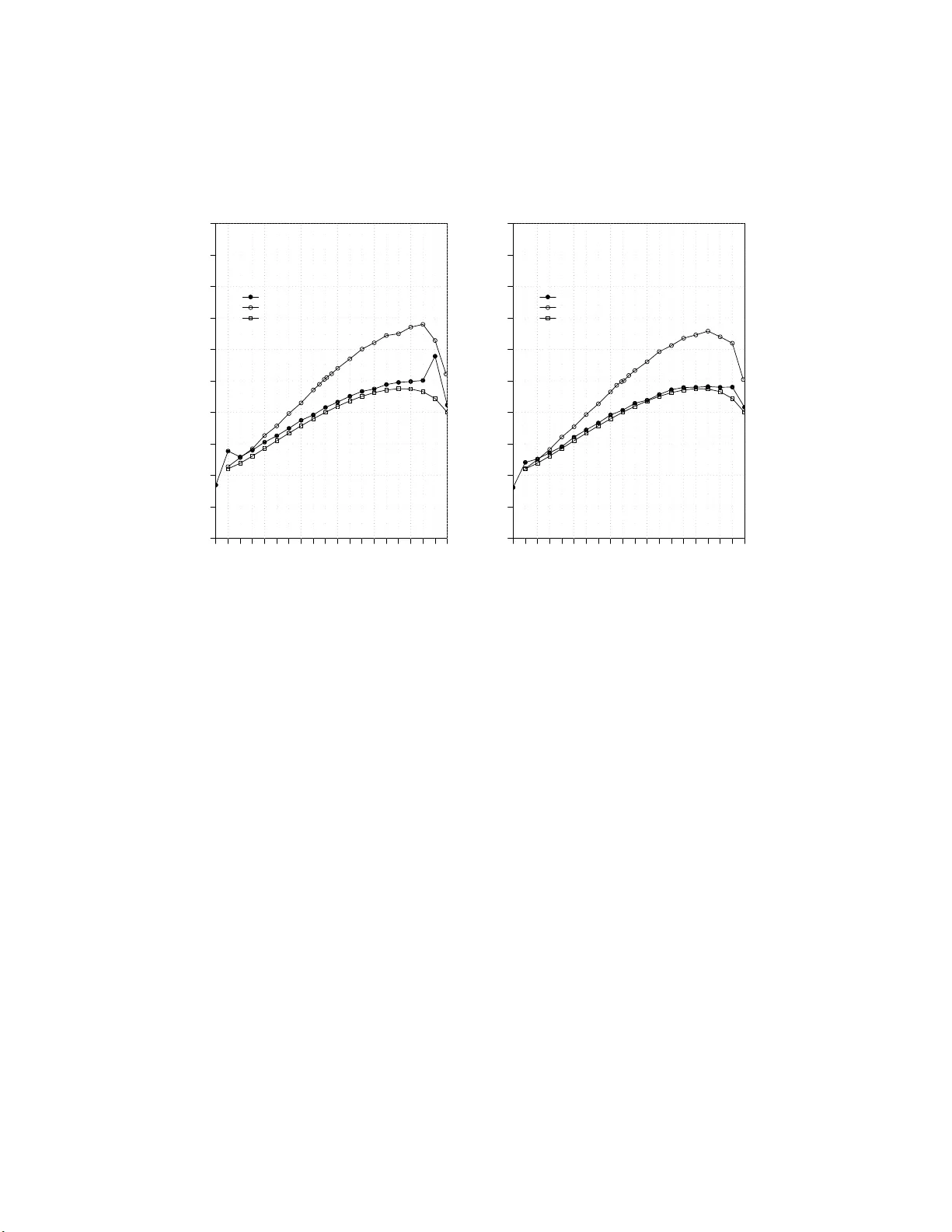
Efficien t l α Distance Appro ximation for High Dimensional Data Usi ng α -Stable Pro jection Peter Clifford and Ioana Ada Cosma Department of Statistics, Un ivers it y of Ox ford 1 S outh Parks Road, Ox ford OX1 3TG, U nited Kin gd om { cliffor d,c osma } @stats.ox.ac.uk Abstract. In recent years , large high-dimensional data sets have b ecome com- monplace in a wide range of applications in science and commerce. T ec hniqu es for dimension reduction are of p rimary concern in statistical analysis. Pro jection metho d s play an imp ortant role. W e inv estigate the use of pro jection algorithms that exploit prop erties of the α -stable d istribu t ions. W e show that l α distances and quasi-distances can be recov ered from rand om pro jections with full statis tical efficiency by L-estimation. The computational requirements of our algorithm are mod est; after a once-and - for-all calculation to determine an array of length k , the algorithm runs in O ( k ) time for eac h distance, where k is the reduced dimension of the pro jection. Keywords: random pr o jections, stable distribution, L- e stimation 1 In tr o duction Let V be a co llection of n points in m -dimensional Euclidean s pace, R m , where the dimension m is large, of the order of h undreds or thousands. W e are int erested in distance-preser ving dimension reduction via random pro jections, where the p oints in V are r andomly pro jected onto a low er k -dimensional space such that pairwise dista nces b etw een orig inal points ar e well preser ved with high a ccuracy . Statistical a nalyses based on pairwise dis tances b etw een po ints in V can b e p erfor med on the set of pro jected p oints, thu s re duc- ing the computationa l cost of computing all pairwise distance s from O ( n 2 m ) to O ( nmk + n 2 k ). Imp ortant applica tions of distance-pr eserving dimens io n reduction are approximate c lustering in high dimensiona l spac e s and compu- tations ov e r str eaming data, for exa mple Hamming dista nce approximations. W e consider the problem of preserving l α distances (quasi-distances) de- fined by d α ( u, v ) = P m i =1 | u i − v i | α , for ( u 1 , . . . , u m ) and ( v 1 , . . . , v m ) ∈ R m , for α ∈ (0 , 2]. W e rema r k t hat [ d α ( u, v )] 1 /α is a distance measure for α ≥ 1, but not for α < 1 , a nd that the Hamming distance is obtained as lim α → 0 d α ( u, v ). In the case α = 2, the lemma of Johnson and Lindenstrauss (1984) demon- strates the existence o f a pro jection map p α : R m 7→ R k such that (1 − ǫ ) d α ( u, v ) ≤ d α ( p α ( u ) , p α ( v )) ≤ (1 + ǫ ) d α ( u, v ) ∀ u, v ∈ V , (1) 2 Clifford, P . and Co sma, I. A. provided that k ≥ k 0 = O (log n/ǫ 2 ). W e are in ter ested in dimensio n reduction in l α , for general α ∈ (0 , 2], using stable rando m pro jections. See Indyk (2006) fo r an introduction to this technique. The goal will b e to satisfy the inequality in (1) with hig h probability . In Section 2 we define sta ble r andom pr o jections, and show that distance preserv ing dimensio n r eduction in l α reduces to estimation of the scale pa rameter of the symmetric, strictly stable law, where the latter is discussed in Sectio n 3. In Sectio n 4 we pre sent an asymptotically efficien t estimator of the scale pa rameter, followed by numerical results in Section 5. 2 Random pro jections A rando m v ariable X with distr ibution F is said to b e strictly st able if for every n > 0, and independent v ariables X 1 , . . . , X n ∼ F , ther e exist co n- stants a n > 0 such that X 1 + . . . + X n D = a n X , wher e D denotes equality in distribution. The only p ossible no r ming constants a re a n = n 1 /α , where 0 < α ≤ 2; the parameter α is kno wn as the inde x of stability (F eller , 197 1). The densities of s table distributions are no t a v aila ble in closed form, except in a few cas e s: Cauch y ( α = 1), Nor mal( α = 2) and L ´ evy( α = 0 . 5). W e are interested in s y mmetric, strictly s table random v ariables of index α and para meter θ > 0, with character istic function E exp( itX ) = e − θ | t | α , defined for t real. Let f ( x ; α, θ ) and F ( x ; α, θ ) b e the densit y and distribution function of X . Of par ticula r in teres t is the following pro per ty . Suppos e that X 1 , . . . , X m are independent v ar iables with distribution function F ( x ; α, 1) and that u 1 , . . . , u m are rea l cons tants, then P m i =1 u i X i ∼ F ( x ; α, θ ) where θ = P d i =1 | u i | α . If v 1 , . . . , v m is another seque nc e o f rea l constants, then it follows that P m i =1 ( u i − v i ) X i ∼ F ( x ; α, θ ) with θ = d α ( u, v ). W e assume that the da ta V is a rrange d into a matr ix V with n rows and m columns, i.e. o ne row fo r each of the n data p oints. Let X ∈ R m × k be a matrix whos e entries ar e indep endent sy mmetric, strictly stable ra ndo m v ariables with index α , and θ = 1 for fixed 0 < α ≤ 2. W e term X a r andom pr oje ction matrix mapping from R m to R k via the map V 7→ VX . Let B = VX and cons ider u and v , the i th a nd j th r ows of V , i 6 = j , corresp onding to the i th a nd j th data p oints in V . Let a and b b e the corres p o nding rows o f B . Then, for z = 1 , . . . , k , w e hav e a z − b z = m X l =1 ( u l − v l ) X lz ∼ F ( x ; α, d ij ) , independently for z = 1 , . . . , k , where d ij = d α ( u, v ). Our a im is to recov er d α ( u, v ) from ( a, b ). Since { a z − b z : z = 1 , . . . , k } provides a sample o f v a lues from a distribution with parameter d α ( u, v ) we a re in a po sition to apply the usual r ep e r toire of sta tis tica l es- timation techniques to obtain estimators with sp ecified accuracy . This is of particular relev ance in the context of streaming data, where d α , for α ≤ 1, Efficien t l α Distance A pproximation for H igh Dimensional Data 3 is a meaningful measure o f the pair wise distance b etw een streams; in the extreme case o f α → 0, d α tends to the Hamming distance, the num b er of mismatches b etw een tw o seq uences. When α ∈ [1 , 2], the l α distance is g iven by d 1 /α α with po tent ial interest for clustering in high dimensiona l spaces. In the case α ∈ [1 , 2 ] the s tatistical pr oblem reduces to estimating the sta ndard scale pa rameter of the symmetric, strictly stable la w. 3 Estimation of the scale parameter The pro blem of parameter estimatio n of the stable law is par ticularly chal- lenging due to the fact that the dens ity function does not exist in c lo sed for m for most v alues of α ∈ (0 , 2]. The c a ses α = 1 and α = 2 hav e b een ex- tensively studied. See for ex ample (Li et al., 2007) for r eferences. Ma ximum likelihoo d es timation of the par ameters was first attempted in DuMouchel (1973) who show ed that the MLE’s ar e b o th consistent and asymptotically normal, and co mputed estimates of the asymptotic standard deviations a nd correla tions. Ma tsui and T akemu ra (2006) impr oved up on these estima tes by providing accura te approximations to the first a nd second deriv atives of the stable densities. Nolan (200 1) pro p oses an iterative appr oach to maximum likelihoo d estimation of the parameters , implemented in his soft ware pack age ST ABLE, av ailable a t http://www.robustanalysis .com/. W e co mpute approximations to the second deriv ative of the stable density and the log arithm of a tr ansformed density b y a seco nd or der finite difference scheme with gr id w idth h = 0 . 01 using the integral for m of the density func- tion given in Nolan (2007), as implemen ted in the cont ributed pac k age fBasics to R; Figure 1 displays the approximations. W e obtained similar estimates using the expressions in Matsui and T akem ura (2006). Among the first estimators of the s c a le parameter ar e tho se of F a ma and Roll (196 8) bas ed on sample qua nt iles, for α > 1. The known fo rm of the characteristic function o f the stable law has pr ov ed to be a use ful to o l for parameter estimation (Ko gon and Williams, 1998). More recent ly , Li (200 8 ) prop oses the harmonic mean estimator for α ≤ 0 . 344 and the geometric mean estimator for 0 . 344 < α < 2 to estimate θ ; combined, these estimators hav e an asymptotic rela tive efficiency ex c eeding 7 0 % and increasing to 100% as α → 0. F urthermo re, Li a nd Ha stie (2008) pr op ose a unified estimator based on fractional p ow ers with ARE no smaller than 75 %, out-p erforming the combined harmonic and geo metric mean estimator s, and with g o o d small sample p erforma nce for v alues of k as small as 10; we p oint o ut that the fractional p ow e r estimator has b een pro po sed pre v iously in Nikia s and Shao (1995). O ur a pproach is to us e L-estimatio n to estimate the lo garithm of the scale par ameter. W e will show that the metho d is simple and practica l, inv olving only a precalculated table and then a subsequent s um of pro ducts to ac hieve a symptotic efficiency of 10 0%. 4 Clifford, P . and Co sma, I. A. −0.4 −0.2 0.0 0.2 0.4 −400 −200 0 200 400 x alpha=0.1 alpha=0.2 alpha=0.3 alpha=0.4 alpha=0.5 −2 −1 0 1 2 −10 −5 0 x alpha=0.6 alpha=0.7 alpha=0.8 alpha=0.9 alpha=1.0 −4 −2 0 2 4 −0.6 −0.4 −0.2 0.0 0.2 x alpha=1.1 alpha=1.2 alpha=1.3 alpha=1.4 alpha=1.5 −4 −2 0 2 4 −0.3 −0.2 −0.1 0.0 0.1 x alpha=1.6 alpha=1.7 alpha=1.8 alpha=1.9 alpha=2.0 Fig. 1. Approximations to the second deriv ativ e of f ( x ; α, 1) for α ∈ [0 . 1 , 2]. 4 The approac h of L-estimation Consider a random sample x 1 , . . . , x k ∼ f ( x ; α, θ ) and let γ = θ 1 /α . Define y i := lo g | x i | D = µ + z i , i = 1 , . . . , k , where z i is distributed a s the logarithm of the abso lute v a lue of a symmetric, strictly stable r andom v ar iable of index α and θ = 1, a nd µ = lo g γ . Let f 0 ( z ) and F 0 ( z ) deno te the p.d.f. and distribution function of z i , resp e c tively . So , ( y 1 , . . . , y k ) is a ra ndom sa mple of v ariables with p.d.f. f 0 ( y − µ ), where f 0 ( z ) = 2 e z f ( e z ; α, θ ) , −∞ < z < ∞ . The problem r educes to that of estimating the lo ca tion para meter µ fo r the family of distributions { f 0 ( y − µ ) , µ ∈ R } , bas e d on a r andom sample ( y 1 , . . . , y k ) fro m f 0 ( y − µ ). The metho d of L-estimation defines the estimate ˆ µ as a weigh ted linear combination of or der statistics y (1) , . . . , y ( k ) . Cherno ff et al. (19 67) prove that when the weigh ts are suitably chosen , √ k ( ˆ µ − E ( ˆ µ )) is asymptotica lly nor- mal with mean 0 and v ar iance I − 1 µ . Co nsequently the estimator ˆ µ is asy mp- totically efficient. Efficien t l α Distance A pproximation for H igh Dimensional Data 5 In larg e samples , the weigh ts ca n b e approximated by w ik = − 1 k I µ ℓ ′′  F − 1 0  i k + 1  , (2) where ℓ ( y ) = log f 0 ( y ). F urthermo re, the s y stematic bia s-corr ection term is given by B C = E ( ˆ µ ) − ˆ µ = − 1 I µ Z ∞ −∞ z ℓ ′′ ( z ) f 0 ( z ) dz , so, the corresp onding bias-cor rected e s timator is ˆ µ B C = P k i =1 w ik y ( i ) − B C . T able 1 gives the Fisher information and the bias for v ar ious v alues of α , obtained numerically by mak ing use of appr oximations to the stable densities and quant iles in the R pack ag e fBasics. The v a lues of Fis her information agree with those presen ted b y Matsui and T akem ura (2006) to within 3-4 significan t digits for α ∈ (0 . 3 , 1 . 8), but appear to b e slightly differe nt for α outside this range; for example, for α = 1 . 8, our estimate is 1.3920, whereas that of Matsui and T a kem ura (20 06) is 1.3898. α I µ B C α I µ B C α I µ B C α I µ B C 0.14 0 0.0183 -1.5253 0.6 0.2325 - 0.4380 1.1 0.5774 0.0762 1.6 1.0780 0.4183 0.15 0.0 210 -1.452 2 0.65 0.2626 -0.3658 1.15 0.6182 0.1119 1.65 1.1459 0.4497 0.2 0.0363 -1.1956 0.7 0.2937 -0.2995 1.2 0.6604 0.1466 1.7 1.2198 0.4741 0.25 0.0 547 -1.042 0 0.75 0.3256 -0.2388 1.25 0.7042 0.1804 1.75 1.3011 0.4874 0.3 0.0755 -0.9331 0.8 0.3585 -0.1834 1.3 0.7499 0.2138 1.8 1.3920 0.4875 0.35 0.982 -0.8438 0.85 0.3924 -0.1324 1.35 0.7976 0.2470 1.85 1.4968 0.4743 0.4 0.1226 -0.7611 0.9 0.4272 -0.0852 1.4 0.8476 0.2804 1.9 1.6270 0.4480 0.45 0.1 483 -0.679 0 0.95 0.4631 -0.0412 1.45 0.9002 0.3142 1.95 1.7882 0.4122 0.5 0.1753 -0.5965 1.0 0.5 0 1.5 0.9558 0.3487 1.99 1.8861 0.3912 0.55 0.2 034 -0.515 4 1.05 0.5379 0.0390 1.55 1.0148 0.3838 2.0 2. 0 0.3687 T able 1. Fisher information I µ for the parameter µ and t he systematic bias (BC) in estimating µ by efficient L-estimation, tabulated for v alues of α ∈ [0 . 14 , 2]. In the case α > 1 we will b e interested in estimating γ = e µ , corr e- sp onding to the l α norm. W e prop ose the estimator ˆ γ = exp ( ˆ µ B C ). It follows that √ k  ˆ γ − γ  is asy mptotica lly nor mal with mean 0 and v ariance 1 /I γ , where I γ is the Fisher information ab out the sca le parameter γ contained in ( x 1 , . . . , x k ), or eq uiv alently ( y 1 , . . . , y k ). By second order T a ylor e x pansion, we show that the bias incurred by ex po nentiating is approximately E ( ˆ γ ) ≈ γ + 1 2 γ E ( ˆ µ B C − µ ) 2 = γ  1 + 1 2 k I µ  , so the bias-cor rected estima to r ˆ γ B C = ˆ γ  1 − 1 2 kI µ  is unbiased up to terms of o rder O (1 /k 2 ). 6 Clifford, P . and Co sma, I. A. 0.0 0.2 0.4 0.6 0.8 1.0 0.00 0.01 0.02 0.03 t normalised weight alpha=0.15 alpha=1.0 alpha=2.0 Fig. 2. T h is plot d ispla y s ap p roxima te weigh ts w ik for t := i k +1 ∈ (0 . 01 , 0 . 99) and, starting from the left, fol lo wing the p eaks, α = 0 . 15 , 0 . 3 , 0 . 5 , 0 . 8 , 1 . 0 , 1 . 2 , 1 . 5 , 1 . 8 , 2 . 0. In practice, w e use the follo wing approximation for the weigh ts in (2) w ik ≈ ℓ ′′  F − 1 0  i k +1  P k j =1 ℓ ′′  F − 1 0  j k +1  , normalised to s um to 1; Figure 2 displays the weigh ts for v arious v alues o f α . F or α small, the weigh ted sum in the formulation of the L -estimator pla ces significant weight on the small order statistics, and negligible w eig ht o n the large or der sta tistics, gr adually shifting the w eight bala nce tow a rds large order statistics a s α → 2. The bia s -corr ected estimator of γ is computed as follows: ˆ γ B C = exp  k X i =1 w ik  y ( i ) − F − 1 0  i k + 1   1 + 1 2 P k j =1 ℓ ′′  F − 1 0  j k +1   . Similar ca lculations pr ovide an asymptotica lly efficient estimator for θ ; a more r elev ant par ameter for v a lues of α less than 1. Efficien t l α Distance A pproximation for H igh Dimensional Data 7 0.1 0.3 0.5 0.7 0.9 1.1 1.3 1.5 1.7 1.9 0.00 0.01 0.02 0.03 0.04 0.05 0.06 0.07 0.08 0.09 0.10 k=50 α Mean square error L−estimator Fractional power Cramer−Rao lower bound 0.1 0.3 0.5 0.7 0.9 1.1 1.3 1.5 1.7 1.9 0.000 0.005 0.010 0.015 0.020 0.025 0.030 0.035 0.040 0.045 0.050 k=100 α Mean square error L−estimator Fractional power Cramer−Rao lower bound Fig. 3. Comparison in terms of mean square error (m.s.e.) of the L-estimator of θ with the fractional p ow er estimator of Li and H astie (2008) (10 5 replicates). The Cram´ er-Rao lo wer b ound is plotted for comparison. The equiv alen t plot for estimators of γ = θ 1 /α sho ws a similar pattern. The p erturbation in the m.s.e.for the L-estimator at α = 1 . 9 is caused by an oscillation in the w eight function; it can b e minimised by selective trimming. 5 Numerical results The L-es timator is easily computable as the weigh ts dep e nd o nly on α and k , and ca n be ta bulated once-and-o r-all for any required v alue of α . The cal- culation of these terms dep ends on acc urate approximations to the quantiles and the density of the sy mmetr ic , strictly stable dis tribution. Whereas it is po ssible to obtain a go o d a pproximation to the MLE via an iterativ e pro ce- dure with a suitably large table of pre-ca lculated deriv atives for fixed α , the L-estimation pr o cedure has the a dv antage of ac hieving the same a symptotic per formance without itera tion. The L-estimato r has modes t co mputing re- quirements; it has O ( k ) running time and O ( k ) stora ge r equirement given a table of pr e-calculated weight s for giv en α . T o confirm the superior p erformance of out L - estimator w e ha ve simulated its mean square erro r for v ar ious sample s ize a nd v a rious v alues of α . Figure 3 shows that, as e xp ected, the L-estimato r has smalle r mean square er ror than 8 Clifford, P . and Co sma, I. A. the es timator of Li and Hastie (2008 ). The p erturbatio ns in the m.s.e . o f the L-estimator a t α = 1 . 9 a re ca used by a n oscilla tion of the weigh t function which becomes negative when i k +1 is clos e to 1 (see Figure 2). The effect can be minimised b y using a trimmed version of the L-estimator . This is work in progre s s and will b e rep orted elsewher e. References CHERNOFF, H., GASTWIR TH, J. L. and JOH NS, Jr., M. V. (1967): Asy mptotic Distribution of Linear Combinations of F unctions of Ord er S tatistics with Ap- plications to Estimation. Ann. Math. Stat . 38 (1), 52-72 . DUMOUCHEL, W. H. (1973): O n the asymptotic normality of the maximum lik e- lihoo d estimate when sampling from a stable distribu t ion. Ann. Stat. 1 (5), 948-957 . F AMA, E. F. and ROLL, R. (1968): Some Prop erties of Symmetric Stable Distri- butions. J. Am. Stat. Asso c. 63 (323), 817-836 . FELLER, W. (1971): An Intr o duction to Pr ob ability The ory and I ts Applic ations . John Wiley & Sons, New Y ork. INDYK, P . (2006): Stable distribution, pseudorandom generators, embedd ings, and data stream computation. Journal of ACM, 53 (3), 307-323 . JOHNSON, W. B. and LINDEN STRAUSS, J. (1984): Exten sions of Lipshitz map- ping into Hilb ert space. Contemp or ary Mathematics 26, 189-206 . KOGON, S. M. and WILLIAMS , D. B. (1998): Characteristic function based esti- mation of stable parameters. In: R. Adler, R . F eldman and M. T aqqu (Eds.): A Pr actic al Guide to He avy T aile d Data . Birkh¨ auser, Boston, MA, 311-338. LI, P ., HASTIE, T. J. and CHURCH, K. W. (2007): Nonlinear Estimators and T ail Bounds for Dimension Reduction in l 1 Using Cauc hy Random Pro jections. I n: COL T . San Diego, CA, 514-529. LI, P . (2008): Estimators and T ail Bounds for Dimension R ed uction in l α (0 < α ≤ 2) Using Stable Random V ariables. In: SODA . San F rancisco, CA. LI, P . and HA STIE, T. J. (2008 ): A Unified Near-Op timal Estimator for Dimension Reduction in l α (0 < α ≤ 2) Using Stable Random V ariables. I n: J. C. Platt, D. Koller, Y. S inger and S. Row eis (Eds.): Ad vanc es i n Neur al Inf ormation Pr o c essing Syst ems 20 . MIT Press, Cam b ridge, MA. MA TSU I , M . and T AKEMURA, A . (2006): S ome I mprov ements in Numerical Ev al- uation of Sy mmetric Stable D en sit y and Its Deriv atives. Communic ations in Statistics: The ory and Metho ds 35 (1), 149-1 72 . NIKIAS , C. L. and SH AO, M. (1995): Signal Pr o c essing with Alpha-S table Distri- butions and Applic ations . Wiley , N ew Y ork. NOLAN, J. P . (2001): Maximum likeli hoo d estimation of stable parameters. In: O. E. Barndorff-Nielsen, T. Miko sc h and S. I. Resnick (Eds.): L´ evy Pr o c esses: The ory and Applic ations . Birkh ¨ auser, Boston, MA, 379-400. NOLAN, J. P . (2007): Stable Distributions - Mo dels for He avy T aile d Data . Birkh¨ auser, Boston, MA.