Bilinear Mixed Effects Models For Relations Between Universities

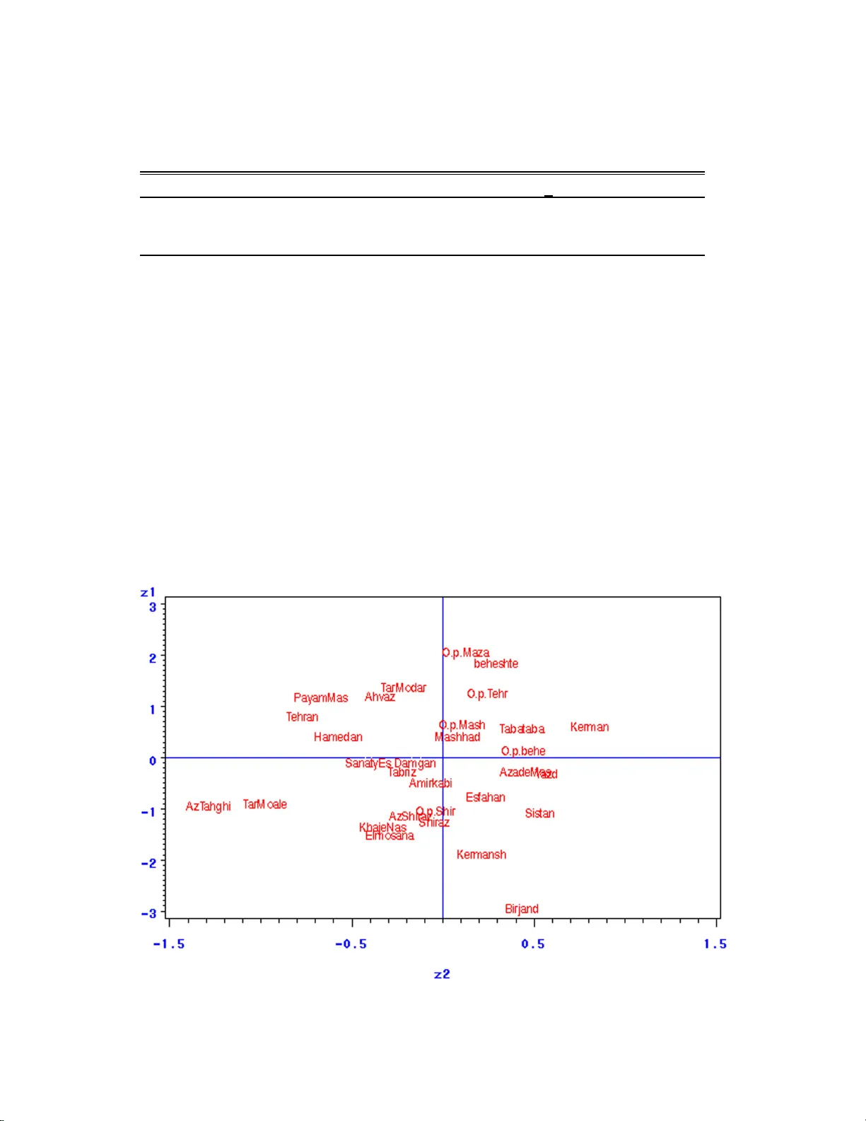
Bilinear Mixed Effects Mo dels F or Relations Bet w een Univ ersities S. Alimo radi and M. Khalil i an Jan uarey 2008 Abstract this article illustrates the use of linear a nd bilinear random effects mo dels to represent statistica l dep endencies that often c haracterize dyadic data such as in ternational relatio ns. In particular, w e sho w how to estimate mo dels for dy adic d ata th at simultaneously take into accoun t: r egressor v ariables and third-order dep endencies, such as transitivit y , clustering, and balance. W e app ly this n ew approac h to the relations among ph.d. of unive rsit y in Iran ov er the p erio d from 199 1-2005 , illustrating the p r esence and strength of second and thir d -order statistica l dep endencies i n these dat a. 1 In tro d u ction So cial netw ork data typic ally consist of a set of n actor s and a relational tie y i,j , measured o n eac h o r dered pair of actors i, j = 1 , . . . , n . This framew or k has man y applications in the so cial and b eha vioral scienc es including, for example, the b ehavior o f epidemics, the interconne ctedness of the W orld Wide W eb, and telephone calling patterns. In the simplest cases, y i,j is a dic ho t o mous v ariable indicating the presence or absence of some relation of intere st, suc h as fr iendship, colla b oration, transmission of information or disease, and so forth. The data are often represen ted by an n × n so ciomatrix Y . In the case of binary relations, the data can also b e though t of as a graph in whic h the no des are actors and the edge set is { ( i, j ) : y i,j = 1 } .So cial net work analysis is a broad a r ea of so cial scienc e researc h that has b een dev elop ed to describ e the relationships among interdependen t units (Holland and Leinhardt 1971, Bondy and Murty 1976). It is somewhat surprising t hat to date there a re no published applications using a so cial netw ork framework to study in ternational relations since it is eviden t at first blush that in t ernational p olitics is ab out the inte rdep endencies that app ear around the world. This is p erhaps due to the fact that most to ols for so cial net w ork analysis are fo cused on the simple case of binary (0-1) relations, where the data can b e represen ted by a simple graph (see W asserman a nd F aust 1 9 94, W asserman and P attison 19 96). D ealing with no n- binary data (suc h as counts o r contin uous data) or regressor v a riables has not been w ell addressed in the so cial net w orks literature (see Hoff, Ra ftery , and Handco c k 2002 f or a discussion). Herein, w e dev elop a generalized regression framew ork fo r a nalyzing and accoun ting for the dependencies in v alued and binary dy adic in ternat io nal relations data. This approac h builds on the so cial relations mo del (W arner, Kenn y and Stoto 1979; W ong 1982) that sp ecifies random effects for the origina tor and recipien t o f a relation or a ction, as w ell as allowin g for within dy a d correlation of relatio ns. W e expand up on previous approac hes b y allow ing for certain kinds of third- order dep endence using a n inner pro duct of laten t, unobserv ed c haracteristic v ectors. The use of inner pro ducts to mo del dep endencies is new, and related to the the recen t dev elopmen t of ”latent space” mo dels for dy adic data (Hoff, Raf tery and Handco ck 2002). 1 2 Laten t Space Appro ac hes to So cial Net w ork Analysis In some so cial net w ork data, the probabilit y of a relationa l tie b et w een t w o individuals may incre ase as the c haracteristics of the individuals b ecome more similar. A subset of individuals in the p opulation with a large num b er of so cial ties b etw een them ma y b e indicative of a group of individuals who hav e nearb y p ositions in this space of c har a cteristics, or ”so cial space”. V arious concepts of so cial space ha v e b een discussed b y McF arland and Brown (1973) and F aust (1988). In the contex t of t his art icle, so cial space refers to a space of unobserv ed latent c haracteristics that represen t p otential transitiv e tendencies in net w o r k relations. A probability measure o v er these unobserv ed c har acteristics induces a mo del in whic h the presenc e o f a tie b etw een tw o individuals is dep endent on the presence of o ther ties. Relations mo deled as suc h are probabilistically transitiv e in nature. The observ ation of i → j and j → k suggests that i and k a r e not to o f a r apart in so cial space, and therefore are more lik ely to ha ve a tie ( Holland and Leinhardt 197 1 ). In la ten t v a r iable mo del it is assumed each acto r i has an unkno wn p o sition z i in so cial space. The ties in the net w ork are assumed to b e conditionally indep enden t giv en these p ositions, and the pro babilit y of a sp ecific tie b etw een tw o individuals is mo deled as some f unction of their p ositions, suc h a s the distance b etw een the tw o actors in so cial space. Estimation of p ositions is simplified by the use o f a logistic r egr ession mo del, and confidence regions for la t en t p ositions are computable using standard MCMC algorit hms. 2.1 Distance Mo d els W e ta k e a conditio na l indep endence approach to mo deling by assuming that the presence or absence of a tie betw een tw o individuals is indep enden t of all other ties in the system, giv en the unobserv ed p ositions in so cial space of the t w o individuals, p ( Y | Z , X , θ ) = Y i 6 = j p ( y i,j | z i , z j , x i,j , α, β ) where X and x i,j are observ ed characteristics whic h are p oten tially pair - sp ecific and vec tor-v alued and α, β a nd Z are pa r a meters and p ositions t o b e estimated. A con v enien t pa rameterization is the logistic regression mo del in whic h the probability of a tie dep ends on the Euclidean distance b etw een z i and z j , as w ell as on observ ed cov ariat es that x i,j measure c haracteristics of the dy ad, η i,j = log p ( y i,j = 1 | z i , z j , x i,j , α, β ) p ( y i,j = 0 | z i , z j , x i,j , α, β ) = α + β ′ x i,j − | z i − z j | (1) 3 Linear Mixed Effects Mo dels for Exc hang e able Dy adic Data Supp ose w e a r e o nly inte rested in estimating the linear relationships b etw een resp onses y i,j and a p ossibly v ector v alued set of v ariables x i,j , whic h could include characteristics of unit i , characteristics of unit j , or c haracteristics sp ecific to the pair. In this case w e migh t consider the regression mo del y i,j = β ′ x i,j + ε i,j (2) where y i,i is t ypically not defined. It is of ten assumed in regression problems that the regressors x i,j con t a in enough information so that the distribution of the errors is inv ariant under p erm uta tions 2 of the unit lab els. This assumption is equiv alen t to the n × n matrix o f errors (with an undefined diagonal) having a distribution that is in v arian t under iden tical ro w and column p ermutations, so that { ε i,j : i 6 = j } is equal in distribution to { ε π ( i ) ,π ( j ) : i 6 = j } for any p ermutation π of { 1 , · · · , n } . This condition is called w eak row-and- column exc hangeability of an array . F or undirected dat a , suc h exc hangeability implies a ”random effects” represen tation of the errors, in that ε i,j ∼ f ( µ, a i , a j , γ i,j ) (3) where µ, a i , a j , γ i,j are indep enden t random v aria bles and f is a function to be sp ecified ( Aldo us 1985, Theorem 1 4 .11). If in addition to the ab ov e in v aria nce assumption w e a lso mo del the erro r s as Gaussian, then the join t distribution can b e represen ted in terms of a linear random effects mo del. In the more general case o f directed observ ations, w e can represen t the j oin t distribution of the errors as follows : ε i,j = a i + a j + γ i,j (4) where a 1 , . . . , a n i.i.d ∼ N (0 , σ 2 a ) ( γ i,j , γ j,i ) ′ ∼ M V N ( 0 , Σ γ ) , Σ γ = σ 2 γ σ 2 γ σ 2 γ σ 2 γ ! with effects otherwise b eing indep enden t. The co v ariance structure of the errors (and th us the observ ations) is as follo ws: E ( ε 2 i,j ) = σ 2 a + σ 2 b + σ 2 γ , E ( ε i,j ε i,k ) = σ 2 a E ( ε i,j ε j,i ) = ρ σ 2 γ + 2 σ ab , E ( ε i,j ε k ,j ) = σ 2 b E ( ε i,j ε k ,l ) = 0 , E ( ε i,j ε k ,i ) = σ ab T o analyze resp onses in pa r ticular sample spaces, the error structure described ab ov e can b e added to a linear predictor in a generalized linear mo del: θ i,j = β ′ x i,j + a i + b j + γ i,j , E ( y i,j | θ i,j ) = g ( θ i,j ) This is a generalized linear mixed-effects mo del with in v erse-link function g ( θ ), in whic h the obser- v ations are mo deled as conditionally indep enden t giv en the random effects, but are unconditionally dep enden t. 3.1 Mo d eling Third Order Dep endence P atterns Some dep endence patterns commonly seen in dydaic datasets ha ve b een given t he descriptiv e titles of bala nce and clusterabilit y . for example after fitting a regression mo del and obtaining the residuals { ˆ ξ i,j : i 6 = j } , the theoretic definitions of these concepts are as fo llo ws: Definition 3.1 F or s igne d r esiduals, a triad i, j, k is said to b e b alanc e d if ˆ ξ i,j × ˆ ξ j,k × ˆ ξ i,k > 0 Definition 3.2 Cluster ability is a r elaxation of the c onc ept of b alanc e. A triad is cluster able if it is b alanc e d or the r elations ar e al l ne gative. The ide a is that a cluster able triad c an b e divide d into gr oups wher e the me asur ements ar e p ositive within gr o ups a nd ne gative b etwe en gr oups. 3 Clusterabilit y and balanced cycle of residuals are sho wn g araphically in Figure 1. F ig u r e 1 : B al ance and C l us ter ability of C y cl es Hoff et al. (2002) used simple functions of laten t c ha r a cteristic v ectors in a fixed effects setting to capture some forms of t balance and clusterabilit y . F or example, they considered mo dels in whic h θ i,j = β ′ x i,j + f ( z i , z j ) where f ( z i , z j ) = | z i − z j | . w e consider a similar approach using the inner pro duct k ernel f ( z i , z j ) = z ′ i z j and giv e r andom a nd fixed effects interpretations. Adding the bilinear effect to the linear random effects in mo dels (4 ) giv es ε i,j = a i + a j + γ i,j + ξ i,j , ξ i,j = z ′ i z j (5) to suggest z 1 , . . . , z n i.i.d ∼ M V N ( 0 , σ 2 z I K × K ) the nonzero second and third order momen ts are E ( ε 2 i,j ) = 2 σ 2 a + σ 2 γ + k σ 4 z , E ( ε i,j ε i,k ) = σ 2 a E ( ε i,j ε j,i ) = σ 2 γ + 2 σ 2 a + k σ 4 z , E ( ε i,j ε k ,j ) = σ 2 a E ( ε i,j ε j,k ε k ,i ) = k σ 6 z , E ( ε i,j ε k ,i ) = σ 2 a Th us the effect ξ i,j = z ′ i z j can b e in terpreted as a mean-zero random effect able to induce a par ticular form of third-o rder dep endence often found in dy adic datasets. 4 Bilinear Mixed Effects Mo dels P arameters Estimation T o obtain a ”cleaner” partition of the v ariance and a more efficien t MCMC sampling sc heme,in mo del (2) w e decomp ose x i,j in t o x i,j = ( x i,j , x s ,i , x s ,j ) i.e. into dyad sp ecific regressors x i,j , sender sp ecific regressors x s ,i and receiv er sp ecific regressors x s ,j . The generalized bilinear mo del is then rewritten as θ i,j = β d x i,j + β ′ s x s ,i + β ′ s x s ,j + ε i,j or equiv alen tly θ i,j = β d x i,j + s i + s j + γ i,j + z ′ i z j (6) s i = β ′ s x s ,i + a i where x s ,i = (0 / 5 , x i ) ′ and β s = ( β 0 , β s ) ′ . This parameterization for the linear unit-lev el effects is similar t o the ”cen tered” pa r a meterizations suggested by Gelfand et al. (1995, 1996). Note that an in t ercept can b e thought of as b oth a sender or receiv er sp ecific effect. F or symmetry , we include the constan t 1 / 2 at the b eginning of eac h x s ,i and x s ,j v ector. Using the ab ov e reparameterization for θ i,j , w e estimate the parameters for the generalized bilinear 4 regression mo del b y constructing a Mark o v c hain in { β d , β s , σ 2 a , σ 2 z , Σ γ , Z } (where Z denotes the k × n matrix of lat ent v ectors),ha ving p ( β d , β s , σ 2 a , σ 2 z , Σ γ , Z ) as the inv ariant distribution. This is obtained via an algorithm based o n Gibbs sampling, whic h a lso samples s,r and the θ ’s. The basic alg orithm is to iterate the follow ing steps: 1. Sample linear effeects: (a) Sample β d , s | β s , σ 2 a , σ 2 z , Σ γ , θ , Z (linear regression); (b) Sample β s | s , σ 2 a (linear regression); (c) Sample σ 2 a and Σ γ from their full conditionals. 2. Sample bilinear effects: (a) F or i = 1 , . . . , n sample z i |{ z j , j 6 = i } , θ , β , s , σ 2 z , Σ γ (a linear regression); (b) Sample σ 2 z from its full conditional. 3. Sample dyad sp ecific parameters: Up date ( θ i,j , θ j,i ) using a Metrop olis-Hastings step: (a) Prop ose  θ ∗ i,j θ ∗ j,i  ∼ MVN   β ′ x i,j + a i + a j + z ′ i z j β ′ x j,i + a j + a i + z ′ j z i  , Σ γ  (b)Accept  θ ∗ i,j θ ∗ j,i  with probability α = min  P ( y i,j | θ ∗ i,j ) P ( y j,i | θ ∗ j,i ) P ( y i,j | θ i,j ) P ( y j,i | θ j,i ) , 1  for more detail see Metrop olis et al.(19 5 3) and Hastings et al. (1970). V arious combinations of the ab ov e steps can b e used to estimate differen t mo dels. T he steps in 1 alo ne provide a Bay esian estimation pro cedure fo r the linear regression problem having an error cov ariance as in (2). Ba y esian estimation o f the normal bilinear mo del with the iden tity link could pro ceed b y replacing each θ i,j with y i,j and only iterating steps 1 and 2 . Estimation of a generalized linear mixed effects mo del with random effects structure giv en by (2) could pro ceed by itera t ing steps 1 and 3 . The full conditional distributions required to p erform steps 1 and 2 are giv en b elow. 4.1 Conditional Distributions for the Linear Effects Comp onen ts Similar to W o ng’s (1982 ) approa c h to the in v ariant normal mo del, w e let u i,j = θ i,j + θ j,i − 2 z ′ i z j v i,j = θ i,j − θ j,i f or i < j W e then hav e u i,j = β d ( x i,j + x j,i ) + 2( s i + s j ) + δ u i,j , δ u i,j = γ i,j + γ j,i v i,j = 0 with definition u = { u i,j } , δ u = { δ u i,j } and X u the appropriate design matrices: u = X u  β d s  + δ u (7) and u ∼ M V N ( X u Φ , σ 2 u I M ) , σ 2 u = 4 σ 2 γ (8) 5 where M = n ( n − 1) 2 and Φ = ( β d s ′ ) ′ . w e hav e s ∼ M V N ( X s β s , σ 2 a I n × n ) (9) and X s = ( x s , 1 , x s , 2 , . . . , x s ,n ) ′ . The full conditional distribution of mo del (6) is then L ( u | β d , s , σ 2 γ ) × L ( s | β s , σ 2 a ) ∝ exp  − 1 2 h ( u − X u Φ ) ′ ( u − X u Φ ) /σ 2 u  × exp  − 1 2 h ( s ′ s + β ′ s X ′ s X s β s − 2 β ′ s X ′ s s ) /σ 2 a i  (10) join t p osterior distributions using a ppro ac h Bay esian is then prop ortional to pro duct of prior densit y and function lik eliho o d (gelman 2003): π ( s , β d , β s , σ 2 a , σ 2 γ | u ) ∝ L ( u | β d , s , σ 2 γ ) L ( s | β s , σ 2 a ) π ( β d ) π ( β s ) π ( σ 2 a ) π ( σ 2 γ ) (11) note that we assume the parameters is indep enden t. • F ull conditi onal of ( β d , s ) The full conditional distribution of ( β d , s ) is then prop ortional to join t p o sterior densit y and obtain with omitting the terms that uncondition to ( β d , s ). π ( β d , s | β s , σ 2 a , σ 2 γ , u ) ∝ L ( u | β d , s , σ 2 γ ) L ( s | β s , σ 2 a ) π ( β d ) F or a m ultiv aria t e normal ( µ β d , σ 2 β d ) prior distribution on β d and then with o mitt ing the terms that uncondition to ( β d , s ): π ( β d , s | β s , σ 2 a , σ 2 γ , u ) ∝ exp ( Φ ′ "  µ β d /σ 2 β d X s β s /σ 2 a  + X ′ u u /σ 2 u # − 1 2 Φ ′ "  σ − 2 β d 0 0 σ − 2 a I n × n  + X ′ u X u /σ 2 u # Φ ) The conditional distribution is thus β d , s | β s , σ 2 a , σ 2 γ , u ∼ M V N ( µ, Σ ) where µ = Σ "  µ β d /σ 2 β d X s β s /σ 2 a  + X ′ u u /σ 2 u # and Σ = "  σ − 2 β d 0 0 σ − 2 a I n × n  + X ′ u X u /σ 2 u # − 1 6 • F ull conditi onal of β s The full conditional distribution o f β s is then prop ortional to j oin t p osterior densit y and obtain with omitting the terms that uncondition to β s . using ( 1 1) π ( β s | s , σ 2 a , u ) ∝ L ( s | β s , σ 2 a ) π ( β s ) F or a m ultiv ar ia te normal on β s as follows β s ∼ M V N  µ β s , Σ β s  and then with omitting the terms that uncondition to β s . β s | s , σ 2 a , u ∼ M V N ( µ , Σ ) where µ = Σ h Σ − 1 β s µ β s + X ′ s s /σ 2 a i , Σ =  Σ − 1 β sr + X ′ s X s /σ 2 a  − 1 • F ull conditi onal of σ 2 a The full conditional distribution of σ 2 a is then prop ortional to joint p osterior densit y and obtain with omitting the terms that uncondition to σ 2 a . π ( σ 2 a | a ) ∝ L ( a | σ 2 a ) π ( σ 2 a ) note that a 1 , . . . , a n i.i.d ∼ N (0 , σ 2 a ) L ( a | σ 2 a ) ∝ | σ 2 a | − n 2 exp  − 1 2 n X i =1 a 2 i /σ 2 a  F or a in ve rse g a mma distribution on σ 2 a as follo ws σ 2 a ∼ I G ( α a 1 , α a 2 ) The full conditional distribution of σ 2 a is then σ 2 a | a ∼ I G  α a 1 + 1 2 n , α a 2 + n X i =1 a 2 i /σ 2 a  • F ull conditi onal of σ 2 γ note that σ 2 γ = σ 2 u / 4 to find The full conditional distribution of σ 2 u using (1 1) π ( σ 2 u | β d , s , σ 2 γ , u ) ∝ L ( u | β d , s , σ 2 γ ) π ( σ 2 u ) F or a in v erse gamma distribution on σ 2 u as f ollo ws σ 2 u ∼ I G ( α u 1 , α u 2 ) and with o mitt ing the terms that uncondition to σ 2 u .The full conditional distribution of σ 2 u is then σ 2 u | β d , s , σ 2 γ , u ∼ I G  α u 1 + 1 2 M , α u 2 + ( u − X u Φ ) ′ ( u − X u Φ )  4.2 Conditional distributions for the Bilinear Effects Comp onen t Let e i,j = ( θ i,j + θ j,i − ˆ u i,j ) / 2, the residual of the symmetric part of the matrix of θ ’s after fitting the linear effects, and let δ u ,i,j = γ i,j + γ j,i . Considering the full conditiona l of z i , w e hav e e i, 1 = z ′ i z 1 + δ u ,i, 1 / 2 e i, 2 = z ′ i z 2 + δ u ,i, 2 / 2 . . . e i,n = z ′ i z n + δ u ,i,n / 2 (12) 7 can write the equations to fa ce matrix: e i, − i = Z ′ − i z i + 1 2 δ i, − i (13) where e i, − i errors vector to face { e i,j : i 6 = j } and Z − i matrix k × ( n − 1) obtain to omit of i column Z . for example for i = 1: e 1 , − 1 =       e 1 , 2 e 1 , 3 . . . e 1 ,n       , Z − 1 =       z ′ 2 z ′ 3 . . . z ′ n       ′ note that V ar ( δ u ,i,j / 2) = σ 2 u / 4 lik eliho o d function mo del (13)is then: L ( e i, − i | Z − i , z i , σ 2 u ) ∝ exp ( − 1 2 h 4( e i, − i − Z ′ − i z i ) ′ ( e i, − i − Z ′ − i z i ) /σ 2 u i ) p osterior distributions z i is prop ortiona l to pro duct of prior densit y and function likelihoo d. to assume z i ∼ M V N ( 0 , Σ z ) π ( z i | Z − i , σ 2 u , Σ z ) ∝ L ( e i, − i | Z − i , z i , σ 2 u ) π ( z i ) • F ull conditi onal of z i The full conditional distribution of z i is then prop ortiona l to joint p osterior densit y and o btain with omitting the terms that uncondition to z i . π ( z i | Z − i , σ 2 u , Σ z ) ∝ exp ( − 1 2 × 4  h z ′ i Z − i Z ′ − i z i /σ 2 u i − h 2 z ′ i Z − i e i, − i /σ 2 u i  ) × exp ( − 1 2 h ( z ′ i Σ − 1 z z i ) i ) for other hands π ( z i | Z − i , σ 2 u , Σ z ) ∝ exp ( z ′ i h 4 Z − i e i, − i /σ 2 u i − 1 2 z ′ i h Σ − 1 z + 4 Z − i Z ′ − i /σ 2 u i z i ) the full conditional of z i is m ultiv ariate normal ( µ , Σ ) with µ = 4 ΣZ − i e i, − i /σ 2 u , Σ =  Σ − 1 z + 4 Z − i Z ′ − i /σ 2 u  − 1 4.3 Conditional distributions for the matrix co v ariance Σ z to assume z i ∼ M V N ( 0 , Σ z ) L ( z 1 , . . . , z n | Σ z ) ∝ | Σ z | − n 2 exp ( − 1 2 tr Σ − 1 z Z ′ Z ) p osterior distributions for Σ z is prop ortional to pro duct of prio r densit y and function likelihoo d. π ( Σ z | Z ) ∝ L ( z 1 , . . . , z n | Σ z ) π ( Σ z ) • F ull conditi onal of Σ z The full conditional distribution of Σ z is then prop ortional to jo in t p osterior densit y a nd obtain with 8 omitting the terms that uncondition to Σ z . to assume prior distributions, in ve rse wishart fo r Σ z as follo ws Σ z ∼ IW ( Σ z0 , ν ) w e ha ve π ( Σ z | Z ) ∝ | Σ z | − ( ν + n ) 2 exp ( − 1 2 tr Σ − 1 z  Σ z0 + Z ′ Z  ) to note tha t prop ert y of in v erse wishart,The full conditiona l distribution of Σ z is Σ z | Z ∼ I W  Σ z0 + Z ′ Z , ν + n  Alternativ ely , if w e restrict Σ z to b e σ 2 z I k × k and use an in v erse gamma fo r σ 2 z as follows σ 2 z ∼ I G ( α 0 , α 1 ) and with omitting the t erms that uncondition to σ 2 z π ( Σ z | Z ) ∝ σ 2 z − ( α 0 + nk/ 2+1) exp n − [ α 1 + tr Z ′ Z / 2] /σ 2 z o then σ 2 z | Z ∼ I G ( α 0 + nk / 2 , α 1 + tr Z ′ Z / 2) 4.4 Selecting the Laten t Dimension One issue in model fitting is the sele ction of the dimension k of the latent v ariables z . Selection of K could dep end on the go a l of the analysis. F o r example, if the goal is descriptiv e, i.e. the desired end result is a decompo sition of the v ariance into inte rpretable comp onen ts, then a c hoice of K = 1 , 2 or 3 w ould allo w for a simple graphical presen t a tion of a m ultiplicative comp onent of the v ariance.Alternativ ely , one could examine mo del fit as a function of K based on the log- lik eliho o d. ha ving obtaind p osterior estimates ˆ Ψ ( k ) = { ˆ β , ˆ a , ˆ b , ˆ Z , ˆ Σ γ } fo r a range of K , one can compare the v alue of lo g p ( Y | ˆ Ψ ( k ) ) to assess mo del fit v ersus complexit y . Az a funtion of K , the Ak aik e informa t io n criterion(AIC) and Bay esian information criterion (BIC) are AI C ( k ) = − 2 log p ( Y | ˆ Ψ ( k ) ) + c + [2 n ] × k and B I C ( k ) = − 2 log p ( Y | ˆ Ψ ( k ) ) + c + h n log  n 2 i × k where the suggestion is to prefer the mo del with a lo w est v alue of the criterion. f or hierarc hical mo del, Spiegelhalter, Best, Carlin, and v an der Linde (200 2) suggested usisng the deviance information criterion (DIC), D I C ( k ) = − 2 lo g p ( Y | ˆ Ψ ( k ) ) + 2 × p ( k ) D where the p enalt y p ( k ) D on the mo del complexit y is giv en b y p ( k ) D = − 2 × n E h log p ( Y | ˆ Ψ ( k ) ) | Y i − log p ( Y | ˆ Ψ ( k ) ) o this exp ection can b e approximated by av eraging ov er MCMC samples. the p enalty term p ( k ) D has b een referred to as the ”effectiv e n um b er o f parameters” b ecause it ha s this in terpretation in normal linear mo del. 9 5 Data Analysis: Rel ations Bet w e en Univ er s ities for fitting bilinear mixed effect mo del, w e a nalyze da t a on relations b et w een 30 univ ersit y in Ira n. W e tak e our resp onse y i,j to b e the total n umber of ”p ositive ” actions rep ortedly initiated b y unive rsit y i with target j fro m 1 991 to 2005 . Pos itiv e actions here include articles in connection statistics sciences that they hav e b een published in Iranian Statistical Conference b o ok. x i,j is the geographic distance b et w een univ ersity i and j and x i is log p opulatio n(n umber of master in univ ersit y). The o ccurrence of a action b etw een a ny t wo given coun tries in these data is rare, with 86of the nondiagonal en tries o f the so ciomatrix b eing equal to 0. some descriptiv e plo ys of the raw data a re g iven in Figure 2. P anel (a) plots the resp onse on a log scale v ersus the geogr a phic distance in thousands of kilometer b et w een univ ersity i and j . More precisely , this distance is t he minimum distance betw een tw o univ ersit y , whic h is 0 if i a nd j in one cit y . O n av erage, the n um b er o f action decreases as geographic distance in- creases. P anel (b) plot s log(1 + P j : j 6 = i y i,j ), versu s log p opula t ion , wic h suggests a p ositiv e relationship b et w een r esp o nse and p opulation. The quantities P j : j 6 = i y i,j is t ypically called the o utdegree of unit i . F ig u r e 2 : Rel ationships B etw een ( a ) R esponse and Geog r aphic D istance, and ( b ) O utdeg r ee and P opul ation ( a ) ( b ) 5.1 Evidence of Third-Order Dep endence Before fitting a somewhat complicated bilinear P oisson regression mo del, w e ev aluate the necessit y of suc h an effort b y lo oking for evidence of balance and clusterabilit y in the data. w e do this b y fitting a simple linear regression on the logtransformed data and examining the residuals for third- order dep endencies of the t yp es describ ed. more sp ecifically , w e obtain ordinary least squares estimates for the regression mo del log( y i,j + 1) = β 0 + β d x i,j + a i + a j + ξ i,j There are sev eral indicatio ns of third-order dep endence in these residuals: 1. Because the mean o f the residuals is 0, independence of the residuals implies that t he av erage v alue of the pro duct ˆ ξ i,j ˆ ξ j,k ˆ ξ k ,i o v er triads also should b e 0 ( the concept of indep endence of the residuals is E ( ˆ ξ i,j ˆ ξ j,k ˆ ξ k ,i ) = 0). As discussed in section 3.1, a v alue la rger than 0 would indicate some degree o f balance. The empirical a v erag e ov er triads turns out to b e 0 . 00 3 5. 2. The fraction of residuals that are po sitiv e is p = 0 . 4 5(the distribution of residuals is no t sym- metric). Under indep endence, the prop ortion of cycles that w e w ould exp ect in the tw o balanced 10 categories sho wn in Figure 1 (+++ and +–) are p 3 = 0 . 09 1 and 3 p (1 − p ) 2 = 0 . 4, whereas the observ ed prop ortion are 0 . 115 and 0 . 38 5 . The observ ed prop ortio n in the unclusterable category (++-) is 0 . 333 and the v alue exp ected under indep endence is 3 p 2 (1 − p ) = 0 . 3 34. The exp ected prop ortio n in the clusterable but unbalance category is 0 . 166, and the observ ed prop ortion is 0 . 167. 3. As describ ed in section 3.1, in a balance system w e exp ect that if ˆ ξ i,j > 0, then ˆ ξ j,k and ˆ ξ i,k will ha v e the same sign. suc h a pattern is sho wn g r aphically in F ig ure 3, whic h for each pair { i, j } plots ˆ ξ i,j v ersus the prop o rtion of other no des k for whic h ˆ ξ i,k × ˆ ξ j,k > 0. Altho ug h the distribution of residuals is far fro m normal, we do see some indication of this ty p e of t hird- order dep endence. As w e w ould expect f rom a balanced system, pair s { i, j } for whic h ˆ ξ i,j is less than 0 generally ha v e dissimilar residuals to other, ˆ P ( ˆ ξ i,k × ˆ ξ j,k > 0) tends to b e 0 . 47, pa ir { i, j } for whic h ˆ ξ i,j is gr eat er than 0 generally hav e similar residuals to other, ˆ P ( ˆ ξ i,k × ˆ ξ j,k > 0)tends to b e greater t ha n 0 . 52. in the next section w e analysis results of fitting bilinear mixed mo del. F ig u r e 3 : B al anced Residu als 5.2 Mo d el Selection W e fit the bilinear mixed effects mo del to the data using a P oisson distribution and the log-link, so that eac h resp onse y i,j is assumed to hav e come from a Poisson distribution with mean exp ( θ i,j ) , and that t he y ’s are conditionally indep enden t giv en the θ ’s. assume follo wing mo del: θ i,j = β d x i,j + β ′ s x s ,i + β ′ s x s ,j + ε i,j where x s ,i = (0 / 5 , x i ) ′ and β s = ( β 0 , β s ) ′ . T able 1 includes are t he the marginal probabilit y criteria, the D IC p enalt y , p D , in the third column, the AIC criterion , the BIC criterion and the DIC crite- rion. In t erms o f t he marginal lik eliho o d criterion, the biggest impro v ements in fit a r e in going from K = 1 to K = 2 and from K = 2 to K = 3. Using the AIC criterion and p enalizing the impro v emen t in lik eliho o d by the num b er of additional parameters, w e w ould ch o ose K = 0. The BIC, with a higher p enalty on the n um b er of parameters, fa v o rs K = 0 . In con trast, the DIC fav ors K = 1. 11 Note that the increase in the DIC p enalt y tends to decrease the DIC. But note that for mo dels whit K = 1 and K = 2 the D IC criterion hav e lik e predictiv e a bility , then based on these results and o ur abilit y to plot in t w o dimensions, w e choose to presen t the a nalysis of the K = 2 mo del in more detail. K log p ( Y | ˆ β , ˆ s , ˆ Z , ˆ σ 2 γ ) P D AI C ( K ) B I C ( K ) D I C ( K ) 0 − 167 . 30 − 6 . 00 334 . 6 334 . 6 322 . 62 1 − 178 . 82 − 29 . 28 417 . 6 436 . 79 299 . 08 2 − 169 . 30 − 9 . 49 458 . 6 496 . 9 319 . 80 3 − 152 . 96 21 . 66 485 . 8 543 . 3 349 . 24 4 − 157 . 03 12 . 62 554 . 0 630 . 6 339 . 30 T able 1 : E v al uation of K One Mark ov c hains of length 100,000 w as constructed using t he a lgorithm describ ed in section 4. The second chain used starting v a lues obtained fro m the f o llo wing pro cedure: • fitting generalized linear mo del,using geographic distance as a regressor and sender and receiv er lab els as factor v ariables. log( y i,j + 1) = β d x i,j + a i + a j + ξ i,j w e let parameters of prior distribution for β d to case v ar ( ˆ β d ) = σ 2 β d and µ β d = ˆ β d • letting ˆ s i = ( ˆ a i + ˆ a j ) / 2 and fitting ordinary regression mo del w e hav e ˆ s i = β ′ s x s ,i + a i w e let Σ β s = cov ( ˆ β s ), µ β s = ˆ β s and ( α a 1 , α a 2 ) = (2 , ˆ σ 2 a ) • The itera t iv ely rew eigh ted least-squares fitting pro cedure pro duces a matrix R of working residuals, with the of dia g onal elemen ts undefined. An estimate ˆ Z of Z w as then obtained b y a ppro ximating R with a matrix pro duct of the fo rm Z ′ Z . This can b e done with a n iterativ e least-squares pro cedure, similar to t he Gibbs sampling pro cedure outlined in Section 4 : see ten Berge and Kiers (1989) for more details o n this problem. • An estimate o f Σ γ is then obtained from E = R − ˆ Z ′ ˆ Z . w e define ˆ σ 2 u = v ar ( E + E ′ ) then ˆ σ 2 γ up date fro m ˆ σ 2 u . F ig u r e 4 : M ar g inal M C M C outpu t f or par ameter s β d and β 0 Samples of pa r a meter v alues were sa ved from the Mark o v c hains ev ery 100 iteratio ns, and for example for β d and β 0 are plotted in Figures 4. The c hain app ear to hav e achiev ed stationarit y aft er ab out 10,0 00 iterations, a nd so w e ba se our inference o n the sa v ed samples after this p oint. P o sterior means and standard deviations of the mo del parameters, based on the sa ved MCMC samples are giv en in T able 2. 12 As in the raw data, w e see a negativ e relation b et w een respo nse and geog r a phic distance E [ β d | Y ] = − 2 . 38, and a p ositiv e relatio n b et w een resp onse and log n um b er of master in univ ersit y ( E [ β s | Y ] = 0 . 65). β d β 0 β s σ 2 a σ 2 γ σ 2 z 1 σ 2 z 2 M E AN − 2 . 38 − 3 . 4 1 0 . 65 1 . 1 0 . 86 0 . 64 0 . 52 S D 0 . 38 0 . 98 0 . 2 9 0 . 41 0 . 48 0 . 32 0 . 31 T able 2 : P oster ior means and standar d dev iations f or k = 2 Next, w e analyze the p osterior distribution of the the k × n matrix o f la ten t v ectors Z . In F igure 5 has ploted sample z ’s ov er the plot of the means. G enerally , t w o univ ersit y will b e mo deled as ha ving z in the same direction if they ha v e large resp onses to one another r elat ive to their total n umber of actions and co v ariate v alues, and/or if their r esp o nses in volving other univ ersit y are sim- ilar. F or example, 3 univ ersit y Shiraz, Olum p ezeshky Shiraz a nd Azad Shira z ha v e placed in the same direction and so these univ ersit y are similar b ecause they had minim um 3 partner article, a lso Olum p ezeshky Shiraz and Azad Shiraz did not ha v e connection with other univ ersit y exept Shira z. Mashhad univ ersit y ha d con t a cted at least with 12 univ ersit y , th us it had rep osed in cen tral of plot. univ ersity T arbiat Mo dares in addition to connections with other unive rsit y , it had 1 1 partner art icle with Azad Olo um T ahghighat so this t w o univ ersit y hav e placed in the same direction. F ig u r e 5 : P oster ior mean of Z 13 References [1] Aldous,D.J.(1985),Exc hangeabilit y and related topics, in Ecole dete de probabilites de Sain t- Flour, XI I I-1983 , v ol. 11 17 of Lecture Notes in Math., pp. 1-19 8, Springer, Berlin. [2] Bondy A., Murty U.S.R.(1976), Graph Theory with Applications, North Holland, New Y ork. [3] F aust K.(1988) , Comparison of Metho ds for P ositional Analysis: Structural and General Equiv- alence, So cial Net w orks, 10 :313 - 341. [4] Gelfand A.E., Sah u S.K., Carlin B.P . (1995), Efficien t parameterisations for normal linear mixed mo dels, Biometrik a 82 479-4 8 8. [5] Gelfand A.E., Sah u S.K., Carlin B.P .(1996),Efficien t parametrizatio ns for generalized linear mixed mo dels, in Bay esian statistics 5 , eds.J. Bernardo et al., New Y o rk: Oxford Univ. Press, pp 165- 180. [6] Gelman A., Carlin J.B., Stern H.S., Rubin D.B.(2003), Bay esian data a nalysis, 2nd Edition, Chapman a nd Ha ll, London. [7] Hastings W. K.(19 70), Mon te Carlo sampling Metho ds using Mark o v Chains and their Appli- cations, Bio metrik a 57 : 97- 109. [8] Hoff P .D., Ra ftery A.E., Handco ck M.S.(20 02), Laten t space approaches to so cial net work anal- ysis, Journal of the American Statistical Asso ciation, 97 1090- 1 098. [9] Hoff P .D .( 2005), Bilinear Mixed Effects Mo dels for D y adic Da ta, , Journa l of the American Statistical Asso ciation, 100 N0.4 69: 286-295. [10] Holland P .W., Leinhardt S.( 1971). T ransitivit y in structural mo dels of small groups. Compar- ativ e Gro up Studies 2 : 107 -124. [11] McF arland D ., Brown D.(1973), So cial Distance as Metric: A Systematic In tro duction to Small- est Space Analysis, in Bonds of Pluralism: The F orm and Substance of Urban So cial Net works , ed. E. Laumann, New Y ork: Wiley , pp. 21 3 -253. [12] Metrop olis N., Rosen bluth A.W., Rosen bluth M.N., T eller A.H., T eller E. (1953) , Equations of state calculations b y fast computing ma chines , Journal o f Chemical Phy sics, 21 :1087-1091. [13] Spiegelhalter D.J. , Best N.G , Carlin B.P , v an der Linde A.(20 02), Bay esian Measures of Mo del Complexit y and Fit, Journal of the R o y al Sta tistical So ciet y . Series B (Statistical Metho dology), 64 , No.4: 5 8 3-639. [14] W arner R., Kenn y D.A., Stoto M.(1979), A new r ound r obin analysis of v ariance fo r so cial in t eraction data, Journal of P ersonality and So cial Psyc hology 37:1742- 1757. [15] W asserman S., F aust K.(1 994), So cial Net w ork Analysis, Cam bridg e Unive rsit y Press. [16] W asserman S., P attison P .(1996), Logit mo dels and logistic regressions for so cial net w orks:I. An in t ro duction to Mark o v random g r aphs and p ∗ , Psyc hometrik a 61 : 401-426. [17] W ong G.Y.(1982), Round Robin Analysis of V ariance via Maxim um Like liho o d, Jo ur na l of the American Statistical Associat io n 77 : 714-724. 14