Imprecise probability trees: Bridging two theories of imprecise probability

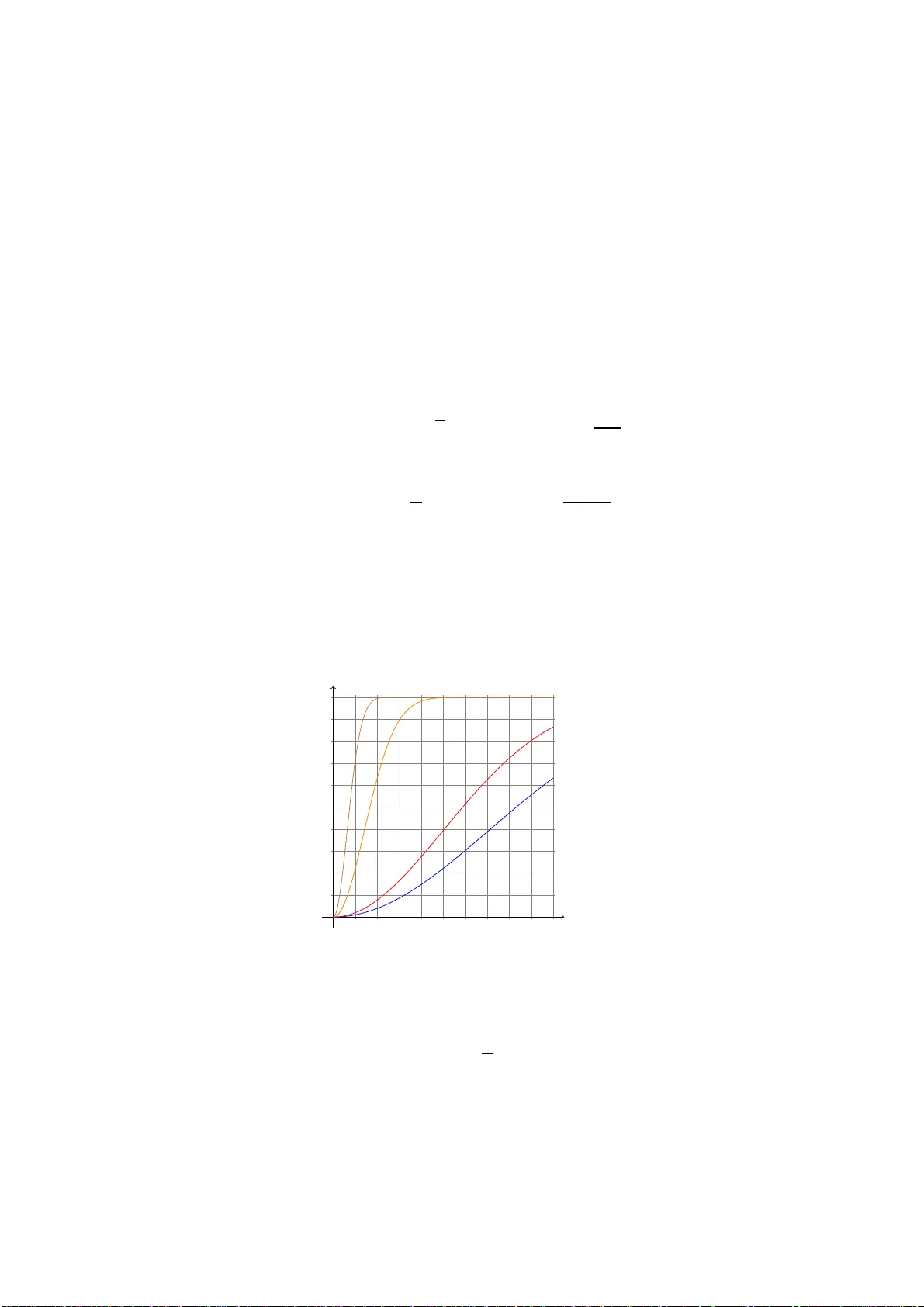
IMPRECISE PROB ABILITY TREES: BRIDGING TWO THEORIES OF IMPRECISE PROB ABILITY GER T DE COOMAN AND FILIP HERMANS A B S T R AC T . W e gi ve an ov ervie w of tw o approa ches to pro bability theory where lo wer and upper probabili ties, rather than probabili ties, are used: W alle y’ s be havioural theory of imprecise probabilit ies, and Shafer and V ovk’ s game -theoretic acco unt of pro bability . W e sho w that the two theories are more closel y related than would be suspected at ﬁrst sigh t, and we est ablish a correspondence bet ween them that (i) has an intere sting interpret ation, and (ii) allo ws us to freely import results from one th eory into the other . Our approach leads to an accou nt of pr obability trees and random processes in the frame work of W alley ’ s theory . W e indica te how our results ca n be used to red uce the comput ational complexi ty of deali ng with impre cision in proba bility trees, and we pro ve a n inter esting and qui te genera l versi on of the weak l aw of large numbers. 1. I N T RO D U C T I O N In recent years, we h a ve witnessed the growth of a numb er of theories of uncer tainty , where imprecise (lower and upper) probabilities and previsions, rather than precise (o r point-valued) pr obabilities and previsions, h a ve a central part. Here we consider tw o of them, Glenn Shaf er an d Vladimir V ovk’ s ga me-theoretic acco unt o f prob ability [30], which is intr oduced in Sectio n 2 , and Peter W alley’ s behavioural theory [34], outlin ed in Section 3. These seem to have a ra ther different interp retation, and they certain ly ha ve been inﬂuenced by dif fer ent schools o f thou ght: W alley f ollo ws the tradition o f Frank Ramsey [22], Bruno de Finetti [1 1 ] and Peter W illiams [40] in trying to establish a rational mode l for a subject’ s belief s in terms of her beh a viour . Shafer and V ovk fo llo w an appr oach that has many other inﬂuences as well, and is strong ly colou red by ideas abou t gambling systems and ma rtingales. They use Cour not’ s Principle to interp ret lo wer and upper prob- abilities (see [29]; and [30, Chap ter 2] fo r a nice historical overvie w), wh ereas o n W alle y’ s approa ch, lower and up per pr obabilities are deﬁn ed in terms of a subject’ s betting rates. What we s et ou t to do here, 1 and in p articular in Sections 4 and 5, is to show that in many practical situations, the two approa ches ar e strongly connecte d. 2 This implies th at quite a few results, valid in one theory , can automatically be con verted and re interpreted in terms of the other . M oreover , we shall see that we can develop an account of coherent immediate prediction in the context of W alley’ s behavioural theory , and prove, in Section 6, a weak law of large nu mbers with an intuiti vely appealing interpretation. W e use this weak law in Section 7 to sugg est a way of scoring a predictive mod el th at satisﬁes A. Philip Dawid’ s Pr equen tial Principle [5, 6]. Why do we belie ve th ese results to be important, or even relev ant, to AI? Probabilistic models are intended to repr esent an agent’ s belief s about the world he is o perating in, and which describ e and ev en d etermine the ac tions he will take in a diversity of situation s . K ey wor ds and phrases. Game-theoreti c probabilit y , imprecise probabilit ies, coherence, conglomerabili ty , e vent tree, probabili ty tree, imprec ise probab ility tre e, lower pre vision, immediate prediction, Prequential Princi- ple, la w of lar ge numbers, Hoeffdi ng’ s ineq uality , Marko v cha in, random process. 1 An earl ier and condensed ve rsion of thi s paper , with much le ss discussion and wit hout proofs, was present ed at the ISIPT A ’07 confe rence [7]. 2 Our line of reasoning here should be contrasted with the one in [29], where Shafer et al. use the game- theoret ic frame work dev eloped in [30] to construct a theory of predicti ve upper and lo wer previ sions whose interpre tation is based on Cournot ’ s Princip le. See also the comments near the end of Sect ion 5. 1 2 GER T DE COOMAN AND FILIP HERMANS Probability theory pr o vid es a no rmati ve system for reasoning and mak ing decisions in the face o f uncertainty . Bayesian, or precise, probab ilit y m odels have the pr operty that they are co mpletely decisive: a Bayesian agent always has an op timal ch oice when faced with a number of altern ati ves, whatever h is state of info rmation. While many may view this as an advantage, it is not al ways very r ealisti c. Impre cis e probability mode ls try to d eal with this problem by e xp licitly allowing f or ind ecision, wh ile retainin g the normati ve, or coh erentist stance of the Bayesian app roach. W e refer to [8, 34, 35] for discussions about how this can be done. Imprecise prob ability mo dels ap pear in a nu mber of AI-related ﬁelds. For in s tanc e in pr o babilistic logic : it w as already known to George Boole [1] th at the result of probab ilis tic inference s m ay be a set o f pro babilities (an imp recise proba bility m odel), r ather than a single prob ability . This is also imp ortant for dealing with missing o r incom plete data, leading to so-called partial iden tiﬁ cation of pro babilities, s ee f or instance [9, 19]. T here is also a growing literatur e o n so-called cr edal nets [3, 4]: these are essentially Bayesian nets with imprecise condition al p robabilities. W e are con vin ced that it is main ly the mathematical and com putational complexity often associated with imprecise p robability models that is keeping the m from becom ing a more widely used tool for m odelling uncertainty . But we believe that the results repo rted h ere can h elp m ak e inroads in reduc ing this complexity . Ind eed, the upsho t of our being able to connec t W alley’ s approa ch with Shaf er and V ovk’ s, is tw ofo ld. First of all, we c an develop a theor y of impr ec is e pr oba bility trees : proba bility trees where the transition fr om a n ode to its children is described b y an imp recise pr obability mod el in W alley’ s sense. Our re s ults provide th e nec ess ary apparatus for making in ferences in such trees. And because probability trees are so closely related to ra ndom processes, this effectively brin gs us in to a po sit ion to start developing a theor y of (ev en t-dri ven) random pr ocesses where the uncertainty can be described using imprecise pr obability models. W e illustrate this in Examples 1 and 3, and in Section 8. Secondly , we are able to prove so-called Marginal Extension results (Th eorems 3 and 7, Proposition 9) , which lead to backwards recu rsion, and dynam ic pr ogramming-like meth- ods that allow for an expone ntial red uction in the com putational comp le xity o f making inference s in such imprec is e pr obability trees. This is also illustra ted in Exam ples 3 and Section 8. For (precise) pr obability tre es , similar tech niques were described in Shafer ’ s book o n causal reason ing [2 7 ]. They seem to go b ack to Christiaan Huyg ens, who dr e w the ﬁrst prob ability tree , and showed how to reason with it, in his solutio n to Pascal an d Fermat’ s Problem of Points. 3 2. S H A F E R A N D V OV K ’ S G A M E - T H E O R E T I C A P P RO AC H T O P RO B A B I L I T Y In their game-theo retic appr oach to prob ability [30], Shafer a nd V ovk consider a game with two players, Reality and Sceptic, wh o play accordin g to a certain p r otocol . They obtain the most interesting results for what they call co her ent pr ob ability pr oto cols . Th is section is dev oted to explaining what this means. 2.1. Reality’s event tree. W e begin with a ﬁrst an d b asic assump tion, dealing with how the ﬁrst player, Reality , play s . G1. Reality makes a n umber of moves, w here the possible next moves may depend on the previous moves he has made, but do not in any way dep end on the previous moves made by Sceptic. This means that we can represent h is ga me-play by an event tr ee (see also [26, 2 8 ] for m ore informa tion abou t event trees). W e restrict o urselves here to the d is cussion of bo unded pr o tocols , whe re Reality makes only a ﬁnite and boun ded number o f moves from th e b e- ginning to th e end of the game, whatever h appens. But we don’t exclude the possibility 3 See Section 8 for more details and precise reference s. IMPRECISE PROB ABILITY TREES: BR I DGING TWO THEORIES OF IMPRECISE PROB A BILITY 3 that at so me point in the tree, Reality has the cho ice between an inﬁn ite number of n e xt moves. W e shall co me back to these assumptions further on , o nce we have the appro priate notational tools to make them more explicit. 4 t u 1 u 2 u 3 u 4 ω U F I G U R E 1 . A simple ev en t tree f or Reality , display ing the initial situ- ation  , other non-term inal situations (such as t ) as gr e y cir cles, and paths, or term inal situations, (such as ω ) as b lack circles. Also de picted is a cu t U = { u 1 , u 2 , u 3 , u 4 } of  . Observe that t (strictly) pr ecedes u 1 : t ⊏ u 1 , and that C ( t ) = { u 1 , u 2 } is the children cut of t . Let us establish some terminolog y related to Reality’ s ev ent tree. 2.1.1. P aths, situa tions and events. A path in the tre e represents a possible sequen ce of moves for Reality fr om the beginning to the end of the gam e. W e den ote the set of all possible paths ω by Ω , the sample space of the game. A situation t is som e connected segment of a pa th th at is initial , i.e., starts at the root of the tree. It id entiﬁes the moves Reality ha s made up to a certain p oint, a nd it can be identiﬁed with a node in the tree. W e den ote the set of all situa tions by Ω ♦ . It includes the set Ω of terminal situation s, which ca n be identiﬁed with paths. All o ther situations are called non-terminal ; among them i s the initial situation  , which represents the empty initial segment. See Fig. 1 for a simple graph ical example e xp laining these no tions. If f or two situ ations s an d t , s is a(n initial) se gm ent of t , then we say that s pr ece des t or that t follows s , and write s ⊑ t , or alternatively t ⊒ s . I f ω is a path and t ⊑ ω then we say that the path ω goes thr oug h situation t . W e write s ⊏ t , and s ay that s strictly pr ecedes t , if s ⊑ t and s 6 = t . An event A is a set of paths, or in other word s , a su bset of th e sample sp ace: A ⊆ Ω . W ith an event A , we can associate its ind icator I A , which is the real-valued map on Ω th at assumes the value 1 on A , and 0 elsewhere. W e d enote by ↑ t : = { ω ∈ Ω : t ⊑ ω } the set of all path s that go th rough t : ↑ t is the ev ent th at corre s po nds to Reality getting to a situation t . It is clear that not all events will be of t he type ↑ t . Sha fer [27] calls e vents of this type e xact . Fu rther on , in Sectio n 4, exact ev ents will be the only ev ents that can be legitimately co nditioned on, because they are the only e vents that can be foreseen may occur as part of Reality’ s g ame-play . 2.1.2. Cuts of a situation. Call a cut U of a situation t any set of situations th at follow t , and su ch that f or all paths ω throug h t , ther e is a unique u ∈ U that ω goes th rough. In other words: (i) ( ∀ u ∈ U )( u ⊒ t ) ; and (ii) ( ∀ ω ⊒ t )( ∃ ! u ∈ U )( ω ⊒ u ) ; 4 Essentiall y , the width of the tree may be inﬁnite , bu t its depth should be ﬁnite. 4 GER T DE COOMAN AND FILIP HERMANS see also Fig. 1. Alternatively , a set U of situations is a cut o f t if and o nly if th e cor re- sponding set { ↑ u : u ∈ U } of exact events is a partition of the exact event ↑ t . A cut can be interpreted as a (complete) stopping time. If a situation s ⊒ t precedes (fo llo ws) some element of a cut U of t , th en we say that s pr ecedes ( follows ) U , and we write s ⊑ U ( s ⊒ U ). Similarly fo r ‘strictly precedes (fol- lows)’. For two cuts U and V of t , we say that U pr ecedes V if e ach elemen t of U is followed by some element of V . A child of a non -terminal situation t is a situation that immediate ly follows it. The set C ( t ) of c hildren of t co nstitutes a cut of t , called its childr en cut . Also, the set Ω of terminal situations is a cut o f  , called its terminal cut . The e vent ↑ t is the cor responding terminal cut of a situation t . 2.1.3. Reality’s move spa ces. W e call a move w fo r Reality in a no n-terminal situation t a n arc that conn ects t with one of its children s ∈ C ( t ) , meaning that s = t w is th e concatena ti on of the segment t and the arc w . See Fig. 2. t t w 2 w 2 t w 1 w 1 C ( t ) W t = { w 1 , w 2 } F I G U R E 2 . An event tree for Reality , with the move space W t and the correspo nding children cut C ( t ) of a non -terminal situation t . Reality’ s move spa ce in t is the set W t of tho s e moves w that Reality c an ma k e in t : W t = { w : t w ∈ C ( t ) } . W e ha ve alr eady mentio ned that W t may be (countab ly o r uncoun t- ably) inﬁnite: th ere may be situations where reality has the choice between an inﬁnity of next moves. But every W t should contain at least two e lements: o therwise there is no choice for Reality to make in situation t . 2.2. Processes and variables. W e no w h a ve all the necessary tools to repr esent Reality’ s game-play . Th is game-play can be seen as a b asis for an event-driven , rather than a time- driven, accoun t of a theory of uncertain , or random , pro cesses . Th e driving events are, of c ourse, the m o ves that Reality ma k es. 5 In a theor y of pro cess es, we gener ally con- sider things th at depend on ( the succession of) these moves. T his leads to the following deﬁnitions. Any (partial) functio n on the set of situatio ns Ω ♦ is called a pr ocess , and any process whose d omain includes all situation s that f ollo w a situation t is called a t -pr ocess . Of course, a t -pro cess is also an s -pro cess for all s ⊒ t ; when we call it an s -p rocess, this means that we are restricting our attention to its v alu es in all situations that fo llo w s . A special example o f a t -pro cess is the distance d ( t , · ) whic h for any situa tion s ⊒ t returns the numb er of step s d ( t , s ) along the tree from t to s . When we said b efore that we are on ly considering boun ded pr otocols , we mean t that there is a n atural number D such that d ( t , s ) ≤ D for all situations t an d all s ⊒ t . Similarly , any ( partial) fu nction on th e set of p aths Ω is called a variable , and any variable on Ω whose do main includ es all paths that go throug h a situation t is called a 5 These so-call ed H u mean ev ents shouldn’ t be confused with the Moiv rean e vents we ha ve consi dered before, and which are subsets of the sample space Ω . See Shafer [27, Chapter 1] for terminol ogy and more ex planation. IMPRECISE PROB ABILITY TREES: BR I DGING TWO THEORIES OF IMPRECISE PROB A BILITY 5 t - variable . If we r estrict a t -pro cess F to the set ↑ t of all terminal situations that follow t , we obtain a t -variable, which we denote by F Ω . If U is a cut of t , then we call a t - v ariable g U -mea sur able if for all u in U , g assumes the same value g ( u ) : = g ( ω ) fo r all paths ω that go th rough u . In tha t case we can also consider g as a variable on U , which we denote as g U . If F is a t -p rocess, then with any cut U o f t we can assoc iate a t -variable F U , which assumes th e same value F U ( ω ) : = F ( u ) in all ω that follow u ∈ U . T his t - v ariable is clearly U -measurab le, and can be considered as a variable o n U . Th is notation is consistent with the notation F Ω introdu ced earlier . Similarly , we can associate with F a new , U -stopped , t -pr ocess U ( F ) , as follows : U ( F )( s ) : = ( F ( s ) if t ⊑ s ⊑ U F ( u ) if u ∈ U and u ⊑ s . The t -variable U ( F ) Ω is U -m easurable, and is actually equal to F U : U ( F ) Ω = F U . (1) The following intu iti ve example will clarify these notions. Example 1 (Flipping coins) . Consider ﬂippin g two coins, one after the o ther . Th is lea ds to the event tree depicted in Fig. 3 . The iden tifying labe ls for the situatio ns sh ould be intuitively clear: e.g., in th e initial situ ation ‘  = ? , ?’ no ne of the c oins ha ve been ﬂipped, in th e non-ter minal situation ‘ h , ?’ the ﬁrst co in has lande d ‘h eads’ an d th e second co in hasn’t been ﬂipp ed yet, and in the terminal situation ‘ t , t ’ both coins hav e been ﬂipped and have land ed ‘tails’. ? , ? t , ? t , t t , h h , ? h , t h , h X 1 U F I G U R E 3 . The event tr ee associated with tw o successive coin ﬂips. Also depicted are two cuts, X 1 and U , of the initial situation. First, consider the real process N , which in each situation s , return s the num ber N ( s ) of hea ds obtained so far , e.g ., N ( ? , ? ) = 0 and N ( h , ? ) = 1. If we restrict the process N to the set Ω of all ter minal elements, we get a re al variable N Ω , whose values are: N Ω ( h , h ) = 2, N Ω ( h , t ) = N Ω ( t , h ) = 1 and N Ω ( t , t ) = 0. Consider the cut U of the initial situation , wh ich corresponds to the following stop ping time: “s top after two ﬂips, or as soon as an outco me is heads”; see Fig. 3. The values o f the co rresponding variable N U are g i ven by: N U ( h , h ) = N U ( h , t ) = 1 , N U ( t , h ) = 1 an d N U ( t , t ) = 0. So N U is U -measu rable, and can therefo re be considere d as a map o n the elements h , ? and t , h and t , t of U , with in particular N U ( h , ? ) = 1. Next, consider the p rocesses F , F 1 , F 2 : Ω ♦ → { h , t , ? } , deﬁned as follows: 6 GER T DE COOMAN AND FILIP HERMANS s ? , ? h , ? t , ? h , h h , t t , h t , t F ( s ) ? h t h t h t F 1 ( s ) ? h t h h t t F 2 ( s ) ? ? ? h t h t F retur ns the ou tcome of the latest, F 1 the outco me of the ﬁrst, and F 2 that of the seco nd coin ﬂip. The associated variables F 1 Ω and F 2 Ω giv e, in ea ch element of the sample space, the respective outcom es of the ﬁrst and second coin ﬂips. The variable F 1 Ω is X 1 -measurab le: as soon as we reach (any situation on) the cut X 1 , its value is completely determin ed, i.e., we know the outcome of the ﬁrst coin ﬂip; see Fig. 3 for the deﬁnition of X 1 . W e can associate with the pr ocess F the variable F X 1 that is also X 1 -measurab le: it returns, in any element of the sample space, the outcome of t he ﬁrst coin ﬂip. Alternatively , we can stop the process F after o ne coin ﬂip , which lead s to the X 1 -stopped p rocess X 1 ( F ) . This new p rocess is of co urse equa l to F 1 , and for the cor responding variable F 1 Ω , we have that X 1 ( F ) Ω = F 1 Ω = F X 1 ; also see Eq. (1).  2.3. Sceptic’s game-play . W e n o w turn to the other player, Sceptic. His po ss ible moves may well dep end on the p re vious moves that Reality has mad e, in the following sense. In each non- terminal situation t , he has som e set S t of moves s av ailable to h im, called Sceptic’ s move space in t . W e make the following assum ption: G2. In each no n-terminal situation t , there is a (po s itive or n e gative) gain for Sceptic as- sociated with e ach of the possible moves s in S t that Scep tic can make. This gain depend s on ly on the s ituatio n t and th e next move w tha t Reality will make. This means that for each non-terminal situation t th ere is a gain function λ t : S t × W t → R , such that λ t ( s , w ) rep resents the chan ge in Sceptic’ s cap ital in situation t when he m ak es move s an d Reality makes move w . 2.3.1. Strate gies and capital pr o cess es. Let us introduc e some fur ther notions and termi- nology related to Sceptic’ s game-p lay . A strate g y P for Sceptic is a partial pro cess deﬁned on the set Ω ♦ \ Ω of no n-terminal situations, such th at P ( t ) ∈ S t is the co rresponding move that Sceptic will make in each non-terminal situation t . W ith each such strategy P th ere correspon ds a capital p r ocess K P , whose value in each situation t gives u s Sceptic’ s capital accu mulated s o far , when he starts out with zer o capital in  and plays accordin g to the strategy P . It is given by the recursion relation K P ( t w ) = K P ( t ) + λ t ( P ( t ) , w ) , w ∈ W t , with initial con dition K P (  ) = 0. Of c ourse, wh en Sceptic starts out (in  ) with cap ital α and uses strategy P , his corre s po nding accumu lated cap ital is given b y the pr ocess α + K P . In the ter minal situations, his accumula ted capital is then given by th e r eal variable α + K P Ω . If we start in a non-terminal situation t , rather than in  , then we can consider t - strategies P t ha t tell Sceptic how to move startin g from t on w ard s , and the correspo nding capital pro cess K P is then also a t - process, that tells u s how m uch capital Sceptic has accumulated since starting with zero capital in situation t and using t -strategy P . 2.3.2. Lower and upper prices. Th e assumptio ns G1 and G2 ou tlined above d etermine so- called g ambling pr otocols . Th e y ar e sufﬁcient for us to be ab le to d eﬁne lower and upper prices for real variables. Consider a non-terminal situation t a nd a rea l t -variable f . The upper price E t ( f ) for f in t is deﬁned as th e inﬁmum capital α that Scep tic has to start out with in t in or der that there would be some t -strategy P such that his acc umulated capital α + K P allows him , at the end of the game, to hedge f , wh ate ver mov es Reality makes after t : E t ( f ) : = inf n α : α + K P Ω ≥ f for some t -strategy P o , (2) IMPRECISE PROB ABILITY TREES: BR I DGING TWO THEORIES OF IMPRECISE PROB A BILITY 7 where α + K P Ω ≥ f is taken to mean that α + K P ( ω ) ≥ f ( ω ) for all terminal situation s ω that go throug h t . Similarly , for the lower price E t ( f ) for f in t : E t ( f ) : = sup n α : α − K P Ω ≤ f for some t -strategy P o , (3) so E t ( f ) = − E t ( − f ) . I f we start from the initial situation t =  , we simply get the up per and lower prices for a real variable f , w hich we also denote by E ( f ) and E ( f ) . 2.3.3. Coher ent pr ob ability pr o tocols. Requir ements G1 and G2 for gam bling protocols allow th e moves, move spaces and gain functions for Sceptic to be just about an yth ing. W e now impose fu rther co nditions o n Sceptic’ s move s pace s . A gambling p rotocol is called a pr oba bility pr o tocol when besides G1 and G2, tw o mo re requirem ents a re satisﬁed. P1. For each non -terminal situation t , Sce ptic’ s move space S t is a co n vex co ne in some linear space: a 1 s 1 + a 2 s 2 ∈ S t for all n on-negati ve real n umbers a 1 and a 2 and all s 1 and s 2 in S t . P2. For each non- terminal situation t , Sceptic’ s gain function λ t has the following linear- ity proper ty: λ t ( a 1 s 1 + a 2 s 2 , w ) = a 1 λ t ( s 1 , w ) + a 2 λ t ( s 2 , w ) for all non- ne ga ti ve real number s a 1 and a 2 , all s 1 and s 2 in S t and all w in W t . Finally , a prob ability protoco l is called coherent 6 when moreover: C. For each n on-terminal situation t , and for each s in S t there is some w in W t such that λ t ( s , w ) ≤ 0. It is clear what this last require ment means: in each non-term inal situation, Reality has a strategy f or playing from t onwards such that Sceptic can’t (strictly) in crease his capital from t onward s , whatever t -strategy he might use. For such coherent probability protocols, Shaf er and V ovk pr o ve a numb er of interesting proper ties for the correspon ding lower (and upp er) prices. W e list a numb er of th em here. For any real t - v ariable f , we can associate with a cut U of t a nother special U - measurable t - v ariable E U by E U ( f )( ω ) = E u ( f ) , for a ll paths ω throug h t , where u is the uniq ue situation in U that ω goes through. For any tw o rea l t -variables f 1 and f 2 , f 1 ≤ f 2 is taken to mean that f 1 ( ω ) ≤ f 2 ( ω ) for all paths ω that go throug h t . Proposition 1 ( Properties of lower and up per prices in a co herent pro bability protoco l [30]) . Consider a co her ent pr ob ability p r otocol, let t be a non-termina l situation, f , f 1 and f 2 r eal t -variables, and U a cu t of t . Then 1. inf ω ∈↑ t f ( ω ) ≤ E t ( f ) ≤ E t ( f ) ≤ sup ω ∈↑ t f ( ω ) [conve xity]; 2. E t ( f 1 + f 2 ) ≥ E t ( f 1 ) + E t ( f 2 ) [super-additivity]; 3. E t ( λ f ) = λ E t ( f ) for a ll r eal λ ≥ 0 [non -ne gative ho mo geneity]; 4. E t ( f + α ) = E t ( f ) + α for all r eal α [constant additivity]; 5. E t ( α ) = α for all r eal α [normalisation]; 6. f 1 ≤ f 2 implies that E t ( f 1 ) ≤ E t ( f 2 ) [monoton icity]; 7. E t ( f ) = E t ( E U ( f )) [law of iterated expectation]. What is more, Shafe r and V ovk use speciﬁc instances of such co herent probability p ro- tocols to prove various limit theorems (such as the law of large number s, the central limit theorem, the law of the iterated logarith m), fr om which they can derive, as specia l cases, the well-known measu re-theoretic version s . W e shall come back to this in Section 6. The game-the oretic accou nt of pr obability we have describe d so far, is very genera l. But it seems to pay little or no attention to beliefs that Sceptic, or other , p erhaps ad ditional players in these games might entertain about how Reality will move thro ugh its event tree. This mig ht seem strang e, b ecause at least acco rding to the person alist and epistemicist 6 For a discu ssion of the use of ‘co herent’ here , we refer to [29, Ap pendix C]. 8 GER T DE COOMAN AND FILIP HERMANS school, prob ability is all abo ut beliefs. I n order to ﬁnd out how we can incorpor ate b eliefs into the game-theo retic framework, we now tur n to W alley’ s imprecise prob ability mod els . 3. W A L L E Y ’ S B E H A V I O U R A L A P P R OAC H T O P RO B A B I L I T Y In his bo ok on the behavioural theory of imprecise pro babilities [34], W alley co nsiders many different types of related un certainty models. W e shall restrict o urselves here to the most g eneral an d mo s t powerful o ne, which also tur ns out to be the easiest to exp lain, namely coherent sets of really desirable gambles; see also [36]. Consider a non-empty set Ω of po s sible alternati ves ω , only one of which actually obtains (or will obtain) ; we assume that it is po ss ible, at least in princip le, to determine which alternati ve does so. Also consider a subjec t who is uncertain abo ut which possible alternative actually obtains (o r will obtain). A gamb le o n Ω is a real-valued ma p on Ω , and it is inter preted as a n un certain rew ard , expre s sed in units of some predeter mined linear utility scale: if ω actually obtains, then the reward is f ( ω ) , which may be po si tive or negativ e. W e use the notation G ( Ω ) for the set of all gamb les on Ω . W alley [34] a s sume s gambles to be bounded . W e make no such bounded ness assumption here. 7 If a subject accepts a g amble f , this is tak en to me an that she is willing to engage in the transaction wh ere, (i) ﬁrst it is determined which ω obtains, and (ii) then she rec ei ves the rew ard f ( ω ) . W e can try an d model the subject’ s beliefs abo ut Ω by c onsidering which gambles she accepts. 3.1. Coherent sets o f really desira ble gambles. Supp ose our subject speciﬁes some set R of ga mbles she acce pts, called a set o f really desirable gambles . Such a set is called coherent if it satis ﬁes the follo wing rationality r eq uir emen ts : D1. if f < 0 then f 6∈ R [av oid ing par ti al loss]; D2. if f ≥ 0 then f ∈ R [accep ti ng partial gain] ; D3. if f 1 and f 2 belong to R then their (po int-wise) sum f 1 + f 2 also belong s to R [com- bination] ; D4. if f belo ngs to R th en its (poin t-wise) scalar prod uct λ f also belong s to R f or all non-n e gative real numb ers λ [scaling]. Here ‘ f < 0’ means ‘ f ≤ 0 and not f = 0 ’. W alley h as also argued that, besides D1–D4, sets of really desirable gambles should satisfy an additional axiom: D5. R is B -conglomer able for any partition B of Ω : if I B f ∈ R for all B ∈ B , then also f ∈ R [full conglomerability ]. When the set Ω is ﬁnite, all its p artitions are ﬁnite too, an d theref ore fu ll conglo merabil- ity becomes a d irect consequ ence o f the ﬁnitary combina ti on axiom D3. But when Ω is inﬁnite, its partition s may be in ﬁnite too, and then f ull conglo merability is a very strong additional requirement, that is not withou t co ntrov ersy . If a model R is B -conglome rable, this means that certain inconsistency problems when conditioning o n elem ents B of B are av oided; s ee [34] f or mo re details and examp les. Conglom erability o f belief models wasn’t required by foreru nners of W alley , such a s W illiams [4 0 ], 8 or de Finetti [11]. While we agree with W alley th at conglomerab ilit y is a desirable property fo r s ets of really desirable gambles, we d o not believe that full co nglomerability is always n ecessary: it seems that we only n eed to r equire conglom erability with respect to th ose partition s that we actually intend to conditio n our model on. 9 This is the path we shall follow in Section 4. 7 The co ncept of a real ly desirable ga mble (at least formall y) allo ws for s uc h a generalisati on, because the coheren ce axioms for real desirabili ty nowhe re hinge on such a boundedn ess assumption, at least not from a techni cal mathemat ical point of vie w . 8 Axioms relate d to (D1)–(D4), but not (D5), were actua lly suggested by Wil liams for bounded gambles. But it seems that we need at least some weake r form of (D5), namely the cut conglomera bility (D5’) conside red further on, to deri ve our main results: Theorems 3 and 6. 9 The vie w expressed here seems related to Shafer’ s, as sket ched near the end of [25, Appendix 1]. IMPRECISE PROB ABILITY TREES: BR I DGING TWO THEORIES OF IMPRECISE PROB A BILITY 9 3.2. Conditional lower and upper previsions. Given a coh erent set o f really desirab le gambles, we can deﬁne con ditional lower and upper pr e v isions as follows: for any gam ble f an d an y non-em pty subset B of Ω , with indicator I B , P ( f | B ) : = inf { α : I B ( α − f ) ∈ R } (4) P ( f | B ) : = sup { α : I B ( f − α ) ∈ R } , (5) so P ( f | B ) = − P ( − f | B ) , and the lower pre vision P ( f | B ) of f , con ditional on B is the supremum p rice α for wh ich the subject will buy the gamb le f , i.e ., accept the gamb le f − α , c ontingent on the occurren ce of B . Similarly , the uppe r pre vision P ( f | B ) of f , condition al on B is the inﬁm um price α for which the subject will sell the gamb le f , i.e., accept the gamble α − f , contin gent on the occurr ence of B . For any ev ent A , we deﬁne the conditional lower probab ility P ( A | B ) : = P ( I A | B ) , i.e., the subject’ s suprem um r ate fo r betting on the e vent A , contingent on th e occurr ence of B , and similarly for P ( A | B ) : = P ( I A | B ) . W e want to stress h ere that b y its d eﬁnition [Eq . (5)], P ( f | B ) is a co nditional lower prevision on wh at W alle y [34, Section 6.1] has called the contingent interpr etatio n : it is a supremum acc eptable price for buying the g amble f c ontingent on the occurrence of B , meaning that the subject accepts the contingent gambles I B ( f − P ( f | B ) + ε ) , ε > 0, wh ich are ca lled off unless B occu rs. This should b e contrasted with the updating interpr etation for the conditional lower prevision P ( f | B ) , which is a subject’ s pr esen t (before the o ccur - rence of B ) supremu m acceptab le price for buying f after receiving the info rmation that B has occurred ( and n othing else!). W alle y’ s Updating Principle [34, Section 6.1.6], which we shall accept, and use furth er o n in Section 4, (essentially ) states that con ditional lo wer previsions should be the same on both interpretations. There is also a third w ay of looking at a con ditional lower pr e v ision P ( f | B ) , which we shall call the dynamic interp r etation , and wh ere P ( f | B ) stands fo r the subject’ s supremum accep table buying price f or f after she gets to kn ow B has occurred. For precise conditional p re visions, this last interpr etation seems to b e the one consider ed in [1 3 , 2 3 , 24, 29]. It is far from obvious that there shou ld be a relation b etween the ﬁrst two an d the third interpr etations. 10 W e shall b rieﬂy come back to this distinction in the following section s. For an y partition B o f Ω , we let P ( f | B ) : = ∑ B ∈ B I B P ( f | B ) be the gamble on Ω that in any element ω of B assumes the value P ( f | B ) , wh ere B is any elemen t of B . The following proper ties of condition al lo wer and upp er previsions associated with a coheren t set of really desirable bounded gambles were (essentially) proved b y W alley [34], and by W illiam s [40]. W e gi ve the extension to potentially unbounded gambles: Proposition 2 (Prop erties o f con ditional lower a nd up per p re visions [ 34]) . Consider a coherent set o f really desirable gambles R , let B be any non-empty subset of Ω , an d let f , f 1 and f 2 be gambles on Ω . Then 11 1. inf ω ∈ B f ( ω ) ≤ P ( f | B ) ≤ P ( f | B ) ≤ sup ω ∈ B f ( ω ) [conve xity]; 2. P ( f 1 + f 2 | B ) ≥ P ( f 1 | B ) + P ( f 2 | B ) [super-additivity]; 3. P ( λ f | B ) = λ P ( f | B ) for all real λ ≥ 0 [non -ne gative homogeneity]; 4. P ( f + α | B ) = P ( f | B ) + α for all r eal α [constant additivity]; 5. P ( α | B ) = α for all r eal α [normalisation]; 6. f 1 ≤ f 2 implies that P ( f 1 | B ) ≤ P ( f 2 | B ) [monoto nicity]; 7. if B is any partition of Ω tha t reﬁnes th e p artition { B , B c } an d R is B -con glomerable, then P ( f | B ) ≥ P ( P ( f | B ) | B ) [conglom er ative pr op erty] . 10 In [29], the au thors seem to confuse the updating interpretat ion with the dynamic interpre tation when they claim that “[the ir ne w understanding of lower and upper pre visions] justiﬁes Peter W alley ’ s upda ting principle”. 11 Here, as in Proposition 1, we implici tly assume that whate ver we write do wn is well-deﬁned , meaning that for insta nce no sums of − ∞ an d + ∞ appear , and tha t the function P ( f | B ) is real -val ued, and no where inﬁnite. Shafer and V ovk don’t seem to menti on the need for this. 10 GER T DE COOMAN AND FILIP HERMANS The analogy b etween Propo s ition s 1 and 2 is striking , even if ther e is an equality in Proposition 1.7 , w here we have only an inequality in Proposition 2.7 . 12 In the next section, we set out to id entify th e exact correspo ndence between the two models. W e shall ﬁnd a speciﬁc situation wher e applyin g W alle y’ s theo ry leads to e qualities rather than the more general inequalities of Proposition 2.7. 13 W e no w show that there can indeed be a st rict inequality in Proposition 2.7. Example 2 . Consider an u rn with r ed, green an d blue balls, f rom w hich a ba ll will be drawn at rando m. Our sub ject is uncertain abou t the colour of th is ball, so Ω = { r , g , b } . Assume tha t she assesses th at she is willing to bet on th is colo ur b eing re d at rates up to (and inclu ding) 1 / 4 , i.e., that she accep ts the gam ble I { r } − 1 / 4 . Similar ly for th e other two colours, so she also accep ts the gamb les I { g } − 1 / 4 and I { b } − 1 / 4 . It is not difﬁcult to prove using the coh erence requireme nts D1– D4 and Eq. (5 ) that the smallest coher ent set of really desirable gambles R that includes these assessments satisﬁes f ∈ R ⇔ P ( f ) ≥ 0, where P ( f ) = 3 4 f ( r ) + f ( g ) + f ( b ) 3 + 1 4 min { f ( r ) , f ( g ) , f ( b ) } . For the partition B = { b , { r , g }} (a Daltonist ha s observed the colour of th e ball and tells the subject about it), it follows fro m Eq. (5 ) after som e man ipulations that P ( f |{ b } ) = f ( b ) and P ( f |{ r , g } ) = 2 3 f ( r ) + f ( g ) 2 + 1 3 min { f ( r ) , f ( g ) } . If we consider f = I { g } , then in particular P ( { g }|{ b } ) = 0 and P ( { g } |{ r , g } ) = 1 / 3 , so P ( { g }| B ) = 1 / 3 I { r , g } and therefo re P ( P ( { g }| B )) = 3 4 1 / 3 + 1 / 3 3 + 1 4 0 = 1 6 , whereas P ( { g } ) = 1 / 4 , and ther efore P ( { g } ) > P ( P ( { g }| B )) .  The difference P ( f | B ) − P ( f | B ) between inﬁm um selling and supr emum buying prices for gambles f represents imp recision present in o ur sub ject’ s belief model. If we look at the inequalities in Proposition 2.1, we are led to consider two extreme cases. One extreme maximises the ‘degrees o f imprecisio n’ P ( f | B ) − P ( f | B ) b y letting P ( f | B ) = inf ω ∈ B f ( ω ) and P ( f | B ) = sup ω ∈ B f ( ω ) . This leads to the so-called vacuo us model , co rresponding to R = { f : f ≥ 0 } , a nd inten ded to repr esent comp lete ign orance on the subject’ s part. The othe r extreme min imises the degrees of imprecision P ( f | B ) − P ( f | B ) by letting P ( f | B ) = P ( f | B ) everywhere. The common value P ( f | B ) is th en called the pre vision , o r fair p rice , for f conditional o n B . W e call the co rresponding functiona l P ( ·| B ) a (con di- tional) linea r pre vision . Linea r previsions are the precise probab ility models con sidered by de Finetti [ 11]. They of cou rse hav e all properties of lower and up per previsions listed in Proposition 2, with equality rather than inequality for statements 2 and 7. The restriction of a linear prevision to (in dicators of ) events is a ﬁnitely ad diti ve probability m easure. 4. C O N N E C T I N G T H E T W O A P P RO AC H E S In order to lay bare the connections b etween the game-theor etic and the behavioural ap- proach , we enter Shafer and V ovk’ s world, and consider another p layer , called Forecaster , who, in situation  , has certain piece-wise beliefs about what moves Reality will m ak e. 12 Concat enation inequ alities for lo wer prices do appear in the more general context described in [29]. 13 This s e ems to happen gen erally for what is ca lled margi nal e xtension in a si tuation of immediate predi ction, meaning that we start out with, and e xtend, an initi al model where we condition on increa singly ﬁner partitions, and where the initial condit ional m od el for any partition deals wit h gambles that are m e asurable with respect to the ﬁner partit ions; see [34, Theorem 6.7.2] and [20]. IMPRECISE PROB ABILITY TREES: BR I DGING TWO THEORIES OF IMPRECISE PROB A BILITY 11 4.1. Forecaster’ s local beliefs. Mo re spe ciﬁcally , for each non- terminal situation t ∈ Ω ♦ \ Ω , she has beliefs (in situation  ) about which move w Reality will choo s e fr om the set W t of m o ves av ailable to him if he gets to t . W e supp ose she represen ts tho se beliefs in the for m of a coh er ent 14 set R t of really desirable ga mbles on W t . The s e b eliefs are condition al o n the up dating interp retation, in th e sense that they represent Forecaster’ s beliefs in situatio n  abo ut wh at Reality will d o imm ediately after he gets to situ ation t . W e call any speciﬁcation of such coh erent R t , t ∈ Ω ♦ \ Ω , an immedia te prediction model for Forecaster . W e want to stress here that R t should n ot b e interpr eted dynamically , i.e., as a set of gambles on W t that Forecaster accepts in situation t . W e shall generally ca ll an event tre e, p rovided with local predictive belief models in each of the n on-terminal situations t , an imp r ecise pr obab ility tree . These local b elief models may b e coherent sets of really desirab le ga mbles R t . But they can also be lower previsions P t (perhap s deriv ed from such sets R t ). When all such local belief mo dels are precise previsions, or equiv alently (ﬁnitely additiv e) probab ili ty measures, we simply get a pr obab ili ty tr ee in Shafer’ s [27, Chapter 3] sense. 4.2. From local to glo bal beliefs. W e ca n now ask our s elves what the behavioural im- plications of these con ditional assessments R t in the immediate pre diction mo del are. For instance, what do th e y tell us ab out whether or n ot Forecaster should ac cept certain gam- bles 15 on Ω , t he set of po ss ible paths for Reality? In other words, how can these beliefs (in  ) about wh ich next move Reality will make in each non-terminal situation t b e comb ined coheren tly in to beliefs (in  ) about Reality’ s comp lete sequence of moves? In order to inves tigate this, we use W alley’ s very gen eral and powerful method of nat- ural extension , wh ich is just conservative coherent r ea soning . W e shall con s tru ct, using the local pieces of information R t , a set of really desirable ga mbles on Ω for F or ecaster in situation  that is (i) cohe rent, an d (ii) as small as possible, mean ing that no mo re gam bles should be accepted than is actually required by coheren ce. 4.2.1. Collecting the pieces. Consider any non-ter minal situation t ∈ Ω ♦ \ Ω and any gam- ble h t in R t . W ith h t we can associate a t -gamb le, 16 also deno ted by h t , and deﬁned by h t ( ω ) : = h t ( ω ( t )) for all ω ⊒ t , where we denote by ω ( t ) th e u nique element of W t such that t ω ( t ) ⊑ ω . The t - gamble h t is U -measur able for any cut U of t th at is non-tr i v ial, i.e., such that U 6 = { t } . This implies that we can interpret h t as a map on U . In fact, we shall ev en go fu rther , and associate with the gamble h t on W t a t -proce s s, also denoted by h t , by letting h t ( s ) : = h t ( ω ( t )) fo r any s ⊒ t , where ω is any terminal situation that follo ws s ; see also Fig. 4. I ↑ t h t represents the gamble on Ω that is called off unless Reality ends up in situation t , and wh ich, when it isn’t ca ll ed off, d epends only on Reality’ s move immediately after t , and gives the same value h t ( w ) to all paths ω that go throug h t w . The fact that Forecaster , in situatio n  , accep ts h t on W t condition al on Reality ’ s getting to t , translates immediately to the fact that Forecaster accepts the con tingent g amble I ↑ t h t on Ω , by W alley’ s Upd ating Principle. W e thus end up with a set R : = [ t ∈ Ω ♦ \ Ω  I ↑ t h t : h t ∈ R t  of gambles on Ω that F or ecaster accepts i n situation  . The only thing left to do now , is to ﬁnd the smallest coh erent set E R of really desirab le gambles that includ es R (if in deed there is any such cohere nt set). Here we take coh er - ence to re fer to cond itions D1 –D4, tog ether with D5’, a variation on D5 which ref ers to 14 Since we don’ t immedia tely en visage condit ioning this loc al model on subsets of W t , we impose no extra conglomera bility requi rements here, only the cohere nce con ditions D1–D4. 15 In Shafer and V ovk’ s language, gambles are real variab les. 16 Just as for v ariables, we can deﬁne a t -gamble as a partia l gamble whose domain include s ↑ t . 12 GER T DE COOMAN AND FILIP HERMANS t w 2 w 1 h t ∈ R t ⊆ G ( { w 1 , w 2 } ) h t ( w 2 ) h t ( w 2 ) h t ( w 1 ) h t ( w 2 ) F I G U R E 4 . I n a no n-terminal situation t , we consider a gam ble h t on Re- ality’ s move s pa ce W t that Forecaster accepts, and turn it into a process, also denoted by h t . T he values h t ( s ) in situatio ns s ⊐ t are indicated b y curly arrows. conglom erability with respect to tho se partitions that we actually in tend to co ndition on, as suggested in Section 3. 4.2.2. Cut cong lomer ability. T hese partitions a re wha t we call cu t p artitions . Consider any cut U of the in itial situation  . T he s et of events B U : = {↑ u : u ∈ U } is a partition of Ω , called the U -partition . D5 ’ requ ires that our set of r eally desirab le gambles sh ould be cut conglomerable , i.e., conglomerable with respect to e very cut partition B U . 17 Why do we only requ ire cong lomerability for cut p artitions? Simply b ecause we are interested in p r edictive infer ence : we eventually will want to ﬁnd o ut about th e gambles on Ω that Foreca s ter accepts in situation  , cond itional (contingent) on Reality getting to a situation t . T his is related to ﬁn ding lower previsions for Forecaster cond iti on al on the correspo nding events ↑ t . A collection {↑ t : t ∈ T } o f such ev ents co nstitutes a partition of the sample space Ω if and only if T is a cut of  . Because we requ ire cut con glomerability , it follows in particu lar th at E R will co ntain the sums of gambles g : = ∑ u ∈ U I ↑ u h u for all non-termina l cuts U of  an d all choic es of h u ∈ R u , u ∈ U . This is because I ↑ u g = I ↑ u h u ∈ R for all u ∈ U . Because mo reover E R should b e a co n vex co ne [ by D3 an d D4 ], any sum of such sum s ∑ u ∈ U I ↑ u h u over a ﬁnite numbe r of non- terminal cuts U shou ld also belo ng to E R . But, since in the case of bound ed p rotocols we ar e d is cu s sing her e, Reality ca n on ly make a bo unded and ﬁnite number of moves, Ω ♦ \ Ω is a ﬁnite unio n o f such non-ter minal cuts, and ther efore the sums ∑ u ∈ Ω ♦ \ Ω I ↑ u h u should belong to E R for all choices h u ∈ R u , u ∈ Ω ♦ \ Ω . 4.2.3. Selections and gamb le pr ocesses. Consid er any non -terminal situation t , and call t - s electio n any partial process S deﬁned on the non-termin al s ⊒ t such that S ( s ) ∈ R s . W ith a t -selection S , we associate a t -pro cess G S , called a gamble pr ocess , where G S ( s ) = ∑ t ⊑ u ⊏ s S ( u )( s ) (6) in all situations s ⊒ t ; see also Fig. 5. Alternatively , G S is giv en by the recursion relation G S ( s w ) = G S ( s ) + S ( s )( w ) , w ∈ W s 17 Again, when all of Realit y’ s move spaces W t are ﬁnite, cut cong lomerability (D5’) is a co nsequence of D3, and therefore nee ds no e xtra atte ntion. But when some or all mov e spac es are inﬁni te, then a cut U may contai n an inﬁnite numbe r of element s, and the corresponding cut parti tion B U will then be inﬁni te too, making cut conglomera bility a non-tri vial additio nal require ment. IMPRECISE PROB ABILITY TREES: BR I DGING TWO THEORIES OF IMPRECISE PROB A BILITY 13 for all no n-terminal s ⊒ t , with initial value G S ( t ) = 0. In particular, this leads to the t - gamble G S Ω deﬁned on all terminal situations ω that follow t , b y letting G S Ω = ∑ t ⊑ u , u ∈ Ω ♦ \ Ω I ↑ u S ( u ) . (7) Then we hav e just argued that th e gambles G S Ω should belong to E R for all non-ter minal situations t and all t -selection s S . As before fo r strategy and capital processes, we call a  -selection S simp ly a selection , and a  -g amble proce s s simply a gamble pr o cess . t s w 4 w 3 w 2 w 1 S ( t ) ∈ R t ⊆ G ( { w 1 , w 2 } ) S ( s ) ∈ R s ⊆ G ( { w 3 , w 4 } ) S ( t )( w 2 ) + S ( s )( w 4 ) S ( t )( w 2 ) + S ( s )( w 3 ) S ( t )( w 1 ) S ( t )( w 2 ) 0 F I G U R E 5 . Th e t -selectio n S in this event tree is a process deﬁned in the two no n-terminal situations t and s ; it selects, in each of these situa- tions, a really desirable gamble fo r Forecaster . The values of the corr e- sponding gamble process G S are indicated by curly arrows. 4.2.4. The Mar gin al Extensio n Th eor em. It is now but a tech nical step to p rov e Theo- rem 3 below . I t is a signiﬁcant gen eralisation, in ter ms of sets of r eally desirable g ambles rather than coherent lower previsions, 18 of the Marginal E xtension Theorem ﬁrst proved by W alle y [34, Theorem 6.7.2], and subseq uently extended by De Cooman and Miranda [20]. Theorem 3 (M ar gin al Extension Theore m) . There is a smallest set o f gambles tha t satisﬁes D1–D4 and D5’ and includes R . This natural e xtension of R is given by E R : = n g : g ≥ G S Ω for some selection S o . Mor eover , for any n on-terminal situatio n t a nd a ny t - gamble g , it ho lds that I ↑ t g ∈ E R if and only if there is so me t -selection S t such th at g ≥ G S t Ω , wher e as before , g ≥ G S t Ω is taken to mean that g ( ω ) ≥ G S t Ω ( ω ) for all terminal situations ω that follow t . 4.3. Predictive lower a nd upper pre visions. W e now use the co herent set of really d e- sirable gam bles E R to d eﬁne special lower pr e v isions P ( ·| t ) : = P ( ·|↑ t ) fo r Forecaster in situation  , conditional on an event ↑ t , i.e., on Reality g etting to situation t , as explained in Section 3. 19 W e shall call such con ditional lower previsions pr edictive lo wer previsions. W e then get, using Eq. (5) and Theorem 3, that for any no n-terminal situation t , P ( f | t ) : = sup  α : I ↑ t ( f − α ) ∈ E R  (8) = sup n α : f − α ≥ G S Ω for some t -selection S o . (9) W e also use th e notation P ( f ) : = P ( f |  ) = sup { α : f − α ∈ E R } . It should be stressed that Eq. (8) is also valid i n termin al situation s t , where as Eq. (9) clearly isn’t. Besides t he prop erties in Proposition 2 , which hold in general for con ditional lower and upper previsions, the pred icti ve lower (and upp er) previsions we consider here also sati sfy a numb er of additional proper ties, listed in Pro positions 4 and 5 . 18 The dif ference in language may obscure that this is indeed a genera lisation. But see Theorem 7 for e xpres- sions in terms of predic tiv e lowe r pre visions tha t s h ould m a ke the connection much clearer . 19 W e stress again that these are conditi onal lo wer previ sions on the conti ngent/updat ing inter pretation. 14 GER T DE COOMAN AND FILIP HERMANS Proposition 4 (A dditional properties o f predictive lower and upper p re visions) . Let t be any situation, and let f , f 1 and f 2 be gambles on Ω . 1. If t is a terminal situation ω , then P ( f | ω ) = P ( f | ω ) = f ( ω ) ; 2. P ( f | t ) = P ( f I ↑ t | t ) and P ( f | t ) = P ( f I ↑ t | t ) ; 3. f 1 ≤ f 2 (on ↑ t ) implies that P ( f 1 | t ) ≤ P ( f 2 | t ) [monoton icity]. Before we g o on, there is an importan t po int th at must be stressed and clariﬁed. It is an immediate c onsequence of Proposition 4 .2 th at when f and g are any two gam bles that coincide on ↑ t , then P ( f | t ) = P ( g | t ) . T his means that P ( f | t ) is comp letely determined by the values th at f assum es on ↑ t , and it allows us to deﬁn e P ( ·| t ) on g ambles that are only necessarily deﬁned on ↑ t , i.e., on t -gam bles. W e shall do so freely in what follows. For any cu t U of a situation t , we may d eﬁne the t -g amble P ( f | U ) as the gam ble that assumes the value P ( f | u ) in any ω ⊒ u , where u ∈ U . This t - gamble is U - measurable by construction , and it can be considered as a gamble on U . Proposition 5 (Separate coherence) . Let t b e any situa tion, let U be any cut o f t , and let f a nd g be t -g ambles, where g is U -measurable. 1. P ( ↑ t | t ) = 1 ; 2. P ( g | U ) = g U ; 3. P ( f + g | U ) = g U + P ( f | U ) ; 4. if g is mor eover non- ne ga tive , then P ( g f | U ) = g U P ( f | U ) . 4.4. Correspondence between immediat e prediction models and coherent probabil- ity protocols. Ther e appears to be a close correspond ence between the expressions [such as (3)] for lower prices E t ( f ) associated with coh erent prob ability proto cols and th ose [such as (9)] for the predictive lo wer previsions P ( f | t ) b ased on an immed iate prediction model. Say th at a given coh erent prob ability pr otocol and g i ven immed iate p rediction model match whenever they lead to identical cor responding lower pr ices E t and predictive lower pre visions P ( ·| t ) fo r all non -terminal t ∈ Ω ♦ \ Ω . The following th eorem mark s the cu lmination of our search for the corresponde nce between W a lle y’ s, and Shafer and V ovk’ s approaches to probability theory . Theorem 6 (Matching Theore m) . F or every coherent pr oba bility pr otoco l ther e is an im- mediate p r ediction model such th at the two match, a nd con versely , for every immedia te pr ediction model there is a coh er ent pr ob ability pr otoco l such that the two match. The ideas un derlying the proo f of this theor em should b e c lear . If we have a coher ent probab ility p rotocol with move space s S t and gain f unctions λ t for Sceptic, de ﬁne the immediate prediction mod el f or Forecaster to be (essentially) R t : = {− λ ( s , · ) : s ∈ S t } . If , conv ersely , we have an imme diate pred iction model for Forecaster con si sting of the sets R t , deﬁne the mo ve spaces fo r Sceptic by S t : = R t , and his gain fun ctions by λ t ( h , · ) : = − h for all h in R t . W e discuss the in terpretation of this corr espondence in more detail in Section 5. 4.5. Calculating pr edictive lower prevision using backwards recursion. The Marginal Extension Theor em allows us to calculate the most co nserv ative g lobal belief mode l E R that co rresponds to the local immediate p rediction models R t . Here beliefs are expressed in terms of sets of rea lly desirable gam bles. Can we derive a result that allows us to do something similar for the correspo nding lower previsions? T o see what this question en tails, ﬁrst consider a local mod el R s : a set of really desirable gambles on W s , where s ∈ Ω ♦ \ Ω . Using Eq. (5), we can associa te with R s a lower prevision P s on G ( W s ) . E ach gamb le g s on W s can be seen as an uncertain rew ard, whose outcome g s ( w ) depends on the (unknown) move w ∈ W s that Reality will make if it gets to situation s . An d F orecaster’ s local (predictive) lower p re vision P s ( g s ) : = sup { α : g s − α ∈ R s } (10 ) for g s is her supremu m a cceptable p rice (in  ) for buying g s when Reality gets to s . IMPRECISE PROB ABILITY TREES: BR I DGING TWO THEORIES OF IMPRECISE PROB A BILITY 15 But as we h a ve seen in Section 4.3, we can also, in each sit ua tion t , d eri ve global predictive lo wer previsions P ( ·| t ) for Forecaster from the global m odel E R , usin g Eq. (8). For each t -ga mble f , P ( f | t ) is Forecaster infer red sup remum acceptable price (in  ) for buying f , contin gent on Reality getting to t . Is there a w ay to c onstruct the global predicti ve lower previsions P ( ·| t ) d irectly f rom the local pred icti ve lower previsions P s ? W e c an infe r that ther e is from the follo wing theor em, together with Propositions 8 and 9 below . Theorem 7 (Concatenation Formula) . C on sider any tw o cuts U and V of a situation t such that U precedes V . F or a ll t -g ambles f on Ω , 20 1. P ( f | t ) = P ( P ( f | U ) | t ) ; 2. P ( f | U ) = P ( P ( f | V ) | U ) . T o m ak e clear what the following Prop osition 8 implies, consider any t -selectio n S , and deﬁne the U -called off t -selection S U as the selectio n that mimic s S until we get to U , where we begin to select the z ero gamb les : for any no n-terminal situation s ⊒ t , let S U ( s ) : = S ( s ) if s strictly pr ecedes (some ele ment of) U , and let S U ( s ) : = 0 ∈ R s otherwise. If we stop the gamb le process G S at the cut U , we read ily infer fro m Eq. (6) that for the U -sto pped proc ess U ( G S ) U ( G S ) = G S U and therefore, also using Eq. (1), G S U = G S U Ω . (11) W e see that stopp ed gamble processes a re gamble processes the mselv es, that correspo nd to selections being ‘called off ’ as soon as Reality reaches a cut. This also means that we can actually restrict ourselves to selections S that are U -called off in Proposition 8. Proposition 8. Let t b e a non- terminal situation, and let U be a cut of t . Th en for any U - measur ab le t -gamble f , I ↑ t f ∈ E R if and only is th er e is some t -selection S such that I ↑ t f ≥ G S U Ω , or equiv alently , f U ≥ G S U . Consequ ently , P ( f | t ) = sup n α : f − α ≥ G S U Ω for some t -selection S o = sup n α : f U − α ≥ G S U for some t -selection S o . If a t -gamb le h is measura ble with respe ct to th e ch il dr en cut C ( t ) of a no n-terminal situa- tion t , then we can interp ret it as gamble on W t . For such gambles, the f ollo wing immed iate corollary of Prop osition 8 tells us that the predictive lower previsions P ( h | t ) are comp letely determined by the local modal R t . Proposition 9. Let t be a non-terminal si tua tion, an d consid er a C ( t ) -measurable gamble h. The n P ( h | t ) = P t ( h ) . These r esults tells us that all pr edicti ve lower (an d upper ) pre vision s can be calculated using backwards r ecursion, by starting with the tr i v ial predictive previsions P ( f | Ω ) = P ( f | Ω ) = f for the terminal cut Ω , and using only the local mo dels P t . This is illustrated in the following simp le example. W e shall come back to this idea in Section 8. Example 3 . Suppose we have n > 0 co ins. W e begin by ﬂip ping the ﬁrst co in: if we get tails, we stop , and other wis e we ﬂip the second coin . Again, we stop if we get tails, and o therwise we ﬂip the thir d coin, . . . In other words, we con tinue ﬂipping new coins until we get on e tails, or until all n coins have been ﬂipped . Th is leads to the event tree depicted in Fig. 6. Its sample space is Ω = { t 1 , t 2 , . . . , t n , h n } . W e will also consider the cuts U 1 = { t 1 , h 1 } of  , U 2 = { t 2 , h 2 } of h 1 , U 3 = { t 3 , h 3 } of h 2 , . . . , and U n = { t n , h n } of h n − 1 . It will be con venient to also introduce the notation h 0 for the initial situation  . 20 Here too, it is implic itly assumed that all expressions are well -deﬁned, e.g., that in the second state ment, P ( f | v ) is a real number for all v ∈ V , making sure that P ( f | V ) is indeed a gamble. 16 GER T DE COOMAN AND FILIP HERMANS h 0 h 1 h 2 h 3 h n − 1 h n t n t 4 t 3 t 2 t 1 U 1 U 2 U 3 U n − 1 U n F I G U R E 6 . The event tree for the uncertain pr ocess in volving n su cces- si ve coin ﬂips described in Examp le 3. For each of the non-ter minal situations h k , k = 0 , 1 , . . . , n − 1, F ore caster ha s beliefs (in  ) about wh at move Reality will make in that situation, i.e. , abou t the outcome of the k + 1- th coin ﬂip. These beliefs are expressed in terms of a set o f really desirable gambles R h k on Reality’ s m o ve sp ace W h k in h k . Each suc h move spac e W h k can clearly be identiﬁed with the children cut U k + 1 of h k . For the purp ose of this example, it will be enou gh to consider the local predicti ve lo wer previsions P h k on G ( U k + 1 ) , associated with R h k throug h Eq. (10). Forecaster assumes all coins to be ap proximately fair, in the sense that she assesses that the p robability of heads for each ﬂip lies between 1 2 − δ and 1 2 + δ , fo r some 0 < δ < 1 2 . Th is assessment leads to the following local predicti ve lower previsions: 21 P h k ( g ) = ( 1 − 2 δ )  1 2 g ( h k + 1 ) + 1 2 g ( t k + 1 )  + 2 δ min { g ( h k + 1 ) , g ( t k + 1 ) } , (12) where g is any gamble on U k + 1 . Let us see how we can for instance ca lculate, from the local predictive models P h k , the predictive lower p robabilities P ( { h n }| s ) for a gamble f on Ω and any situation s in the tree. First of all, for the terminal situations it is clear from Proposition 4.1 that P ( { h n }| t k ) = 0 and P ( { h n }| h n ) = 1 . (13) W e no w turn to the calcu lation of P ( { h n }| h n − 1 ) . I t follows at on ce from Proposition 9 that P ( { h n }| h n − 1 ) = P h n − 1 ( { h n } ) , and therefor e, substituting g = I { h n } in Eq . (12 ) for k = n − 1 , P ( { h n }| h n − 1 ) = 1 2 − δ . (14) T o calculate P ( { h n }| h n − 2 ) , consider that, since h n − 1 ⊑ U n − 1 , P ( { h n }| h n − 2 ) = P ( P ( { h n }| U n − 1 ) | h n − 2 ) = P h n − 2 ( P ( { h n }| U n − 1 )) where the ﬁrst equality follows from Theorem 7, and the second from Proposition 9, taking into acco unt that g n − 1 : = P ( { h n }| U n − 1 ) is a gamb le on the children cu t U n − 1 of h n − 2 . It follows from Eq. (13 ) that g n − 1 ( t n − 1 ) = P ( { h n }| t n − 1 ) = 0 and from Eq. (14 ) that g n − 1 ( h n − 1 ) = P ( { h n }| h n − 1 ) = 1 2 − δ . Substitutin g g = g n − 1 in Eq. (1 2) for k = n − 2, we then ﬁnd that P ( { h n }| h n − 2 ) = ( 1 2 − δ ) 2 . (15) 21 These so-call ed line ar-v acuous mixtur es, or c ontamination m od els, are the natural ext ensions of the p roba- bility assessments P h k ( { h k + 1 } ) = 1 2 − δ and P h k ( { h k + 1 } ) = 1 2 + δ ; see [34, Chapte rs 3–4] for more detail s. IMPRECISE PROB ABILITY TREES: BR I DGING TWO THEORIES OF IMPRECISE PROB A BILITY 17 Repeating this course of reasoning, we ﬁnd that more generally P ( { h n }| h k ) = ( 1 2 − δ ) n − k , k = 0 , . . . n − 1 . (16) This illustrates how we can use a backwards r ecursion proced ure to calculate g lobal from local predictive lower pre visions. 22 5. I N T E R P R E TA T I O N O F T H E M AT C H I N G T H E O R E M In Shafer and V ovk’ s a pproach, ther e sometimes also app ears, besides Reality and Scep- tic, a third player , called F or eca ster . Her r ˆ ole consists in de termining what Sceptic’ s move space S t and gain function λ t are, in each no n-terminal situation t . Shaf er and V ovk leav e largely u nspeciﬁed just how Forecaster shou ld do that, which makes their approach quite general and abstract. But the Matching Theorem now tells us that we can con nect their appr oach with W al- ley’ s, and theref ore inject a notion o f belief modelling into their game-th eoretic fr ame work. W e can do that by being more speciﬁc about how Forecaster shou ld determine Scep tic’ s move spa ces S t and gain f unctions λ t : they sh ould be determined by Foreca s ter’ s beliefs (in  ) about what Reality will do immediately after getting to no n-terminal situations t . 23 Let us explain this more carefully . Suppose that Forecaster has cer tain be liefs, in situation  , about what move Reality will make next in each non-term inal situation t , and suppose she models those beliefs by specifying a coheren t set R t of r eally desirab le g ambles on W t . Th is brings u s to the situation described in the previous s ection . When Foreca s ter sp eciﬁes such a set, she is mak ing certain behavioural commitments: she is committin g herself to acc epting, in situation  , any gamble in R t , con tingent o n Reality getting to situation t , and to acceptin g any combination of such gambles acco rding to the comb ination axioms D3 , D4 and D5’ . Th is im plies that we can der i ve pred icti ve lower previsions P ( ·| t ) , with the fo llo wing interpreta ti on : in situation  , P ( f | t ) is th e supremum price F or ecaster can be made to buy the t -g amble f f or , conditional on Reality’ s getting to t , and on the basis of the commitments she has made in the initial situation  . What Sceptic ca n now do, is take Forecaster up o n her commitmen ts. Th is means th at in situation  , he can use a selection S , which for each no n-terminal situation t , selects a gamble (or equi valently , any non- ne ga ti ve linear combination of gambles) S ( t ) = h t in R t and of fer the corr esponding gamble G S Ω on Ω to Forecaster , wh o is b ound to accept it. If Reality’ s next mov e in situation t is w ∈ W t , this changes Sceptic’ s capital by (the positive or negati ve am ount) − h t ( w ) . I n o ther words, his move s pac e S t can then be identiﬁed with the con vex set of gambles R t and his gain function λ t is then gi ven by λ t ( h t , · ) = − h t . But then the selection S can be iden tiﬁed w it h a strate gy P for Scep tic, and K P Ω = − G S Ω (this is the essence of the proof of Theor em 6), which tells us that we are led to a coher ent probab ility p rotocol, and th at the cor responding lo wer prices E t for Sceptic coincide with Forecaster’ s predictive lower pre vision s P ( ·| t ) . In a very nice p aper [29], Shafer, Gillett and Scherl d iscuss ways of in troducing an d interpretin g lower previsions in a game -theoretic framework, not in ter ms of prices that a subject is willing to pay for a g amble, but in ter ms of whethe r a subject believes she can make a lot of money ( utility) at those pr ices. They consider such conditio nal lower previsions bo th on a conting ent and on a dy namic interp retation, an d argu e that ther e is 22 It al so indicate s why we need to work in the more general langua ge of lo wer pre visions and gamble s, rather than the perha ps more fa miliar one of lo wer probabi lities and e vents: ev en if we only want to calc ulate a global predict iv e lo wer probability , alread y after one rec ursion step we need to start working with lower pre visions of gambles. More discussion on the previsi on/gamble versus p robability/ ev ent issue c an be found in [34, C hapter 4]. 23 The germ for this idea, in the case that Forecaste r’ s beliefs can be expressed using precise probabili ty models on th e G ( W t ) , is a lready present in Shafer’ s work, see for inst ance [30 , Chapter 8] and [25, Appendix 1]. W e ext end this idea here to W alle y’ s imprecise probability models. 18 GER T DE COOMAN AND FILIP HERMANS equality between them in certain c ases . Here , we have decid ed to stick to the mo re usual interpretatio n o f lo wer an d upper previsions, and concentrated on the con tingent/updating interpretatio n. W e see that on our approach , th e ga me-theoretic fr ame work is useful too . This is of particular relev ance to the laws of large numbers that Shafer and V ovk derive in their game- theoretic fra me work, b ecause such laws can now be given a behavioural interpretatio n in ter ms of Forecaster’ s predictive lo wer and uppe r previsions. T o give an example, we no w turn to deriving a very gen eral weak law of large nu mbers. 6. A M O R E G E N E R A L W E A K L AW O F L A R G E N U M B E R S Consider a no n-terminal situation t an d a cut U of t . Deﬁne the t -variable n U such that n U ( ω ) is the d istance d ( t , u ) , measured in m o ves alon g the tree, from t to the u nique situation u in U tha t ω goes thro ugh. n U is clearly U -measurab le, and n U ( u ) is simply the distance d ( t , u ) from t to u . W e assume that n U ( u ) > 0 fo r all u ∈ U , or in other w ord s that U 6 = { t } . Of cou rse, in the bounded p rotocols we are considering h ere, n U is bounded, and we denote its minimum by N U . Now conside r f or each s be tween t and U a bounded g amble h s and a real nu mber m s such that h s − m s ∈ R s , m eaning tha t Forecaster in situation  acce pts to buy h s for m s , contin gent on Reality getting to situatio n s . Let B > 0 be any co mmon upper bou nd for sup h s − inf h s , for all t ⊑ s ⊏ U . It f ollo ws from the coh erence of R s [D1] that m s ≤ sup h s . T o make things interesting, we shall also assume that inf h s ≤ m s , beca use otherwise h s − m s ≥ 0 and accepting this gamble represents no real commitment on F or ecaster’ s part. As a result, we see that | h s − m s | ≤ sup h s − inf h s ≤ B . W e are interested in the follo wing t -gamb le G U , gi ven by G U = 1 n U ∑ t ⊑ s ⊏ U I ↑ s [ h s − m s ] , which provides a measur e fo r how much, on av era ge, the gam bles h s yield an outcome above F or ecaster’ s accepted b uy ing prices m s , along segments of the tree starting in t a nd ending right befo re U . In oth er w ord s , G U measures the average gain for F or ecaster along segments from t to U , associated with commitme nts she has mad e and is taken up on, because Reality h as to move along these segments. T his gamble G U is U -measurable too. W e may th erefore inter pret G U as a g amble on U . Also, fo r any h s and any u ∈ U , we know that be cause s ⊏ u , h s has the same value h s ( u ) : = h s ( ω ( s )) in all ω that go through u . This allows us to write G U ( u ) = 1 n U ( u ) ∑ t ⊑ s ⊏ u [ h s ( u ) − m s ] . W e would like to study Forecaster’ s beliefs (in the in itial situa tion  and contingen t on Reality getting to t ) in the occu rrence of the event { G U ≥ − ε } : = { ω ∈ ↑ t : G U ( ω ) ≥ − ε } , where ε > 0 . In o ther words, we want to k no w P ( { G U ≥ − ε }| t ) , which is Forecaster’ s supremum rate fo r betting o n the event that his average gain from t to U will be at least − ε , contingent on Reality’ s getting to t . Theorem 10 (W eak Law of Large Numbers) . F or all ε > 0 , P ( { G U ≥ − ε }| t ) ≥ 1 − exp  − N U ε 2 4 B 2  . W e see that as N U increases this lower bound increases to one, so the the orem can be very loosely formu lated as follows: A s the horizon r ecedes, F orecaster , if she is coherent, should believe increasingly more str ongly that her average gain along a ny path fr o m the pr esent to the horizon won’t be negative . IMPRECISE PROB ABILITY TREES: BR I DGING TWO THEORIES OF IMPRECISE PROB A BILITY 19 This is a very ge neral version of the weak law of la r ge numb ers. It c an be seen a s a gen eralisation of Hoeffding’ s ine quality f or ma rtingale differences [14] (see also [38, Chapter 4] and [31, Appendix A.7]) to coheren t lower previsions on e vent trees. 7. S C O R I N G A P R E D I C T I V E M O D E L W e now lo ok at an inter esti ng consequ ence of Th eorem 10: w e shall see that it can be used to score a predictive model in a manner that satisﬁes Dawid’ s Pr eq uential Principle [5, 6]. W e con s ider the special case of Theor em 10 where t =  . Suppose Reality follows a p ath u p to some situation u o in U , which leads to an average gain G U ( u o ) fo r Foreca s ter . Sup pose this average gain is negativ e: G U ( u o ) < 0. W e see that ↑ u o ⊆ { G U < − ε } for all 0 < ε < − G U ( u o ) , and ther efore all these events { G U < − ε } have actua lly occurred (because ↑ u o has). On the other hand, Forecaster’ s uppe r prob abil- ity (in  ) fo r their occurre nce satisﬁes P ( { G U < − ε } ) ≤ e xp ( − N U ε 2 4 B 2 ) , by Theorem 10. Coherence then tells us that Forecaster’ s upper prob ability (in  ) for the event ↑ u o , whic h has actually occurred , is then at most S N U ( γ U ( u o )) , where S N ( x ) = exp  − N 4 x 2  and γ U ( u ) : = G U ( u o ) B . Observe that γ U ( u o ) is a numb er in [ − 1 , 0 ) , b y assumption. Coheren ce req uires that F or e- caster , beca use of her local predictive comm it men ts, can be forced (by Sceptic, if he chooses his strategy well) to bet aga inst the occu rrence of the event ↑ u o at a rate that is at lea s t 1 − S N U ( γ U ( u o )) . So we see that Forecaster is lo s ing u tilit y be cause of her lo cal predictive com mitments. Just ho w much de pends on how close γ U ( u o ) lies to − 1 , and on how lar ge N U is; see Fig. 7. 1 1 0 0 − x 1 − S N ( x ) N U = 5 N U = 10 N U = 10 0 N U = 50 0 F I G U R E 7 . Wha t Forecaster can be made to pay , 1 − S N ( x ) , as a fun ction of x = γ U ( u ) , for different v alues of N = N U . The u pper bound S N U ( γ U ( u o )) we have constructed fo r th e uppe r pro bability o f ↑ u o has a very interesting pro perty , which we now tr y to make mor e explicit. Indeed , if we were to calcu late F ore caster’ s upper probab ilit y P ( ↑ u o ) fo r ↑ u o directly using Eq. (9), this value would generally depen d on Forecaster’ s predic ti ve assessments R s for situations s that don ’ t precede u o , and that Reality th erefore ne ver got to. W e shall see th at such is not the case for the upper bound S N U ( γ U ( u o )) constructed using Theorem 10. Consider any situation s befo re U but no t on the pa th through u o , mea ning that Reality never got to this situation s . Therefo re the cor responding gamble h s − m s in the e xp ression 20 GER T DE COOMAN AND FILIP HERMANS for G U isn’t used in calculating the value of G U ( u o ) , so we can change it to anything else, and still obtain the same value of G U ( u o ) . Indeed , consider a n y other p redicti ve model, wh ere the on ly thin g we a s k is that the R ′ s coincide with th e R s for all s that p recede u o . F or o ther s , the R ′ s can be c hosen arbitrarily , but still coher ently . Now construct a new average ga in g amble G ′ U for this alternative predictiv e mode l, where the only restriction is that we let h ′ s = h s and m ′ s = m s if s pr ecedes u o . W e know fro m th e reasoning above that G ′ U ( u o ) = G U ( u o ) , so the n e w upper proba bility that the e vent ↑ u o will be observed is at most S N U  G ′ U ( u o ) B  = S N U  G U ( u o ) B  = S N U ( γ U ( u o )) . In other words, the upper boun d S N ( γ U ( u )) we fou nd for Forecaster’ s upp er pro bability of Reality getting to a situation u o depend s only on F orecaster’ s local predictive assessments R s for situation s s th at R eality h as actually got to, and not o n her assessments for oth er situations . This mean s that this method for scor ing a predictive model satisﬁes Dawid’ s Pr equen tial Principle ; see for instance [5, 6]. 8. C O N C AT E NAT I O N A N D BA C K W A R D S R E C U R S I O N As we have d is covered in Sectio n 4.5, Theor em 7 and Proposition 9 enable u s to cal- culate th e glob al predicti ve lower pr e visions P ( ·| t ) in imprecise pr obability trees f rom lo- cal p redicti ve lower previsions P s , s ⊒ t , using a b ackw ard s recu rsion method. That this is po s sible in p robability trees, where the pro bability models ar e pr ecise (pr e v isions), is well-known, 24 and was arguab ly d is covered by Christiaan Hu ygens in the midd le of the 17-th century . 25 It allo ws for an exponential, d ynamic pro gramming-like reduction in the complexity of calculating pr e v isions ( or expectations); it seems to be essentially this phe- nomeno n that leads to the computation al efﬁciency of such mach ine learning tools as, f or instance, Needleman and W un sch’ s [21] sequence alignment algorithm. In this sectio n, we want to give an illustratio n of su ch expo nential reductio n in com- plexity , by loo king at a prob lem in volving Markov chains. Assume that the state X ( n ) of a system at consecu ti ve times n = 1 , 2 , . . . , N can assume a n y value in a ﬁnite set X . Fore- caster ha s some beliefs abo ut the s tate X ( 1 ) at time 1, leading to a coher ent lower pr e vision P 1 on G ( X ) . She also assesses that when the system jum ps f rom state X ( n ) = x n to a new state X ( n + 1 ) , where the system goes to will only depend o n the state X ( n ) th e system was in at time n , and not o n the states X ( k ) of the system at p re vious times k = 1 , 2 , . . . , n − 1. Her b eliefs about where the system in X ( n ) = x n will go to at time n + 1 are represented by a lower pr e vision P x n on G ( X ) . The time ev olution of this system can be m odelled as Reality tr a versin g an event tre e. An examp le of such a tree for X = { a , b } an d N = 3 is gi ven in Fig . 8. Th e situations of the tree have the form ( x 1 , . . . , x k ) ∈ X k , k = 0 , 1 , . . . , N ; fo r k = 0 this gives some abuse of nota tion as we let X 0 : = {  } . In eac h cut X k : = X k of  , the value X ( k ) of the state at time k is revealed. This leads to an imprecise probability tree with local predictive models P  : = P 1 and P ( x 1 ,..., x k ) = P x k (17) 24 See Chapter 3 of Shafer’ s book [27] on causal reasoning in pro bability tre es. This chapt er contai ns a number of propositi ons about calc ulating probabi lities and e xpectati ons in probability trees that ﬁnd their generalisa tions in Sections 4.3 and 4.5. For inst ance, Theorem 7 generalises Proposi tion 3.11 in [27] to impreci se probabi lity trees. 25 See Appe ndix A of Shafe r’ s book [27]. Shafer discusses Huygens’ s treatment of a special case of the so- calle d Proble m of P oints , where Huygens dra ws what is prob ably the ﬁrst recorded prob ability tree, a nd solv es the problem by bac kwards calculatio n of expectat ions in the tree. Huygens’ s treatment can be found in Appendix VI of [15]. IMPRECISE PROB ABILITY TREES: BR I DGING TWO THEORIES OF IMPRECISE PROB A BILITY 21 b ( b , b ) ( b , b , b ) ( b , b , a ) ( b , a ) ( b , a , b ) ( b , a , a ) a ( a , b ) ( a , b , b ) ( a , b , a ) ( a , a ) ( a , a , b ) ( a , a , a ) X 1 X 2 F I G U R E 8 . Th e event tree for the time e volution of system that can b e in two states, a an d b , and can chan ge s tate at each time instan t n = 1 , 2 , 3. Also depicted a re the respectiv e cuts X 1 and X 2 of  where the state at times 1 and 2 are revealed. expressing the usual Markov condition al inde pendence cond ition , but h ere in terms of lower pre vision s. For n otational con venience , we n o w introdu ce a (gener ally non -linear) transition operator T o n the l inea r space G ( X ) as follows : T : G ( X ) → G ( X ) : x 7→ P x ( f ) , or in oth er words, T ( f ) is a gamb le o n X whose value T ( f ) · x in the state x ∈ X is gi ven by P x ( f ) . T he tr ansition operator T comp letely descr ibes Forecaster’ s beliefs abou t h o w the system chang es its state from one instant to the next. W e now want to ﬁnd the c orresponding model for F or ecaster’ s beliefs ( in  ) abou t the state the system will be in at time n . So let us consider a gamble f n on X N that actually only depend s on the value X ( n ) o f X at this time n . W e th en want to calcu late its lower prevision P ( f n ) : = P ( f n |  ) . Consider a time instant k ∈ { 0 , 1 , . . . , n − 1 } , and a situatio n ( x 1 , . . . , x k ) ∈ X k . For the children cut C ( x 1 , . . . , x k ) : = { ( x 1 , . . . , x k , x k + 1 ) : x k + 1 ∈ X } o f ( x 1 , . . . , x k ) , we see that P ( f n | C ( x 1 , . . . , x k )) is a gamb le that on ly d epends on the value of X ( k + 1 ) in X , and whose value in x k + 1 is giv en by P ( f n | x 1 , . . . , x k + 1 ) . W e then ﬁnd that P ( f n | x 1 , . . . , x k ) = P ( P ( f n | C ( x 1 , . . . , x k )) | x 1 , . . . , x k ) = P x k ( P ( f n | C ( x 1 , . . . , x k ))) , (18) where the ﬁrst eq uality follows from Theor em 7, and the second fro m Pr oposition 9 and Eq. (17 ) . W e ﬁrst apply Eq. (18 ) for k = n − 1. By Pro position 5.2 , P ( f n | C ( x 1 , . . . , x n − 1 )) = f n , so we are led to P ( f n | x 1 , . . . , x n − 1 ) = P x n − 1 ( f n ) = T ( f n ) · x n − 1 , and therefor e P ( f n | C ( x 1 , . . . , x n − 2 )) = T ( f n ) . Substituting this in E q. (18) for k = n − 2 , yields P ( f n | x 1 , . . . , x n − 2 ) = P x n − 2 ( T ( f n )) , and therefor e P ( f n | C ( x 1 , . . . , x n − 3 )) = T 2 ( f n ) . Proceeding in this f ashio n until we get to k = 1, we get P ( f n | C (  )) = T n − 1 ( f n ) , and go ing one step further to k = 0, Eq. (18 ) yields P ( f n |  ) = P  ( P ( f n | C (  ))) and therefore P ( f n ) = P 1 ( T n − 1 ( f n )) . (19) W e see tha t the comp le xity of calculating P ( f n ) in this way is essentially linear in the number of time steps n . In th e literature o n imprecise probab ility mod els for Markov chains [2, 17, 32, 33], another so-called cr edal set , or set of pr obab iliti es , approac h is generally used to calculate 22 GER T DE COOMAN AND FILIP HERMANS P ( f n ) . T he point we want to make h ere is that such an ap proach typically has a worse (exponential) comp le xity in the num ber of time steps. T o see th is , recall [34] that a lower prevision P on G ( X ) that is derived from a coher ent set of really d esirable gambles, correspo nds to a conve x closed set M ( P ) of prob ability mass functions p on X , called a cr edal set , and given by M ( P ) : =  p : ( ∀ g ∈ G ( X )) P ( g ) ≤ E p ( g )  where we let E p ( g ) : = ∑ x ∈ X p ( x ) g ( x ) b e the expectatio n of the g amble g associated with the mass fun ction p ; E p is a linear prevision in th e languag e of Section 3 .2. It then also holds that for all gambles g on X , P ( g ) = min  E p ( g ) : p ∈ M ( P )  = min  E p ( g ) : p ∈ ext M ( P )  where ext M ( P ) is the set of extreme poin ts of the conve x closed set M ( P ) . T yp ically on this app roach, ext ( M ( P )) is assumed to b e ﬁnite, and th en M ( P ) is called a ﬁnitely generated cr edal set . See for instance [3, 4] for a discu ss ion of cred al sets with applications to Bayesian networks. Then P ( f n ) can also be calculated as follows: 26 Choose for each non-term inal situation t = ( x 1 , . . . , x k ) ∈ X k , k = 0 , 1 , . . . , n − 1 a mass fun ction p t in th e set M ( P t ) giv en by Eq. (17), or equiv alently , in its set of extreme p oints ext M ( P t ) . This leads to a ( precise) probab ility tree for which we can c alculate the correspo nding expectation of f n . Th en P ( f n ) is the min imum of all such expectations, calculated for all po s sible assignments of mass fun ctions to the no des. W e see that, roug hly speaking, when all M ( P t ) have a typical number of extreme poin ts M , then the complexity of calculating P ( f n ) will b e essentially N n , i.e., exponen tial in the num ber of time steps. This shows that the ‘lower prevision’ appr oach can for some pro blems lead to mo re efﬁcient algo rithms than th e ‘cred al set’ approach . This may be especially r ele vant for probab ilis tic inference s involving graphical models, such as cr edal networks [3, 4]. An- other nice exam ple of this pheno menon, concern ed with check ing coheren ce for prec is e and imprecise probab ilit y models, is due to W alle y et al. [37]. 9. A D D I T I O N A L R E M A R K S W e have pr o ved the co rrespondence between the two app roaches only for event trees with a bou nded horizo n. F or gam es with inﬁnite hor izon, the corresp ondence bec omes less im mediate, becau se Shafer a nd V ovk imp licitly ma k e u se o f co herence axio ms that are stronger than D1–D4 and D5’, leading to lo wer p rices that dominate the corr esponding predictive lower previsions. Exact matching would be restored of course, pr o vid ed we could argue that these additional requirem ents are rational for any subject to comply with. This could be an interesting topic for further research. W e haven’t p aid much atten tion to the special case that the coheren t lower pr e v isions and their conjug ate upper pre visions co incide, an d are t he refore (precise) p r evisions or fair prices in d e Finetti’ s [11] sense. When all the local predictive models P t (see Pro position 9) happen to b e precise, meaning that P t ( f ) = P t ( f ) = − P t ( − f ) for all gamb les f on W t , then the immed iate p rediction mod el w e have d escribed in Section 4 beco mes very closely related, an d arguably iden tical to, the probab ility tre es introd uced and studied by Shafer in [27]. Indee d, we the n g et pr edicti ve previsions P ( ·| s ) that can be ob tained throu gh concatenatio n of the local modals P t , as guaranteed by Theorem 7. 27 Moreover , a s ind icated in Section 8, it is possible to p ro ve lower en velope theo rems to th e effect th at (i) th e local lower previsions P t correspo nd to lower en velopes of sets 26 An explicit proof of this statement woul d take us to far , but it is an immediate application of Theorems 3 and 4 in [20]. 27 This should for instan ce be compared with Propositi on 3.11 in [27]. IMPRECISE PROB ABILITY TREES: BR I DGING TWO THEORIES OF IMPRECISE PROB A BILITY 23 M t of local previsions P t ; ( ii) each possible choice of previsions P t in M t over all non- terminal situation s t , leads to a co mpatible pr obability tree in Shafer’ s [27] sense, with correspo nding predicti ve previsions P ( ·| s ) ; a nd (iii) the predictive lo wer previsions P ( ·| s ) are the lower env elop es of th e predictive previsions P ( ·| s ) fo r the com patible pr obability trees. Of cou rse, the law of large numbers of Section 6 remains v alid for proba bility trees. Finally , we want to recall that T heorem 7 and Proposition 9 allow for a calculation of the predictive models P ( ·| s ) using only the l oc al mode ls and ba c kwar ds r ecursion , in a man ner that is strongly reminiscent of dynamic p rogramming techniques. This sho uld allow for a much more efﬁcient compu tation o f such predictive models than, say , an ap proach that exploits lower env elop e theo rems and sets of probabilities/previsions. W e think that there may be l essons to be learn t from this f or dealing with oth er type s of gra phical mod els , such as credal networks [3, 4], as well. What makes this mo re efﬁcient ap proach possible is, ultimately , the Margin al Extension Theorem (Th eorem 3), which lea ds to the Con catenation Formula (Th eorem 7), i.e., to the spec iﬁ c equality , rather than the ge neral ine qualities, in Proposition 2.7. Generally speaking (see for instance [34, Section 6.7] and [20]) , such marginal extension results can be proved because the models that Forecaster sp eciﬁes are local , or immediate prediction models: they relate to h er beliefs, in each non-ter minal situation t , a bout what m ov e Reality is going to make immediately after getting to t . A C K N O W L E D G E M E N T S This paper presents resear ch results of bof- project 011 07505. W e would like to thank Enrique Miranda, Marco Zaffalon, Glenn Sha fer , Vladimir V ovk and Didier Dubo is f or discussing and qu esti on ing some o f the vie ws expressed here, ev en though many of th ese discussions took place mo re than a fe w years ago. S ´ e bastien Destercke and Erik Qu ae ghe - beur ha ve re ad and commented on earlier dra fts. W e are also grateful for the insightful and genero us commen ts of three revie wers, which led us to b etter discuss the signiﬁcance an d potential applications of our results, and helped us improve the reada bility of this pap er . A P P E N D I X A. P RO O F S O F M A I N R E S U LT S In this Appendix, we have gathered proofs for the most important results in the paper . W e begin with a proof of Prop osition 2. Although similar results were pr o ved for bound ed gambles by W alley [34], and by W illiams [40] b efore him, our p roof also works for the extension to possibly unbounded gambles we are considering in this paper . Pr o of o f Pr opo s ition 2. For the ﬁrst statement, we on ly give a pro of for the ﬁrst two in- equalities. The proo f f or the remaining inequality is s imilar . For the ﬁrst i ne quality , we m ay assume without loss of generality tha t inf { ω ∈ B : f ( ω ) } > − ∞ and is the re- fore a re al numb er , wh ich we denote by β . So we kn o w that I B ( f − β ) ≥ 0 and therefo re I B ( f − β ) ∈ R , by D2. It the n fo llo ws from Eq . (5 ) tha t β ≤ P ( f | B ) . T o pr o ve the second inequality , assume ex absur d o that P ( f | B ) < P ( f | B ) , then it follows from Eqs. (4) an d (5 ) that there are r eal α and β such that β < α , I B ( f − α ) ∈ R and I B ( β − f ) ∈ R . By D3, I B ( β − α ) = I B ( f − α ) + I B ( β − f ) ∈ R , but this contradicts D1, since I B ( β − α ) < 0. W e now turn to th e second statement. As ann ounced in Footnote 11, we may assume that the sum of the terms P ( f 1 | B ) and P ( f 2 | B ) is well-d eﬁned. If either o f th ese terms is equal to − ∞ , the resulting inequality then holds tri vially , so we may assume without loss of generality th at both terms ar e strictly greater than − ∞ . Consider any real α < P ( f 1 | B ) and β < P ( f 2 | B ) , then by Eq. (5) we see that both I B ( f 1 − α ) ∈ R an d I B ( f 2 − β ) ∈ R . Hence I B [( f 1 + f 2 ) − ( α + β )] ∈ R , b y D3, and ther efore P ( f 1 + f 2 | B ) ≥ α + β , using Eq. (5) a gain. T aking the su premum over all r eal α < P ( f 1 | B ) and β < P ( f 2 | B ) leads to the desired inequality . 24 GER T DE COOMAN AND FILIP HERMANS T o prove the third statement, ﬁrst con sider λ > 0. Sinc e by D4 , I B ( λ f − α ) ∈ R if a nd only if I B ( f − α / λ ) ∈ R , we get, using Eq. (5 ) P ( λ f | B ) = sup { α : I B ( λ f − α ) ∈ R } = sup { λ β : I B ( f − β ) ∈ R } = λ P ( f | B ) . For λ = 0, co nsider tha t P ( 0 | B ) = sup { α : − I B α ∈ R } = 0, where the last equality fol- lows fro m D1 an d D2. For t he fourth statement, use Eq. (5) to ﬁnd that P ( f + α | B ) = sup { β : I B ( f + α − β ) ∈ R } = sup { α + γ : I B ( f − γ ) ∈ R } = α + P ( f | B ) . The ﬁfth statement is an immediate consequenc e o f the ﬁrst. T o p rov e the sixth stateme nt, observe that f 1 ≤ f 2 implies that I B ( f 2 − f 1 ) ≥ 0 and therefor e I B ( f 2 − f 1 ) ∈ R , by D2. Now con s ider any real α such that I B ( f 1 − α ) ∈ R , then by D3, I B ( f 2 − α ) = I B ( f 1 − α ) + I B ( f 2 − f 1 ) ∈ R . Hen ce { α : I B ( f 1 − α ) ∈ R } ⊆ { α : I B ( f 2 − α ) ∈ R } and by taking supr ema and considering Eq. (5), we deduce that indee d P ( f 1 | B ) ≤ P ( f 2 | B ) . For the ﬁnal statement, assume that P ( f | C ) is a re al n umber for all C ∈ B . Also observe that P ( f | D ) = P ( f I D | D ) for all n on-empty D . Deﬁne the gamble g as follows: g ( ω ) : = P ( f | C ) for all ω ∈ C , wher e C ∈ B . W e have to p rov e that P ( g | B ) ≤ P ( f | B ) . W e may assume without loss of g enerality that P ( g | B ) > − ∞ [becau s e otherwise the inequality holds trivially]. Fix ε > 0, an d consider th e g amble I B ( f − g + ε ) . Also consider any C ∈ B . If C ⊆ B t he n I C I B ( f − g + ε ) = I C ( f − P ( f | C ) + ε ) ∈ R , using Eq . (5). If C ∩ B = / 0 then again I C I B ( f − g + ε ) = 0 ∈ R , by D2 . Since R is B -cong lomerable, it follows that I B ( f − g + ε ) ∈ R , whence P ( f − g | B ) ≥ − ε , again using Eq. (5 ) . Henc e P ( h | B ) ≥ 0, where h : = f − g . Con s equ ently , P ( f | B ) = P ( h + g | B ) ≥ P ( h | B ) + P ( g | B ) ≥ P ( g | B ) , where we use the s eco nd statemen t, and the fact that P ( g | B ) > − ∞ and P ( h | B ) ≥ 0 implies that the su m on the right-h and side of the inequ ality is well- deﬁned as an extend ed real number .  Pr o of o f Theorem 3. W e ha ve already argued that any co herent set of r eally desirable gam - bles that includ es R , mu s t conta in all gam bles G S [by D3 and D5’] . By D2 and D3 , it must the refore include the set E R . If we can sho w that E R is co herent, i.e., satisﬁes D1–D4 and D5’, th en we hav e proved that E R is the n atural e xten s ion of R . This is wh at we now set out to do. W e ﬁrst show that D1 is satisﬁed. I t clearly sufﬁces to show that f or no selection S , it holds that G S Ω < 0. This fo llo ws at once from Lemma 12 belo w . T o p rov e that D2 holds, consider the selection S 0 : = 0, the n G S 0 = 0, and if f ≥ 0 it follows that f ≥ G S 0 whence indeed f ∈ E R . T o prove that D3 and D4 hold, consider any f 1 and f 2 in E R , and any non-negative real number s a 1 and a 2 . W e k no w there are selections S 1 and S 2 such that f 1 ≥ G S 1 and f 2 ≥ G S 2 . But a 1 S 1 + a 2 S 2 is a selection as well [b ecause the R t satisfy D3 and D4 ], and G a 1 S 1 + a 2 S 2 = a 1 G S 1 + a 2 G S 2 ≤ a 1 f 1 + a 2 f 2 , whence indeed a 1 f 1 + a 2 f 2 ∈ E R . T o con clude, we show that D5’ is satisﬁed. Consider any cut U of  . Consider a gam ble f and assume that I ↑ u f ∈ E R for all u ∈ U . W e must prove that f ∈ E R . Let U t : = U ∩ Ω and U nt : = U \ Ω , so U is the disjoint union of U t and U nt . For ω ∈ U t , I ↑ ω f = I ↑ ω f ( ω ) ∈ E R implies that f ( ω ) ≥ 0, by D1. For u ∈ U nt , we in voke Lemma 13 to ﬁnd that there is some u -selection S u such that I ↑ u f ≥ G S u Ω . No w construct a selection S as follows. Consider any s in Ω ♦ \ Ω . If u ⊑ s fo r some [unique, b ecause U is a cut] u ∈ U nt , let S ( s ) : = S u ( s ) . Otherwise let S ( s ) : = 0. Then G S = ∑ u ∈ U nt I ↑ u G S u ≤ ∑ u ∈ U nt I ↑ u f ≤ ∑ u ∈ U I ↑ u f = f , IMPRECISE PROB ABILITY TREES: BR I DGING TWO THEORIES OF IMPRECISE PROB A BILITY 25 so ind eed f ∈ E R ; the ﬁrst equ ality can b e seen as immed iate, or as a con sequence o f Lemma 11, and the second inequ ality holds because we have just shown tha t f ( ω ) ≥ 0 for all ω ∈ U t . The rest of the proof now fo llo ws from Lemma 13.  Lemma 11 . Let t be any no n-terminal situation , and let U be an y cut of t . Consider a t - s electio n S , and let, for any u ∈ U \ Ω , S u be the u-selection given by S u ( s ) = S ( s ) if the non-terminal situatio n s follo w s u, and S u ( s ) : = 0 otherwise. Mor eover , let S U be th e U - called off t -selectio n for S (a s deﬁ ned after Theorem 7). Then G S Ω = ∑ u ∈ U ∩ Ω I ↑ u G S ( u ) + ∑ u ∈ U \ Ω I ↑ u [ G S ( u ) + G S u Ω ] = G S U + ∑ u ∈ U \ Ω I ↑ u G S u Ω = G S U Ω + ∑ u ∈ U \ Ω I ↑ u G S u Ω . Pr o of . It is immediate th at the secon d equality holds; see E q. (11) fo r the th ird. For the ﬁrst equality , it obviously sufﬁces to consider the values of the left- and right-han d sides in any ω ∈ ↑ u for u ∈ U \ Ω . The value of the right-hand side is then, using Eqs. (6) and (7), G S ( u ) + G S u Ω ( ω ) = ∑ t ⊑ s ⊏ u S ( s )( u ) + ∑ u ⊑ s ⊏ ω S ( s )( ω ) = ∑ t ⊑ s ⊏ ω S ( s )( ω ) = G S Ω ( ω ) .  Lemma 12. Consider any non-terminal situation t and any t -selectio n S . Then it doesn’t hold that G S Ω < 0 (o n ↑ t ). As a cor ollary , consid er any cut U of t , and the gamble G S U on U de ﬁned by G S U ( u ) = G S ( u ) . Then it doesn’t hold tha t G S U < 0 (o n U ) . Pr o of . Deﬁne the set P S : =  s ∈ Ω ♦ \ Ω : t ⊑ s and S ( s ) ≥ 0  , and its (relativ e) comple- ment N S : =  s ∈ Ω ♦ \ Ω : t ⊑ s a nd S ( s ) 6≥ 0  . If N S = / 0 then G S Ω ≥ 0, by Eq. (7), so we can assum e witho ut loss o f genera lity that N S is no n-empty . Consider any minimal element t 1 of N S , meaning that there is no s in N S such th at s ⊏ t 1 [there is such a mini- mal elem ent in N S because of the b ounded horizo n assum ption]. So for all t ⊑ s ⊏ t 1 we have that S ( s ) ≥ 0 . Choo se w 1 in W t 1 such that S ( t 1 )( w 1 ) > 0 [this is p ossible because R t 1 satisﬁes D1 ]. T his brings us to the situation t 2 : = t 1 w 1 . If t 2 ∈ N S , then choose w 2 in W t 2 such that S ( t 2 )( w 2 ) > 0 [a gain p ossible b y D1]. If t 2 ∈ P S then we know that S ( t 2 )( w 2 ) ≥ 0 for any choice of w 2 in W t 2 . W e can continue in this way until we reach a terminal situation ω = t 1 w 1 w 2 . . . after a ﬁnite num ber of steps [because of the bou nded horizon assumption]. Mo reover G S Ω ( ω ) = ∑ t ⊏ t 1 S ( t )( ω ( t )) + ∑ k S ( t k )( w k ) ≥ 0 + S ( t 1 )( w 1 ) + 0 > 0 . It therefore can’t hold that G S Ω < 0 (o n ↑ t ). T o p rov e the second statement, consider the U -called off t -selectio n S U derived from S by letting S U ( s ) : = S ( s ) if s (follows t an d) strictly precedes some u in U , and zero otherwise. Then G S ( u ) = ∑ t ⊑ s ⊏ u S ( s )( u ) = G S U Ω ( ω ) for all ω that go thro ugh u , wh ere u ∈ U [see also Eq. (1 1) ]. N o w apply the above result for the t -selection S U .  Lemma 13. Consider any non-terminal situation t a nd an y gamble f . Then I ↑ t f ∈ E R if and only if ther e is some t -selection S t such that I ↑ t f ≥ G S t Ω (on ↑ t ). Pr o of . It c learly sufﬁces to prove th e n ecessi ty part. Assume theref ore that I ↑ t f ∈ E R , meaning [deﬁnitio n of th e set E R ] that th ere is some selection S such th at I ↑ t f ≥ G S Ω . Let S t be th e t -selection d eﬁned by letting S t ( s ) : = S ( s ) if t ⊑ s , and zero o therwise. I t follows from Lemma 11 [use th e cut of  made up of t and the term inal situatio ns that do not follow t ] that I ↑ t f ≥ G S Ω = I ↑ t [ G S ( t ) + G S t Ω ] + ∑ ω ′ 6∈↑ t I ↑ ω ′ G S Ω ( ω ′ ) , 26 GER T DE COOMAN AND FILIP HERMANS whence, for all ω ∈ Ω , G S Ω ( ω ) ≤ 0 , ω 6⊒ t (20) G S ( t ) + G S t Ω ( ω ) ≤ f ( ω ) , ω ⊒ t . (21) Then, b y (21), the p roof is com plete if we can prove that G S ( t ) ≥ 0 . Assume ex ab s urdo that G S ( t ) < 0 . Consider the cut of  made up o f t and th e terminal situation s that don’t follow t . Applyin g Lemma 12 for this cut and for the initial situation  , we see that there must be some ω ∈ Ω \ ↑ t such that G S Ω ( ω ) > 0. But this con tradicts (20 ) .  Pr o of o f Pr opo s ition 4. For the ﬁrst statement, consider a terminal situation ω and a gam- ble f on Ω . T hen ↑ ω = { ω } and th erefore I ↑ ω ( f − α ) = I { ω } ( f ( ω ) − α ) ∈ E R if and only if α ≤ f ( ω ) , by D1 and D2 . Using Eq . (8), we ﬁnd that inde ed P ( f | ω ) = f ( ω ) . By conjuga c y , P ( f | ω ) = − P ( − f | ω ) = − ( − f ( ω )) = f ( ω ) as well. For the second statem ent, use Eq. (8) an d ob s erve th at I ↑ t ( f − α ) = I ↑ t ( f I ↑ t − α ) . The last statement is an immediate consequenc e o f the second and P ro position 2.6.  Pr o of o f Pr opo s ition 5. The ﬁrst stateme nt follows from Eq. (8 ) if we observe that I ↑ t ( I ↑ t − α ) = I ↑ t ( 1 − α ) ∈ E R if and only if α ≤ 1, by D1 an d D2 . For t he secon d statement, con s ider any u ∈ U , then we must show that P ( g | u ) = g U ( u ) . But the U -measurab ilit y of g tells us that I ↑ u ( g − α ) = I ↑ u ( g U ( u ) − α ) , and this g amble belongs to E R if and only if α ≤ g U ( u ) , by D1 and D2. Now use Eq. (8). The pro ofs of the third and fou rth statements are similar , and based on the observation that I ↑ u ( f + g − α ) = I ↑ u ( f + g U ( u ) − α ) and I ↑ u ( g f − α ) = I ↑ u ( g U ( u ) f − α ) .  Pr o of o f Theorem 6. First, consider an imm ediate predictio n model R t , t ∈ Ω ♦ \ Ω . Deﬁne Sceptic’ s m o ve spaces to be S t : = R t and his gain func tions λ t : S t × W t by λ t ( h , w ) : = − h ( w ) for all h ∈ R t and w ∈ W t . Clear ly P1 a nd P2 are satisﬁed, be cause each R t is a conv ex cone by D3 and D4. But so is the co herence requirement C. Indeed , if it weren’t satisﬁed there would be som e non-terminal situation t and som e gamble h in R t such that h ( w ) < 0 for all w in W t , con tradicting th e coher ence requireme nt D1 for R t . W e are thus led to a coheren t probab ility pro tocol. W e show there is ma tching. Con s ider any non-ter minal situation t , and any t -selection S . For all termin al situations ω ⊒ t , G S Ω ( ω ) = ∑ t ⊑ u ⊏ ω S ( u )( ω ( u )) = ∑ t ⊑ u ⊏ ω − λ u ( S ( u ) , ω ( u )) = − K S Ω ( ω ) , or in other words, selection s and strategies are in a on e-to-one correspo ndence (are actually the same thin gs), and th e corresp onding g amble and cap ital processes are each oth er’ s in verses. It is there fore immediate from Eqs. (3) and (9) that E t = P ( ·| t ) . Con versely , consider a coherent probab ility pro tocol with move spaces S t and g ain func- tions λ t : S t × W t for all non-term inal t . Deﬁne R ′ t : = {− λ t ( s , · ) : s ∈ S t } . By a similar ar- gument to the o ne above, we see that P ′ ( ·| t ) = E t , wher e the P ′ ( ·| t ) a re the predictiv e lower previsions associated with the s ets R ′ t . But each R ′ t is a conv ex cone of gambles by P1 and P2, and b y C we k no w that for all n on-terminal situations t and all ga mbles h in R ′ t there is some w in W t such that h ( w ) ≥ 0. This m eans that the cond iti on s for Lemma 1 4 are satisﬁed, and th erefore also P ′ ( ·| t ) = P ( ·| t ) , where the P ( ·| t ) are the predicti ve lower previ- sions associated with th e immediate prediction model R t that is the smallest conve x cone containing all non-n e gative gamb les and includin g { − λ t ( s , · ) + δ : s ∈ S t , δ > 0 } .  Lemma 14. Consider , for each non-terminal situation t ∈ Ω ♦ \ Ω , a set of gambles R ′ t on W t such that (i) R ′ t is a con vex con e , and (ii) for all h ∈ R ′ t ther e is some w in W t such that h ( w ) ≥ 0 . Then each set R t : = { α ( h + δ ) + f : h ∈ R ′ t , δ > 0 , f ≥ 0 , α ≥ 0 } is a cohe r ent set o f r e ally desirable gambles o n W t . Mor eover , all predictive lower pre visions o btained using the sets R t coincide with the ones obtained using the R ′ t . IMPRECISE PROB ABILITY TREES: BR I DGING TWO THEORIES OF IMPRECISE PROB A BILITY 27 Pr o of . Fix a non -terminal situation t . W e ﬁrst show that R t is a c oherent set of really desirable gam bles, i.e., that D1– D4 a re satisﬁed. Obser v e that R t is the smallest conv ex cone of ga mbles including the set { h + δ : h ∈ R ′ t , δ > 0 } and containing all n on-negati ve gambles. So D2–D4 are satisﬁed. T o prove that D1 holds, con sider an y g < 0 and assume ex absur do that g ∈ R t . Then there are h in R ′ t , δ > 0, f ≥ 0 an d α ≥ 0 such that 0 > g = α ( h + δ ) + f , whenc e α ( h + δ ) < 0 an d t he refore α > 0 and h + δ < 0. But by (ii), the re is some w in W t such that h ( w ) ≥ 0, whence h ( w ) + δ > 0. This contrad icts h + δ < 0. W e now move to the second part. Consider any gamble f on Ω . Fix t in Ω ♦ \ Ω and ε > 0. First consider any t -selection S ′ associated with the R ′ s , i.e., such that S ′ ( s ) ∈ R ′ s for all s ⊒ t . Since Reality can only make a ﬁnite and bou nded num ber of moves, wh ate ver happen s , it is possible to choose δ s > 0 for each non-termin al s ⊒ t such t ha t ∑ t ⊑ s ⊏ ω δ s < ε for all ω in Ω th at follow t . Deﬁne the t -selection S associated with the R s by S ( s ) : = S ′ ( s ) + δ s ∈ R s for all non- terminal s that fo llo w t . Clearly G S Ω ≤ ε + G S ′ Ω , and therefo re P ′ ( f | t ) = sup S ′ sup n α : f − α ≥ G S ′ Ω o ≤ sup S ′ sup n α : f − α + ε ≥ G S Ω o = sup S ′ sup n α : f − α ≥ G S Ω o + ε ≤ P ( f | t ) + ε . Since this inequality holds for all ε > 0, we ﬁn d that P ′ ( f | t ) ≤ P ( f | t ) . Con versely , consider any t -selectio n S associated with th e R s . For all s ⊒ t , we have that ther e a re h s in R ′ s , δ s > 0 , f s ≥ 0 and α s ≥ 0 such that S ( s ) = α s ( h s + δ s ) + f s . Deﬁne the t -selectio n S ′ associated with the R ′ s by S ′ ( s ) : = α s h s = S ( s ) − α s δ s − f s ≤ S ( s ) . Clearly then also G S ′ Ω ≤ G S Ω , and therefor e P ( f | t ) = sup S sup n α : f − α ≥ G S Ω o ≤ sup S sup n α : f − α ≥ G S ′ Ω o ≤ P ′ ( f | t ) . This proves that inde ed P ′ ( f | t ) = P ( f | t ) .  Pr o of o f Theorem 7. I t isn’t difﬁcult to see that the second statement is a con s equ ence of the ﬁrst, so we only prove the ﬁrst statemen t. Consider any t - gamble f o n Ω . Recall that it is imp licitly assumed that P ( f | U ) is again a t -gam ble. Then we have to p rov e that P ( f | t ) = P ( P ( f | U ) | t ) . Let, for ease of notation , g : = P ( f | U ) , s o the t -gamb le g is U -measur able, and we have to prove that P ( f | t ) = P ( g | t ) . Now , the re ar e two possibilities. First, if t is a terminal situatio n ω , then, on the one hand, P ( f | t ) = f ( ω ) by Prop osi- tion 4.1. On the o ther han d, again by Prop osition 4.1, P ( g | t ) = g ( ω ) = P ( f | U )( ω ) . Now , sin ce U is a cut o f t = ω , the uniq ue e lement u of U that t = ω goes throug h, is u = ω , and therefo re P ( f | U )( ω ) = P ( f | ω ) = f ( ω ) , again by Proposition 4.1. This tells us that in this case indeed P ( f | t ) = P ( g | t ) . Secondly , supp ose that t is not a terminal situation. T hen it follows from Proposition 2.7 and the cut conglo merability of E R that P ( f | t ) ≥ P ( P ( f | U ) | t ) = P ( g | t ) [r ecall that P ( ·| t ) = P ( ·|↑ t ) and th at P ( ·| U ) = P ( ·| B U ) ]. It therefo re remains to prove the co n verse ineq uality P ( f | t ) ≤ P ( g | t ) . Choo se ε > 0, the n u s ing Eq . (9 ) we see that there is some t -selection S such that f − P ( f | t ) + ε ≥ G S Ω on all paths that go through t . Inv oke Le mma 11 , u si ng the notations introduc ed there, to ﬁnd that f − P ( f | t ) + ε ≥ G S U + ∑ u ∈ U \ Ω I ↑ u G S u Ω (on ↑ t ) . (22) Now consider any u ∈ U . If u is a termin al situation ω , then by Prop osition 4.1, g ( u ) = P ( f | ω ) = f ( ω ) , and therefo re Eq. (22) yields g ( ω ) − P ( f | t ) + ε ≥ G S U Ω ( ω ) , (23) 28 GER T DE COOMAN AND FILIP HERMANS also taking into a ccount that G S U = G S U Ω [see Eq. (1 1) ]. If u is not a ter minal situation then for all ω ∈ ↑ u , E q. (22 ) yields f ( ω ) − P ( f | t ) + ε ≥ G S U ( u ) + G S u Ω ( ω ) , and since S u is a u -selection, th is inequality togethe r with Eq. (9 ) tells us that P ( f | u ) ≥ P ( f | t ) − ε + G S U ( u ) , and therefor e, f or all ω ∈ ↑ u , g ( ω ) − P ( f | t ) + ε ≥ G S U Ω ( ω ) . (24) If we combine the in equalities (23 ) and (24), and recall Eq . ( 9) , we get that P ( g | t ) ≥ P ( f | t ) − ε . Since this holds fo r all ε > 0, we may ind eed conclude that P ( g | t ) ≥ P ( f | t ) .  Pr o of o f Pr opo s ition 8. The con dition is clearly sufﬁcient, so let us show tha t it is also necessary . Suppo s e that I ↑ t f ∈ E R , then there is some t -selection S such that f ≥ G S Ω , by Th eorem 3 [or Lem ma 1 3]. Deﬁne, for any u ∈ U \ Ω , the selectio n S u as follows: S u ( s ) : = S ( s ) if s ⊒ u and S u ( s ) : = 0 elsewhere. Then, by Lemma 11, G S Ω = G S U + ∑ u ∈ U \ Ω I ↑ u G S u Ω . Now ﬁx any u in U . If u is a terminal situation ω , then it fo llo ws from the equality above that f U ( u ) = f ( ω ) ≥ G S U ( u ) . If u is not a terminal situation, we get for all ω ∈ ↑ u : f U ( u ) = f ( ω ) ≥ G S U ( u ) + G S u Ω ( ω ) , whence, by taking the supremum of all ω ∈ ↑ u , f U ( u ) ≥ G S U ( u ) + sup ω ∈↑ u G S u Ω ( ω ) ≥ G S U ( u ) , where the last inequ ality follows since sup ω ∈↑ u G S u Ω ( ω ) ≥ 0 by Lemma 12 [with t = u and S = S u ]. Now recall that f U ≥ G S U ( u ) is equivalent to I ↑ t f ≥ G S U Ω [see Eq. (11)].  Pr o of o f Theorem 10. This proof builds on an intriguing idea, used by Shafer and V ovk in a different situatio n an d form ; see [30, Lem ma 3.3] . Because | h s − m s | ≤ B for all t ⊑ s ⊏ u , it follows th at G U ( u ) ≥ − B , an d it theref ore sufﬁces to prove the inequality for ε < B . W e work with the upper probability P ( ∆ c t , ε | t ) of the complemen tary event ∆ c t , ε : = { G U < − ε } . It is given b y inf n α : α − G S Ω ≥ I ∆ c t , ε for some t -selection S o . (25) Because G U is U -measurable, we can (and will) consider ∆ c t , ε as an event on U . In the expression (25), we may assume th at α ≥ 0, Ind eed, if we had α < 0 a nd α − G S Ω ≥ I ∆ c t , ε for some t -selection S , then it would follow that G S Ω ≤ α < 0, co ntradicting Lem ma 12. Fix therefor e α > 0 and δ > 0 and co nsider the selection S s uc h th at S ( s ) : = λ s ( h s − m s ) ∈ R s for all t ⊑ s ⊏ U and let S ( s ) be zero else whe re. Here λ s : = α δ ∏ t ⊑ v ⊏ s [ 1 + δ ( m v − h v ( s ))] = α δ ∏ t ⊑ v ⊏ s [ 1 + δ ( m v − h v ( u ))] , (26) where u is any element o f U that follows s . Recall again th at − B ≤ h s − m s ≤ B , so if we choose δ < 1 2 B , we are certainly guaranteed that λ s > 0 and ther efore indeed λ s ( h s − m s ) ∈ R s . After some elemen tary man ipulations we get for any u ∈ U and any ω ∈ ↑ u : G S Ω ( ω ) = ∑ t ⊑ s ⊏ u ( h s ( u ) − m s ) λ s = ∑ t ⊑ s ⊏ u ( h s ( u ) − m s ) α δ ∏ t ⊑ v ⊏ s [ 1 + δ ( m v − h v ( u ))] IMPRECISE PROB ABILITY TREES: BR I DGING TWO THEORIES OF IMPRECISE PROB A BILITY 29 where th e secon d equality follows from Eq. (26). [Th e G S Ω is U -measu rable.] I f we let ξ s : = m s − h s ( u ) for ease of notation, then we get G S Ω ( u ) = − α ∑ t ⊑ s ⊏ u δ ξ s ∏ t ⊑ v ⊏ s [ 1 + δ ξ v ] = α ∑ t ⊑ s ⊏ u ∏ t ⊑ v ⊏ s [ 1 + δ ξ v ] − α ∑ t ⊑ s ⊏ u ∏ t ⊑ v ⊑ s [ 1 + δ ξ v ] = α − α ∏ t ⊑ v ⊏ u [ 1 + δ ξ v ] = α − α ∏ t ⊑ v ⊏ u [ 1 + δ ( m v − h v ( u ))] for all u in U . Then it follows from (25) that if we can ﬁnd an α ≥ 0 such that α ∏ t ⊑ v ⊏ u [ 1 + δ ( m v − h v ( u )))] ≥ 1 whenever u belong s to ∆ c t , ε , then this α is an upp er b ound for P ( ∆ c t , ε | t ) . By taking loga- rithms on both sides of the inequality above, we g et the equ i valent condition ln α + ∑ t ⊑ s ⊏ u ln [ 1 + δ ( m s − h s ( u ))] ≥ 0 . (27) Since ln ( 1 + x ) ≥ x − x 2 for x > − 1 2 , and δ ( m s − h s ( u )) ≥ − δ B > − 1 2 by our previous restrictions on δ , we ﬁnd ∑ t ⊑ s ⊏ u ln [ 1 + δ ( m s − h s ( u ))] ≥ ∑ t ⊑ s ⊏ u δ ( m s − h s ( u )) − ∑ t ⊑ s ⊏ u [ δ ( m s − h s ( u ))] 2 ≥ δ ∑ t ⊑ s ⊏ u [ m s − h s ( u )] − δ 2 n U ( u ) B 2 = n U ( u ) δ  − G U ( u ) − B 2 δ  . But for all u ∈ ∆ c t , ε , − G U ( u ) > ε , so for all such u ∑ t ⊑ s ⊏ u ln [ 1 + δ ( m s − h s ( u ))] > n U ( u ) δ ( ε − B 2 δ ) . If we th erefore choo s e α such th at for all u ∈ U , ln α + n U ( u ) δ ( ε − B 2 δ ) ≥ 0, or equi va- lently α ≥ exp ( − n U ( u ) δ ( ε − B 2 δ )) , then the abov e co ndition (27 ) w ill indee d b e satisﬁed for all u ∈ ∆ c t , ε , and then α is an upper bou nd for P ( ∆ c t , ε | t ) . The tightest (smallest) up per bound is always (for all u ∈ U ) achieved for δ = ε 2 B 2 . Rep lacing n U by its min imum N U allows us to get rid of th e u -depend ence, so we see that P ( ∆ c t , ε | t ) ≤ exp ( − N U ε 2 4 B 2 ) . W e pre- viously required that δ < 1 2 B , so if we u se this value for δ , we ﬁnd th at we hav e indeed proved this inequ ality for ε < B .  R E F E R E N C E S [1] G. B oole. The Laws of Thought . Dover Public ations, Ne w Y ork, 1847, reprint 1961. [2] M. A. Campos, G. P . Dimuro, A. C. da Rocha Costa, and V . Kreino vich. Computing 2-step predic tions for interv al-val ued ﬁnite stat ionary Mark ov chains. T echnical Report UTEP-CS-03-20a , Unive rsity of T exas at El Paso , 2003. [3] F . G. Coz man. Credal networks. Artiﬁcial Intellig ence , 120:199–233 , 2000. [4] F . G. Coz man. Graphical models for imprecise proba bilities. International Journal of Appr oximate Reason- ing , 39(2-3):16 7–184, June 2005. [5] A. Ph. Dawid. Sta tistical theory: The prequential approa ch. Journal of the Royal Stat istical Society , Series A , 147:278–29 2, 1984. [6] A. Ph. Dawid and V . G. V o vk. Prequentia l probabil ity: principle s and properties. Bernoulli , 5:125–162, 1999. [7] G. de Cooman and F . Herman s. On coherent immediate predict ion: Connecting two theorie s of impre cise probabil ity . In G. de Cooman, J. V ejnarov a, and M. Zaf falon, editors, ISIPTA ’07 – Procee dings of the Fift h Internati onal Symposium on Imprec ise Probabi lity: Theories and Applicati ons , pages 107–116. SIPT A , 2007. [8] G. de Cooman and E . Miranda. Symmetry of models versus m od els of symmetry . In W . L. Harpe r and G. R. Wheeler , editors, Pr obability a nd Infer ence: E ssay s in Honor of Henry E. K ybur g, Jr . , pages 67–149. King’ s Colle ge P u blications, 2007. [9] G. de Cooman and M. Zaff alon. Updating beliefs with incomplete observat ions. Artiﬁcial Intelli gence , 159(1-2):75 –125, Nov ember 2004. 30 GER T DE COOMAN AND FILIP HERMANS [10] B . de Finetti. T eoria delle Probabi lit ` a . Einaudi, Turin, 1970. [11] B . de Finetti. Theory of Proba bility: A Critical Intr oductory T rea tment . John W iley & Sons, Chicheste r, 1974–1975. English transl ation of [10], tw o v olumes. [12] P . G ¨ arde nfors and N.-E. Sa hlin. Decisio n, P r obability , and Utili ty . Cambridge Uni versity Press, Ca mbridge, 1988. [13] M. Goldstei n. The pre vision of a previsio n. J ournal of the American Statistical Society , 87:817–819, 1983. [14] W . Hoef fding. Probability inequa lities for sums of bounded random vari ables. Journal of the A me rical Statist ical Associati on , 58:13 –30, 1963 . [15] C h. Huygens. V an Reke ningh in Spele n van Gel uck . 1656–1657. Reprinted in V olume XIV of [16]. [16] C h. Huygens. Œuvr es compl ` ete s de Christiaan Huyg ens . Martinu s Nijhof f, Den Haag, 1888 - 1950. T wenty-two volumes. A vaila ble in digitise d form from the Bibli oth ` eque national e de France ( http://g allica.bnf.fr ). [17] Ig or O. K ozine and Le v V . Utkin. Inte rval- value d ﬁnite markov cha ins. Reliable Computing , 8(2):97–113, April 2002. [18] H. E. Kyb urg Jr . and H. E. Smokler , editors. Studies in Subjecti ve P r obability . Wil ey , New Y ork, 1964. Second editi on (with ne w material) 1980. [19] C . Manski. P artial Identi ﬁcation of Pr obabilit y Distribut ions . Springer-V erlag, Ne w Y ork, 2003. [20] E. Miranda and G. de Cooman. Ma rginal e xtension in the theory of coh erent lower pr evisio ns. International J ournal of A pp rox imate Reasoning , 46(1):188–225, September 2007. [21] S. B. Needleman and C. D. W unsch. A gene ral method applicable to the searc h for similari ties in th e amino acid sequenc e of two prote ins. J ournal of Molecular Biology , 48:443–45 3, 1970. [22] F . P . Ramse y . Truth and probability (1926). In R. B. Braithw aite, editor , The F oundat ions of Mat hematics and oth er Logical Essays , c hapter VII, page s 156–198. Ke gan, Pau l, Trenc h, Trubner & Co ., London, 1931. Reprint ed in [18] and [12]. [23] G. Shafer . Bayes’ s two arguments for the Rule of Cond itioning. The A nn als of Statistics , 10:1075–1089, 1982. [24] G. Shafer . A subject iv e interpret ation of conditional proba bility . Journa l of Philosophical Logic , 12:453– 466, 1983. [25] G. Shafer . Conditional probability . Internat ional Stati stical Re view , 53:261–277, 1985. [26] G. Shafer . The Ar t o f Causal Conjectur e . The MIT Press, Ca mbridge, MA, 1996 . [27] G. Shafer . The signiﬁca nce of Jacob Bernoulli’ s Ars Conjecta ndi for the phil osophy of probabi lity today . J ournal of E c onometrics , 75:15–32, 1996. [28] G. Shafer , P . R. Gil lett, and R. Sche rl. The logic of ev ents. Annals of Math ematics and Artiﬁcial Int ellige nce , 28:315–38 9, 2000. [29] G. Shafe r, P . R. Gillet t, and R. B. Scherl . A new understa nding of subjecti ve probabili ty and it s gene raliza- tion to lo wer and upper previsio n. Interna tional J ournal of Approx imate R e asoning , 33:1–49, 2003. [30] G. Shafer and V . V ovk. Probab ility and Financ e: It’ s O n ly a Game! Wi ley , Ne w Y ork, 2001. [31] V . V o vk, A. Gammerman, and G. Shafer . Algorithmic learning in a Random W orld . Springer , Ne w Y ork, 2005. [32] D. ˇ Skulj. Finite discrete ti me Mark ov c hains with interv al probabi lities. In J. Lawry , E. Miranda , A. B ugarin, S. Li, M. A. Gil , P . Grzego rzewski , and O . Hrynie wicz, editors, Soft Methods for Inte grated Unce rtainty Modell ing , pages 299–306. Springer , Berl in, 2006. [33] D. ˇ Skulj. Regula r ﬁnite Markov chains with interv al probabil ities. In G. de Cooman, J. V ejnaro va, and M. Z a ffa lon, editors, ISIPT A ’07 – Pr oceedin gs of the Fift h Internationa l Sympo sium on Impr ecise Pr oba- bility : Theories and Applicat ions , pages 405–413. SIPT A, 2007. [34] P . W alley . Statistica l Reasoning with Imprec ise P r obabiliti es . Chapman and Hall, London, 1991. [35] P . W alley . Measures of uncertaint y in expert systems. Artiﬁcial Intelli gence , 83(1):1 –58, May 199 6. [36] P . W alle y . T ow ards a uniﬁed theory of impreci se probability . Inte rnational J ournal of A p prox imate Reason- ing , 24:125–14 8, 2000. [37] P . W alle y , R. Pelessoni , and P . V icig. Direct algorithms for che cking consi stency and maki ng infe rences from conditi onal probab ility assessment s. J ournal of Statistic al Planning and Infer ence , 126:119–151, 2004. [38] L. W asserman. All of Statistic s . Springer , Ne w Y ork, 2004. [39] P . M. Wil liams. Notes on cond itional previsi ons. T echnical report, School of Mathematic al and Physical Science , Uni versity of Sussex, UK, 1975. [40] P . M. W illiams. Notes on condit ional pre visions. Inte rnational Journal of Appr oximate Reasoning , 44:366– 383, 2007. Re vised journal version of [39]. G H E N T U N I V E R S I T Y , S Y S T E M S R E S E A RC H G RO U P , T E C H N O L O GI E PA R K – Z W I J N A A RD E 9 1 4 , 9 0 5 2 Z W I J N AA R D E , B E L G I U M E-mail addr ess : { gert.decoo man,filip.hermans } @UGent.be

Imprecise probability trees: Bridging two theories of imprecise probability

Original Paper

Comments & Academic Discussion

Leave a Comment

Original Paper

Related Papers

Comments & Academic Discussion

Leave a Comment