Capacity of The Discrete-Time Non-Coherent Memoryless Rayleigh Fading Channels at Low SNR

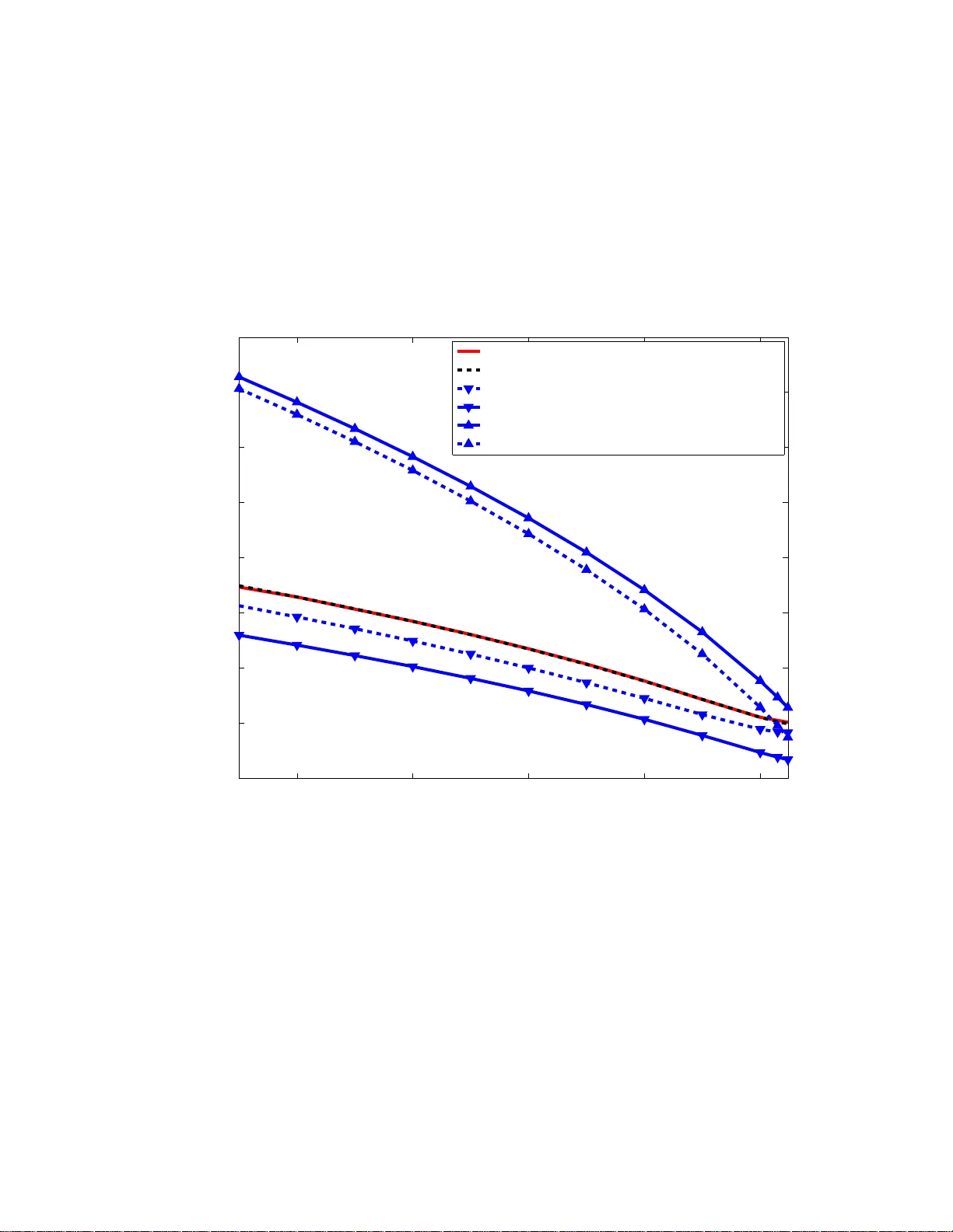
Capacity of The Discrete- T ime Non-Coherent Memoryless Rayleigh F ading Channels at Lo w SNR Z. Rezki and David Haccoun Departmen t of E lectrical En gineerin g, ´ Ecole Po lytechniq ue de Mo ntr ´ eal, Email: { zouh eir .rezki,david.hacc oun } @polymtl.ca, Franc ¸ ois Gagnon Departmen t of E lectrical En gineerin g, ´ Ecole d e tech nologie sup ´ erieure, Email: francois.g agnon @etsmtl.ca Abstract The capacity of a discrete-time memo ryless ch annel, in which successi ve symbols fade indepen- dently , and where the chann el state info rmation (CSI) is neither av ailab le at the transmitter nor at the receiver , is considered at lo w SNR. W e derive a closed form expression of the optimal capacity-ach ieving input distrib u tion at low signal-to-n oise ratio (SNR) and gi ve the exact capac ity of a non-coheren t channel at low SNR. Th e der iv ed relations allow to better u nderstan ding th e cap acity of n on-coh erent c hannels at low SNR an d bring an analytical answer to the peculiar behavior of the o ptimal input distribution observed in a previous work by Abo u Faycal, T rott and Shamai. Then , we comp ute the no n-coh erence penalty an d give a more precise ch aracterization of the sub-lin ear term in SNR. Finally , in or der to better understan d how the optimal input varies with SNR, upp er and lower bounds on the cap acity-achieving input are given. Index T erms Capacity , non -coher ent fading chann els, energy efficiency . I . I N T RO D U C T I O N In wireless communication , the channel esti mation at the re ceiv er is not often possible due, for instance, to the high m obility of the sender or the recei ver or both. Therefore, achieving reliable communication over fading channels where the channel state i nformation (CSI) is a vailable neither at the transm itter nor at th e receiver , is of a p articular interest. Es tablishing the performance limits, in terms of channel capacity , error probability , etc.., in such a non - coherent scenario has recently m otiv at ed e xtensive works (see for example [1], [2]). When CSI is a vailable at the recei ver , the channel capacity , commonly known as the coherent capacity has been studied by Ericson [3] for a Single Input Single Out put (SISO) channel and recently by many other authors for a Multipl e Input Multiple Output (MIMO) channel [4] [5]. Con versely , when CSI is not av ailabl e at bo th ends , computin g the channel capacity , kn own as the n on-coherent capacity , as well as com puting the optim al inp ut di stribution achieving this capacity , for both SISO and MIMO channels, i s a rather tedious task [6] [7]. The main difficulty in computi ng the non-coherent capacity relies on the fact that the capacity-achieving inp ut distribution is discrete with a finite numb er o f mass points , where one of them is located at the origin. The nu mber of these m ass points increases with the signal-to-noise ratio (SNR) . Since no bound on the number of mass poin ts with respect t o SNR is actually av ailable, it is very diffi cult t o find closed form expressions for both the achie vable ca pacity and the opti mal input distribution for all SNR values. Fortunately , numerical computat ion of the capacity and the optimal input di stribution has b een made possible using the Khun-T ucker condition which is a n ecessary and suffi cient conditio n for o ptimality , for of a SISO channel [6] and for a MIM O channel [7]. Earlier in 1999, using a block fading channel, Marzetta and Hochwald ha ve obtained the structure of the optim al input, with explicit calculations for the special case of a SISO channel at h igh SNR values or with a large coherence ti me [8]. The non-coherent capacity was also computed as a function of th e numb er of transmit and recei ve antennas as well as the coherence time at high SNR in [9]. At a low SNR regime, it was also shown i n [9] that to a first order of magnitude of the SNR, there is no capacity penalty for not knowing the channel at the recei ver which is not the case at the high SNR regime. It has been well establ ished previously that at low SNR, ju st like in an add itive white Gaussian noise (A WGN) channel, the capacity of a fading channel varies linearly with the SNR regardless of whether or not the CSI is av ailable at t he recei ver [10], [11]. Recently , this power effi ciency at a low SNR regime or equiv alently at a lar ge channel bandwidth has motiv ated work towards a bet ter understanding of th e non-coherent capacity at a low SNR regime [1], [13], [14] for both SISO and MIMO channels usin g severa l fading models. In this p aper , we analy ze the capacity of a di screte time non-coherent memoryless Rayleigh fading SISO channel at l ow SNR. The main contributions of this paper are: 1) Deriv ati on o f an analytical closed form of the channel mutu al inform ation at low SNR, which m ay also be consi dered as a lower bo und on the channel mutual informati on for an arbitrary SNR value. 2) Deriv ati on of a fundam ental relation between the capacity-achie ving input distribution and the SNR value, from which an exact capacity expression is deduced at low SNR. 3) Deriv ati on of novel upper and lower boun ds on the non -zero mass po int location of the optimal in put, which allow to deduce lower and u pper bounds respectively on th e non- coherent capacity at low SNR. The paper is organized as foll ows. Section II presents the system mo del. In section III, we deriv e a closed form expression of the channel mutual informati on at low SNR whi ch is also a lower bound on the chann el mutual information at all SNR values. The optimal input d istribution as well as the non-coherent capacity are presented in Section IV. Numerical resul ts are reported in Section V and Section VI concludes the paper . I I . C H A N N E L M O D E L W e consider a discrete-tim e memoryl ess Rayleigh-fading channel given by: r ( l ) = h ( l ) s ( l ) + w ( l ) , l = 1 , 2 , 3 , ... (1) where l is the discrete-time ind ex, s ( l ) is the channel in put, r ( l ) is the channel out put, h ( l ) is the fading coef ficient and w ( l ) is an additive noise. More s pecifically , h ( l ) and w ( l ) are independent complex circular Gaussian random variables with m ean zero and v ariances σ 2 h and σ 2 w , respectively . T he inpu t s ( l ) is subject to an a verage po wer constraint, that is E [ | s ( l ) | 2 ] ≤ P , where E [ . ] indicates the expected value. It is assumed that the channel state information is a vailable neither at the transmitter nor at t he recei ver . Ho wever , e ven thou gh t he exact values of h ( l ) and w ( l ) are n ot known, their statisti cs are, at both ends. Model (1) appears for example du ring the decomposition of a wideband channel into parallel noninteracting channels, or w hen a narrow-band s ignal i s hopped rapidly over a lar ge set of frequencies, o ne symbol per hop [1]. Since the channel defined in (1) is stationary and m emoryless, the capacity achie v ing statist ics of the input s ( l ) are also m emoryless, independ ent and id entically distri buted (i.i.d). Th erefore, for sim plicity we may drop t he time in dex l in (1). Consequently , the dist ribution of the channel output r conditio ned on the inp ut s can b e o btained after averaging out t he random fading coef ficient h , yield ing: f r | s ( r | s ) = 1 π ( σ 2 h | s | 2 + σ 2 w ) exp  −| r | 2 σ 2 h | s | 2 + σ 2 w  . (2) Noting th at in (2), the conditional out put distribution depends only on the squared magnitudes | s | 2 and | r | 2 , we will no longer be concerned wit h complex quanti ties but only wit h their squared magnitudes. Condition ed on the input, | r | 2 is chi-square distributed with two degrees of freedom: f | r | 2 | s ( t | s ) = 1 ( σ 2 h | s | 2 + σ 2 w ) exp  − t σ 2 h | s | 2 + σ 2 w  . (3) Normalizing to unit variance, let y = | r | 2 /σ 2 w and let x = | s | σ h σ w . Then (3) may be written more con veniently as: f y | x ( y | x ) = 1 (1 + x 2 exp  − y 1 + x 2  , (4) with t he ave rage p ower constraint E [ x 2 ] ≤ a , where a = P σ 2 h /σ 2 w is th e SNR per symbol ti me. I I I . T H E C H A N N E L M U T UA L I N F O R M A T I O N For the chann el (4), the mutual information is given by [12]: I ( x ; y ) = Z Z f y | x ( y | x ) f x ( x ) ln f y | x ( y | x ) f ( y ; x ) ( y ; x ) dxdy . (5) The capacity of channel (4) is th e supremum C = sup E [ x 2 ] ≤ a I ( x ; y ) (6) over al l input distributions t hat meet the constraint power . The existence and uniqueness of such an input dist ribution was established in [6]. More specifically , the optimal input distribution for channel (4) is d iscrete with a finite number o f mass p oints, where one of th em is necessarily null. That is, the capacity (6) is expressed by C = max E [ x 2 ] ≤ a N − 1 X i =0 p i Z ∞ 0 f y | x i ( y | x i ) ln " f y | x i ( y | x i ) P j p j f y | x j ( y | x j ) # dy , (7) where x 0 = 0 < x 1 < x 2 . . . < x N − 1 are th e m ass point locations and where p 0 , p 1 . . . , p N − 1 their probabilities respectiv ely . Th is optimization problem is very difficult sin ce th e number of discrete m ass poi nts, the optim um probabilities and their locations are unknown. In [6], numerical ev aluation of t he capacity and the optimu m in put distribution was given using the Khun-T ucker condition which is n ecessary and suf ficient for optimality . The authors have found empirically that two mass points are optimal for low SNR and that the number of mass points increases m onotonically with SNR. M any oth er papers hav e used these results in order to furth er understand t he non-coherent capacity and the optimal input dist ribution behavior as the SNR approaches zero [13], [14]. Since we focus on the low SNR regime, we may use in (7) a discrete i nput distribution with two m ass p oints, where one of t hem is null, to obtain the optimal capacity at low SNR. Furthermore, thi s on-off signaling also provides a lo wer bound on the non-coherent capacity for all SNR values. Clearly , using com puter simulati on, i t was shown in [6] that on-off signaling provides a tigh t l ower bound on the capacity for th e SNR values considered. That is, a lower bound o n the capacity may be expressed by : C LB = max E [ x 2 ] ≤ a I LB ( x ; y ) , (8) where I LB ( x ; y ) is a lower bound on the channel mutual information I ( x ; y ) given b y: I LB ( x ; y ) = I LB ( x 1 , p 1 ) = 1 X i =0 p i Z ∞ 0 f y | x i ( y | x i ) ln " f y | x i ( y | x i ) P j p j f y | x j ( y | x j ) # dy , (9) and the aver age constraint power b ecomes: p 1 x 2 1 ≤ a . Note that the opt imization problem in (8) i s less complex than in (7) since we deal with only two unknowns p 1 ND x 1 . Furthermore, it is proven below that further simplification s can be obt ained, usi ng the fact that I LB ( x 1 , p 1 ) is monoto nically increasing in x 1 and thus the problem at hand may be reduced to a si mpler maximization problem wit hout constraint . W e su mmarize thi s result in lemma 1. Lemma 1: The opt imal capacity at low SNR and a lower bound on it for all SNR values is giv en by: C LB = max x 1 ≥ √ a I LB ( x 1 , a ) , (10) where I LB ( x 1 , a ) is the channel m utual informatio n for a giv en mass point location x 1 and a giv en SNR va lue a . Furthermore, I LB ( x 1 , a ) may be written as: I LB ( x 1 , a ) =            a − a h ln (1+ x 2 1 ) x 2 1 + 1 1+ x 2 1 + x 2 1 1+ x 2 1 · 1 F 2  1 , 1 x 2 1 , 1 + 1 x 2 1 , − (1+ x 2 1 )( x 2 1 − a ) a i − ln  1 − a x 2 1  − ln  1 + a (1+ x 2 1 )( x 2 1 − a )  if x 1 > √ a, 0 if x 1 = √ a (11) where 2 F 1 ( · , · , · , · ) is t he Gauss hypergeometric function. Pr oof: For con venience, the proof is presented in Appendix I. In Lem ma 1, t he existence of a maximum for a given SNR value a is guaranteed by t he continuity of I LB ( x 1 , a ) and t he fact that it is bounded with respect to x 1 over the interva l [ √ a, ∞ [ . This can be readily s een in Fig. 1 where we have plotted the lower bound I LB ( x 1 , a ) for diffe rent values of a . As can be seen in Fig. 1, I LB ( x 1 , a ) has a m aximum for the 3 SNR regimes. The existence of such a maximum is also rigorously established in Appendix I. Clearly , as was discussed in Appendix I, t he maximizati on (10) is reduced to solvi ng the equation ∂ ∂ x 1 I LB ( x 1 , a ) for a given SNR value a . Ideally , an analytical s olution would provide an insight as to how the non-coherent capacity and the optimal input distribution vary wit h the SNR. Howe ver , solving such an equation for arbitrary SNR values is ve ry ambit ious since it inv olves an analytical solut ion to a transcendental equations. Nevertheless, it is of interest to focus on the low SNR regime to get the benefit of som e advantageous simpli fications i n order to elu cidate the non-coherent capacity beha v ior at low SNR. I V . N O N - C O H E R E N T C A P AC I T Y A T L OW S N R In this section, we will use Lemm a 1 to deriv e a fundam ental analytical relation between the optimal input di stribution at a low SNR regime and the particular SNR value a . W e show in Theorem 1 t hat th is fundamental relation holds up to an o rder o f a strictly less than 2. A s is shown below , the deri ved relation is very us eful since it all ows computi ng the optimal input distribution for a given SNR v alue a while providing a rigo rous characterization as to how the non zero mass point locatio ns and their probabilities vary with a . Moreov er , the derived relation may be used to compute th e exact no n-coherent capacity at low SNR v alues. A. A fundamenta l r elati on between the optimal i nput d istribution and the SNR W e p resent the fundamental relation between the opt imal input distribution and the SNR value in the following Theorem: Theor em 1: At a low SNR value a , th e optim al input probabi lity distribution for an order of magnitude of a strictly less than 2, is giv en by: f x ( x ) =      x 1 with p robability p 1 = a x 2 1 , 0 with p robability p 0 = 1 − p 1 , (12) where x 1 is th e s olution of the equation: x 2 1 − (1+ x 2 1 ) ln(1+ x 2 1 ) − π  a x 2 1 + x 4 1  1 x 2 1 csc  π x 2 1   1 + x 2 1 − π cot  π x 2 1  + ln  a x 2 1 + x 4 1  = 0 . (13) Furthermore, the non-coherent channel capacity is given by: C ( a, x 1 ) = a − a · ln (1 + x 2 1 ) x 2 1 − a 1+ 1 x 2 1 · π csc  π x 2 1   1 x 2 1 + x 4 1  1 x 2 1 1 + x 2 1 (14) Pr oof: For con venience, the proof is presented in Appendix II. Clearly , (13) is also a transcendental equation , for whi ch determining an analytical solut ion is a very t edious task. Al though it is very in volve d to deriv e an analytical s olution o f (13) in the form of x 1 = f ( a ) , it is of interest from an engineering point of view , to resolve (13) numerically and obtain the op timal x 1 for a given SNR value a . One may then get the value of the non-coherent capacity by replacing in (14) the ob tained value of x 1 . Moreove r , (13) provides some insight on t he behavior of x 1 as a tends towa rd zero. For example, usi ng (13), one may determine th e l imit of x 1 as a t ends toward zero. T o see this, let M be this lim it and let us assume that M is finite. From Appendix II , we know that for the op timal input di stribution, the non-zero mass p oint location x 1 is greater than one. Thus, its limi t as a tends toward zero is greater or equal than one M ≥ 1 . Then, taki ng the lim its on bot h sides of (13) as a goes to zero yields: M 2 − (1 + M 2 ) ln (1 + M 2 ) = 0 . (15) That is, if M is finite, it would be equal to zero, t he uniqu e soluti on to (15), but this is impo ssible since M ≥ 1 . Hence, con sistently with [6], [13], lim a → 0 x 1 = ∞ . Furthermore, we have found that (13) may be written in a mo re con venient way as: a = exp  x 2 1 W  k , ϕ ( x 1 )  − x 2 1 + π cot  π x 2 1  + ln ( x 2 1 ) + ln (1 + x 2 1 ) − 1  , (16) with k = − 1 if a ≤ a 0 and k = 0 elsewhere , and where W ( · , · ) is the Lam bert functi on, with ϕ ( x ) giv en by : ϕ ( x ) = − sin ( π x 2 )( − x 2 + ln (1 + x 2 ) + x 2 ln (1 + x 2 )) π x 2 · exp − π cot  π x 2  x 2 + 1 + 1 x 2 ! . (17) Also, a 0 is t he sol ution of (13) for x 1 = x 0 , where x 0 is t he root of the equation ϕ ( x ) = − 1 e . The num ber − 1 e comes ou t in our analysis from the fact that it is the uniq ue point sh ared by the principal branch of the Lambert function W (0 , x ) and the branch with k = − 1 , W ( − 1 , x ) . That is W (0 , − 1 e ) = W ( − 1 , − 1 e ) . This guarantees the continuity of a in (16 ) for all x 1 values. Numerically , we hav e found th at a 0 = 0 . 05 82 and x 0 = √ 3 . 93388 . Hence, (16) may al so be viewed as a fundam ental relation between the op timal input distribution and a for discrete-time non-coherent memoryless Rayleigh f adi ng channels at lo w SNR. On th e other hand, (16) provides the glo bal answer as to how the non-zero mass point locati on of t he opti mal on-off sign aling and the SNR are lin ked to gether . For this purpose, a sim ple analysis of (16) has been done and some i mportant results are recapitulated i n the following corollary . Cor ollary 1: At low SNR, we have: 1) For all a ≤ a 0 , a 0 = 0 . 0582 , a is an decreasing functi on wi th respect to x 1 and for all a > a 0 , a is an increasing function of x 1 . 2) For all a , x 1 ≥ x 0 , where x 0 = √ 3 . 93388 . 3) lim x 1 →∞ a = 0 . Corollary 1 agrees with [6] where it was shown us ing computer si mulation that the no n-zero mass point location passes through a minimum before moving upward. Howe ver , by specifying the edge poin t ( x 0 , a 0 ) , Corollary 1 gives a mo re precise characterization concerning this p eculiar beha vior of the non-zero mass point locations. Furthermore, Corollary 1 also refines the lower bound on x 1 , x 1 > 1 and deriv es x 0 as an improved lower bound on th e non-zero mass poin t location at low SNR. Moreover , from (16), we may write: ln ( a ) + x 2 1 = x 2 1 W  k , ϕ ( x 1 )  + π cot  π x 2 1  + ln ( x 2 1 ) + ln (1 + x 2 1 ) − 1 . (18) It is then easy to check that the right hand si de (RHS) of (18 ) is a decrea sing function of x 1 for x 1 < x 0 , which yields an upper bound on x 1 : x 2 1 ≤ − ln ( a ) + ξ 0 , (19) where ξ 0 = ln ( a 0 ) + x 2 0 , whi ch is again con sistent with the upper bound deriv ed in [13]. Note that the upper bo und (19) is valid for all a ≤ a 0 whereas the upper b ound provided in [13] holds for a ≪ a 0 for wh ich ξ 0 is negligible. On t he other h and, combi ning (19) and the lower bound on x 1 provided in Corollary 1 on e may obtain: a α x 2 0 ≤ a α x 2 1 ≤ a α ( ξ 0 − ln ( a )) . (20) for all α > 0 . That i s: lim a → 0  a α x 2 1  = 0 , (21) which means that a α tends to ward zero faster than x 2 1 does tow ard infinity . This result may also be used t o gain further insi ght on the capacity behavior at low SNR. For instance, from (14), we m ay write the non-coherent capacity as: C ( a ) = a + o ( a ) , (22) where o ( a ) = − a · ln (1+ x 2 1 ) x 2 1 − a 1+ 1 x 2 1 · π csc „ π x 2 1 «„ 1 x 2 1 + x 4 1 « 1 x 2 1 1+ x 2 1 , meanin g that th e non-coherent capacity var ies li nearly with a at low SNR and hence non-coherent communication at low SNR may be qualified as energy efficient communi cation. B. Ener gy efficiency and non-coher ence pena lty In general, the capacity of a channel including a Gauss ian channel and a Rayleigh channel var ies linearly at low SNR [13]. The dif ference between these channels in terms of capacity can only be explained by the sub-lin ear term o ( a ) in (22). The sub-li near term has been defined in [13] as: ∆( a ) := a − C ( a ) . (23) At low SNR, the sub-l inear term ∆( a ) i s also related to t he ener gy-ef ficiency . let E n be t he transmitted energy i n Joules per informatio n nat, then we have: E n σ 2 w · C ( a ) = a. (24) Using (23), we can write: E n σ 2 w = 1 1 − ∆( a ) a ≈ 1 + ∆( a ) a , (25) where th e appro ximation ho lds i f ∆( a ) a is suffi ciently small . Note that if ∆( a ) a → 0 , (26) then from (23) and (25), we have respectiv ely : C ( a ) ≈ a (27) E n σ 2 w ≈ 1 , (28) which implies that the hi ghest ener gy effic iency of -1.59 (dB) per informati on bit could be theo- retically achie ved. For a Gaussian channel and a fading channel under the coherent assumpt ion, the sub-linear terms are respectiv ely give n by [13]: ∆ AW GN ( a ) = 1 2 a 2 + o ( a 2 ) (29) ∆ coher ent ( a ) = 1 2 E [ k h k 4 ] a 2 + o ( a 2 ) (30) For a non-coherent Rayleigh fading channel, the sub-li near term can be computed using (14): ∆( a ) = a · ln (1 + x 2 1 ) x 2 1 + a 1+ 1 x 2 1 · π cs c  π x 2 1   1 x 2 1 + x 4 1  1 x 2 1 1 + x 2 1 . (31) Note that at very low SNR and following (31), ∆( a ) a con ver ges to zero m aking the non -coherent Rayleigh channel als o energy ef ficient. Howe ver , as SNR increases, the con ver gence of ∆( a ) a to zero is sl ower than ∆ AW GN ( a ) a and ∆ coher ent ( a ) a . This could be seen from (21) ind icating that x 1 con ver ges slower to infinity than a does to zero. T o illustrate this, as an example, let us calculate the v alue of ∆( a ) a for an SNR value a = − 30 dB . Follo wi ng (31), we can write: ∆( a ) a = ln (1 + x 2 1 ) x 2 1 + a 1 x 2 1 · π cs c  π x 2 1   1 x 2 1 + x 4 1  1 x 2 1 1 + x 2 1 . (32) Solving (16) for a = − 30 d B with respect to x 2 1 yields: x 2 1 ≈ 4 . 96815 . T hen, sub stitutin g th is value in (32), we obt ain ∆( a ) a ≈ 49% . Note that for A WGN and coherent Rayleigh fa ding channels, ∆ AW GN ( a ) a and ∆ coher ent ( a ) a are at the sam e order of magnitud e than the SNR value in this case. It takes a lower SNR for non-coherent comm unication to achiev e th e s ame energy ef ficient as A WGN and coherent Rayleig h fading channels. In the range of SNR values of interest, we may define the non -coherence penalty per SNR as: C coher ent ( a ) − C ( a ) a . (33) where C coher ent is the channel capacity und er coherent ass umption. N ow , from [1 3], we can writ e C coher ent as: C coher ent ( a ) = a + O ( a ) = a + o ( a 2 − α ) , (34) for any 1 > α > 0 . Recalling that the non-coherent capacity i n (14) was obt ained using series decompositio n to an order strictly smaller than 2, then combi ning (14) and (34), we derive the exact non-coherence penalty per SNR up to t his order: C coher ent ( a ) − C ( a ) a = C coher ent − C C coher ent = ln (1 + x 2 1 ) x 2 1 + a 1 x 2 1 · π csc  π x 2 1   1 x 2 1 + x 4 1  1 x 2 1 1 + x 2 1 (35) Now using (21), dividing both sides of (35) by a α , ( α > 0 ) and taking the limit as a tends t o zero yi elds: C coher ent ( a ) − C ( a ) ≫ a 1+ α , (36) where ≫ means: lim a → 0 C coher ent ( a ) − C ( a ) a 1+ α = ∞ . (37) Inequality (36) ind icates th at not only the n on-coherent capacity is much greater t han a 2 as was established in [1], but more precisely , it is much greater than a 1+ α since a 1+ α ≫ a 2 , 1 > α > 0 . Again, th is result is in full agreement with [13]. In thi s subsection , we hav e dis cussed exact closed form s of the optim al input d istribution and the non-coherent capacity b ased on the fund amental relation (13) or equ iv alently (16). Howe ver , one may be interested in deriving simp ler lower and u pper b ounds on these quantit ies in order to bett er und erstand how they vary with the SNR value a . This is di scussed next. C. Up per and lower bounds on t he non-coher ent cap acity Considering (16), si nce we are interested i n t he low SNR regime, we assume for simpli city that a ≤ a 0 . Thus the L ambert functi on in (16) is t he branch with k = − 1 , th at is W ( − 1 , x ) . A lo wer bound on th e non-coherent capacity i s easily obtained by com bining (19) and (14) and will be referred to as C LB ( a ) . W e now derive the l ower bound on the optimal non-zero mass point location and the upper bound on the non-coherent capacity in Theorem 2. Theor em 2: At low SNR values a , a lower boun d on th e optim al non-zero mass point l ocation is given by: x 1 ,LB = y v u u t − W − 1 , ϕ  y − ln  − ϕ ( y )   ! , (38) where y = q 1 + ln 1 a . F urthermore, an upper bound on the non-coherent capacity can be obtained from (14) as: C U B ( a ) = C ( a, x 1 ,LB ) (39) Pr oof: For con venience, the proof is presented in Appendix III. V . N U M E R I C A L R E S U LT S A N D D I S C U S S I O N The curves in Fig. 2 show respectively , the non-zero mass point location of the capacity- achie ving input distribution x 1 obtained using maximization (10), and the on e obtained us ing relation (13) or equiva lently (16). As can be seen from Fig. 2, th e two curv es are undis tinguishabl e at low SNR, confirming that (17) i s exact at low SNR. As t he SNR increases, a small discrepancy between the two curves starts to appear . This i s expected since (16) holds for u p to an order o f magnitude strictly smaller than 2 and thu s for small SNR values, (but not small er than about 2 . 10 − 2 ), a di screpancy m ay appear . Nev ertheless , ev en for an SNR greater than 2 . 10 − 2 , the curve obtained u sing (16) is very instructive especially as i t follows the same shape as the one obtained by si mulation results. An in teresting future work would be to use (17) in order to understand why a new mass po int should appear as the SNR i ncreases. It should b e mention ed that th e discrepancy observed in Fig . 2 may be rendered as small as desired using high o rder series expansion. Howe ver , the analysis would be unrew arding ly too complex. Figure 3 depicts the non-coherent capacity curves. Again, t he curve obtained by computer sim- ulation and the one obtained using (14) are un distingui shable. More interestingly , the discrepancy observed at not v ery lo w SNR values in Fig. 2 has v anished, impl ying that the ca pacity is not very sensitive to the non-zero mass poi nt lo cation. Al so shown in Fig. 3 is the linear approximati on C ( a ) = a , which i s an upper boun d on the capacity . As can be no ticed in Fig. 3, the lin ear approximation follows the sam e shape as the exact non-coherent capacity curves at low SNR and becomes quite loose for SNR values greater than 10 − 2 . This impli es that the s ub-linear term defined i n (23) is much more i mportant at these SNR values. This can be seen in Fig. 4 where we have plotted the non-coherence penalty percentage giv en by (35). Figure 4 confirms that there is n o sub stantial gain in the channel kn owledge in a capacity sense at very low SNR, thus indicating that non -coherent com munication is almost as power -effi cient as A WGN and coherent communication s. As the SNR increases, a non-coherence penalty begins to app ear reaching up to 70 % . The deriv ed upper and lower bounds on the non zero mass point locations given respectively by (19) and (38) as well as well as t he b ounds deri ved in [13] are plot ted in Fig. 5 along with the exact curves at low SNR. As can be s een in Fig . 5, the upper bound in [13], albeit tighter than (19), crosses the exact curves at about 2 . 1 0 − 2 . At these not so low SNR values, the derived bound in [13] is no longer an upper bound, consi stently with our discussio n in Subsection IV -A. On the other hand, the lower bound (38) is ti ghter than t he o ne deriv ed in [13] for all SNR values. V I . C O N C L U S I O N In this paper , we have addressed t he analysis of the capacity of discrete-time non-coherent memoryless Rayleigh fading channels at low SNR. W e ha ve computed explicit ly the channel mutual information at low SNR which is also a lowe r b ound on the channel mut ual information, albeit no t necessarily at low SNR values. Using the deri ved expression of the channel mutual informati on, we ha ve been able to provide a fundamental relation between the non-zero mass point location of the capacity-achie ving inpu t distribution and the SNR. This fundamental relation brings th e complete ans wer about how the optimal input distribution varies with the power constraint at low SNR. It als o provides an analytical explanation on what was previously observed through computer simulatio n in [6] about the peculiar behavior of the non-zero mass poi nt location at low SNR values. The exact non-coherent capacity has been derived and insights on th e capacity beha vi or which can be gained throu gh functi onal analysi s has been shown. In order to better understand how the n on-zero m ass poi nt l ocation varies wi th t he SNR, we hav e also derived lo wer and upper bounds which hav e been compared to recently derived bound s. The ne wl y derived lower bound is tighter for all SNR v alues of interest, whereas somewhat looser , the upper bound was shown to hold for larger SNR values. A P P E N D I X I P R O O F O F L E M M A 1 For con venience, we will use f ( x ) i nstead o f f x ( x ) to denote the p robability density function of the random variable x at the v alue x . W e first prove that I LB ( x ; y ) is a s trictly mo notonically increasing functi on wit h respect to x 1 . 1 Diffe rentiating (9) with respect t o x 1 yields ∂ ∂ x 1 I LB ( x 1 , p 1 ) = p 1 Z ∞ 0 ∂ ∂ x 1 f ( y | x 1 ) ln  f ( y | x 1 ) f ( y )  dy (I.40) Diffe rentiating (4), we obtain: ∂ ∂ x 1 f ( y | x 1 ) = 2 x 1 (1 + x 2 1 ) 2  y − (1 + x 2 1 )  f ( y | x ) (I.41) Substitutin g (I.41) in (I.40) yields: ∂ ∂ x 1 I LB ( x 1 , p 1 ) = 2 p 1 x 1 (1 + x 2 1 ) 2 Z ∞ 0  y − (1 + x 2 1 )  f ( y | x 1 ) ln  f ( y | x 1 ) f ( y )  dy (I.42) Let g ( y ) be defined as g ( y ) = ln  f ( y | x 1 ) f ( y )  . No w , we need the following lemma. Lemma 2: Let f ( y ) b e a probability d ensity function with mean m . If g ( y ) is a strictly monotonicall y increasing fun ction t hen Z ( y − m ) f ( y ) g ( y ) > 0 (I.43) Pr oof: The p roof follows along sim ilar lines as L emma 1 in [6]. T o apply Lemma 2, it is suf ficient to note that f ( y ) f ( y | x 1 ) = p 1 + p 0 (1 + x 2 1 ) exp  y  1 1 + x 2 1 − 1)  (I.44) 1 Note that the technic used here to prove that I LB ( x ; y ) is strictly monotonically increasing function with respect t o x 1 follo ws along the same lines as the techn ic used to establish that the optimal input distr ibution has necessarily a mass point at zero in [6], albeit the two technics hav e strictly dif ferent objectiv es is strictly decreasing wit h respect to y because the exponent of the exponential function is negati ve, therefore f ( y | x 1 ) f ( y ) is st rictly i ncreasing and so is g ( y ) . Finally , using the fact t hat (1 + x 2 1 ) is th e m ean o f f ( y | x 1 ) and applying Lemma 2 t o (I.42), we obtain: ∂ ∂ x 1 I LB ( x 1 , p 1 ) > 0 , (I.45) which means t hat I LB ( x 1 , p 1 ) is stri ctly increasing with respect t o x 1 . Consequently , the av erage power constraint hold s with equality . That is E [ x 2 ] = p 1 x 2 1 = a . Hence (8) is equiv alent to:      C LB = max x 1 ≥ √ a I LB ( x 1 , p 1 ) p 1 x 2 1 = a. (I.46) Next, we prove t he existence o f t he maximum in (I.46). Clearly , I LB ( x 1 , p 1 ) is now a functio n of x 1 and a since p 1 x 2 1 = a . That x 1 ≥ √ a follows automatically from th e fact th at p 1 ≤ 1 . On the ot her hand, I LB ( x 1 , p 1 ) in (9) is positive-definite and continue with respect to x 1 and p 1 and thus s o is I LB ( x 1 , a ) for a given SNR value a . M oreover I LB ( x 1 , a ) is upper-bounded over the interval [ √ a, ∞ [ otherwise, one would hav e, for som e SNR v alue, say a 0 : ∀ ǫ > 0 , ∃ x 0 1 > √ a 0 | I LB ( x 0 1 , a 0 ) > ǫ. (I.47) But this statement also means that the channel mutual informatio n-an upper bound on I LB ( x 1 , a 0 ) - is unb ounded for a 0 which contradi cts the fact that the capacity exists for all SNR values as proven i n [6]. Hence, I LB ( x 1 , a ) is necessarily upper-bounded. Furthermore, the continuity of I LB ( x 1 , a ) over [ √ a, ∞ [ implies that the upper-bound is eith er achiev ed at a finit e value x 1 or at ∞ . The last case is howe ver imposs ible. T o see this, it is suf ficient to observe that for a giv en a , as x 1 goes to infinity , p 1 tends tow ard zero. Thus following (9 ), lim x 1 →∞ I LB ( x 1 , a ) = I LB ( ∞ , 0) = 0 , and consequentl y I LB ( x 1 , a ) = 0 for all x 1 ∈ [ √ a, ∞ [ wh ich is i mpossibl e since th e d iscrete input distribution x and the output y are dependent. That is, the upper bound is achie ved at a finite value x 1 and this proves the e xistence o f the maximum i n (I.46). Moreover , since th e maxim um is not at the borders of [ √ a, ∞ [ , we necessarily have at the maxi mum ∂ ∂ x 1 I LB ( x 1 , a ) = 0 . Finally , in order to prove (11), we directly compute the lower bound I LB ( x 1 , p 1 ) from (9): I LB ( x 1 , p 1 ) = p 0 Z ∞ 0 f ( y | 0) ln ( f ( y | 0)) dy | {z } I 1 − p 0 Z ∞ 0 f ( y | 0) ln ( f ( y )) | {z } I 2 + p 1 Z ∞ 0 f ( y | x 1 ) ln ( f ( y | x 1 )) | {z } I 3 − p 1 Z ∞ 0 f ( y | x 1 ) ln ( f ( y )) | {z } I 4 (I.48) I 1 and I 3 may be easil y comp uted: I 1 = p 0 Z ∞ 0 e − y ln ( e − y ) dy = − p 0 = 1 − p 1 (I.49) I 3 = p 1 Z ∞ 0 1 1 + x 2 1 e − y 1+ x 2 1 ln  1 1 + x 2 1 e − y 1+ x 2 1  dy = − p 1  1 + ln ( 1 + x 2 1 )  (I.50) I 2 = p 0 Z ∞ 0 e − y ln  p 0 e − y + p 1 1 + x 2 1 e − y 1+ x 2 1  dy = Z ∞ 0 p 0 e − y ln  p 0 e − y  dy | {z } I 21 + Z ∞ 0 p 0 e − y ln 1 + p 1 p 0 (1 + x 2 1 ) e „ 1 − 1 1+ x 2 1 « y ! dy | {z } I 22 (I.51) I 21 can be easily computed: I 21 = p 0 [ln ( p 0 ) − 1] (I.52) In order to compute I 22 , let α = 1 + x 2 1 and β = p 1 p 0 α = p 1 (1 − p 1 ) α . Thus, I 22 may be written: I 22 = p 0 α α − 1 Z ∞ 1 t 1 − 2 α α − 1 ln (1+ β t ) dt = p 0 α α − 1 (  1 − α α t − α α − 1 ln (1 + β t )  ∞ 1 − 1 − α α β Z ∞ 1 t − α α − 1 1 + β t dt ) (I.53) The integral on th e RHS of (I.53) may be computed as [15]: Z ∞ 1 t − α α − 1 1 + β t dt = α − 1 αβ · 2 F 1  1 , 1 + 1 α − 1 , 2 + 1 α − 1 , − 1 β  (I.54) Substitutin g (I.54) in (I.53), we obtain: I 22 = p 0  ln (1 + β ) + α − 1 α 2 F 1  1 , 1 + 1 α − 1 , 2 + 1 α − 1 , − 1 β  , (I.55) and thus comb ining (I.51), (I.52) and (I.55), yields: I 2 = p 0 [ln ( p 0 ) − 1] + p 0  ln (1 + β ) + α − 1 α · 2 F 1  1 , 1 + 1 α − 1 , 2 + 1 α − 1 , − 1 β  . (I.56) The integral I 4 may be computed similarly . W e sk ip the d etails and give below the final result: I 4 = p 1 ln ( p 0 ) − p 1 α + p 1  ln (1 + β ) + ( α − 1) · 2 F 1  1 , 1 α − 1 , 1 + 1 α − 1 , − 1 β  . (I.57) Follo wing (I.48), (I.49), (I.50), (I.56), (I.57) and u sing the fact that : 2 F 1  1 , 1 α − 1 , 1 + 1 α − 1 , − 1 β  + 1 − p 1 p 1 · 2 F 1  1 , 1 + 1 α − 1 , 2 + 1 α − 1 , − 1 β  = 1 , (I.58) we o btain: I LB ( x 1 , p 1 ) = − ln (1 − p 1 ) + p 1  x 2 1 − ln (1 + x 2 1 )  − ln (1 + β ) − p 1 ( α − 1) α  ( α − 1) · 2 F 1  1 , 1 α − 1 , 1 + 1 α − 1 , − 1 β  + 1  . (I.59) Combining (I.59) and (I.46) yields (11) whi ch complet es the proof of Lemm a 1. A P P E N D I X I I P R O O F O F T H E O R E M 1 At low SNR, a dis crete input di stribution wit h two mass p oints, one of them located at zero, achie ves the non-coherent capacity [6]. That p 1 = a/x 2 1 was proven in Appendix I. Therefore, (12) is true. T o derive (13), it is a matter of series expansion calculus. Before proceeding, it should be reminded that for the optimal input distribution given in Theorem 1, the non-zero m ass poi nt locati on x 1 is greater than 1 ( x 1 > 1) [6], [13]. Then, series expansion of (11) to the second order , around the point ( x 1 , a ) = ( x 1 , 0) , where x 1 is an arbitrary real greater than one, can be obtained using Math ematica: I LB ( x 1 , a ) =  (1 − log(1 + x 2 1 ) x 2 1 ) a + 1 2( x 2 1 − 1) a 2 + o ( a 2 )  − a 1 x 2 1  π x 2 1  x 2 1 (1 + x 2 1 )  − 1+ x 2 1 x 2 1 csc  π x 2 1  a + π  x 2 1 (1 + x 2 1 )  − 1+ x 2 1 x 2 1 csc  π x 2 1  x 2 1 a 2 + o ( a 2 )  , (II.60) where the symbol ◦ ( a n ) represents a function say g ( x 1 , a ) , such that lim a → 0 g ( x 1 ,a ) a n = 0 . Since x 1 > 1 , then there exists ǫ > 0 such that 1 + 1 x 2 1 < 2 − ǫ . Thus, (I.40) may be w ritten as: I LB ( x 1 , a ) =  1 − log(1 + x 2 1 ) x 2 1  a − π x 2 1  x 2 1 (1 + x 2 1 )  − 1+ x 2 1 x 2 1 csc  π x 2 1  a 1+ 1 x 2 1 + o ( a 2 − ǫ ) , (II.61) which represents series expansion t o an order strictly less than 2. Up t o this order , we may make some abuse o f n otation, drop the term o ( a 2 − ǫ ) and writ e (II.61) as: I LB ( x 1 , a ) =  1 − log(1 + x 2 1 ) x 2 1  a − π x 2 1  x 2 1 (1 + x 2 1 )  − 1+ x 2 1 x 2 1 csc  π x 2 1  a 1+ 1 x 2 1 . (II.62) Maximizing (I.42 ) wi th respect to x 1 > 1 is equivalent t o: min x 1 > 1 " log(1 + x 2 1 ) x 2 1 + π x 2 1  x 2 1 (1 + x 2 1 )  − 1+ x 2 1 x 2 1 csc  π x 2 1  a 1+ 1 x 2 1 # . (II.63) As was proven in Appendix I, at the maximum, we hav e necessarily ∂ ∂ x 1 I LB ( x 1 , a ) = 0 . Diffe rentiating (II.63) with respect to x 1 yields (13 ). Finall y , (14) follows from (II.62). This completes the proof of Theorem 1. A P P E N D I X I I I P R O O F O F T H E O R E M 2 For a < a 0 and x 1 > x 0 , (16) m ay be written as: a ( x 1 ) = exp  x 2 1 W  − 1 , ϕ ( x 1 )  − x 2 1 + π cot  π x 2 1  + ln ( x 2 1 ) + ln (1 + x 2 1 ) − 1  . (III.64) Moreover , it is easy to check that a in (III.64) is a decreasing function wi th respect to x 1 and that: − x 2 1 + π cot  π x 2 1  + ln ( x 2 1 ) + ln (1 + x 2 1 ) − 1 > 1 , (III.65) for x 1 > x 0 . Thus, usi ng (III.64) and (III.65), we have: a ( x 1 ) > a lb ( x 1 ) = exp  x 2 1 W  − 1 , ϕ ( x 1 )  + 1  , (III.66) where a lb ( x 1 ) is a lower bou nd on a ( x 1 ) . Since a lb ( x 1 ) is also a d ecreasing fun ction wi th respect to x 1 , then for a low SNR value a , (III.66) may be seen as a lower bound on the o ptimal non -zero mass po int l ocation x 1 and we equivalently ha ve: x 1 > x 1 ,lb , (III.67) where x 1 ,lb is th e s olution of a lb ( x 1 ) = a . Next, we deriv e a lower bound on x 1 ,lb . Let us fix e a l ow SNR value a < a 0 and consider the function on t he RHS of (III.66) writ ten for s implicity as: a = exp  x 2 1 ,lb W  − 1 , ϕ ( x 1 ,lb )  + 1  , (III.68) or equi valently by lett ing y = q 1 + ln  1 a  : x 2 1 ,lb = y 2 − W  − 1 , ϕ ( x 1 ,lb )  . (III.69) Since − W  − 1 , ϕ ( x 1 ,lb )  > 1 for x 1 ,lb > x 0 , it is easy to see that y 2 > x 2 1 ,lb . Hence, using the fact that ϕ ( · ) and − W  − 1 , ·  are stri ctly in creasing function s, we hav e: x (1) 1 ,LB = y q − W  − 1 , ϕ ( y )  < x 1 ,lb = y q − W  − 1 , ϕ ( x 1 ,lb )  , (III.70) where t he sup erscript ( 1 ) on the left hand s ide of (III.70) m eans a first lower bound. Next we improve the lower bo und x (1) 1 ,LB to obt ain a tighter one. But before going on , we remind this result from [16] which aims at resol ving transcendental equati ons in volving Lambert functio n iterativ ely using self-mapping techniq ues: Lemma 3: For the region specified by x < 1 and − 1 e < y < 0 , an infinite-ladder solu tion t o the equation: y ( x ) = xe x (III.71) is easily id entified as x ( y ) = L < ( y ) , (III.72) with t he ladder L < ( y ) defined as L < ( y ) = − ln ln ln ( ... ) − y − y ! . ( III.73) Pr oof: T he proof and m ore details concerning the Lambert function can be found in [16]. Clearly , using (III.73) and t he fact that the solu tion of (III.71) is als o x ( y ) = W ( − 1 , y ) , one can obtain a sim ple upper bound on t he Lambert function in the i nterval of interest: W ( − 1 , y ) ≤ ln ( − y ) − ln  − ln ( − y )  . (III.74) Since for x 1 ,lb > x 0 , ϕ ( x 1 ,lb ) ∈ ] − 1 e , 0[ and W ( − 1 , ϕ ( x 1 ,lb )) < 0 , then applyi ng (III.74) to ϕ ( x 1 ,lb ) yields: W ( − 1 , ϕ ( x 1 ,lb )) ≤ ln  − ϕ ( x 1 ,lb ) − ln  − ϕ ( x 1 ,lb )   (III.75) ≤ ln  − ϕ ( y ) − ln  − ϕ ( x 1 ,lb )   (III.76) ≤ ln  − ϕ ( y )  . (III.77) Inequality (III.76) holds because y > x 1 ,lb and ϕ ( · ) is an in creasing function, likewise (III.77) follows from the fact t hat for x > x 0 , ϕ ( x ) > − 1 e and thu s 1 − ln  − ϕ ( x )  < 1 . Moreover , (III.77) implies y − ln  − ϕ ( y )  ≥ y − W ( − 1 , ϕ ( x 1 ,lb )) = x 1 ,lb (III.78) Applying again respectiv ely ϕ ( · ) and − W ( − 1 , · ) to both sides of (III.78) gives: x (2) 1 ,LB = y s − W  − 1 , ϕ  y − ln  − ϕ ( y )    ≤ y p − W ( − 1 , ϕ ( x 1 ,lb )) = x 1 ,lb . (III.79) Finally , to pro ve that x (2) 1 ,LB is tighter than x (1) 1 ,LB , it is sufficient to note that since ϕ ( x 1 ,lb ) ∈ ] − 1 e , 0[ , y > x 1 ,lb and ϕ ( · ) is an increasing function, then ϕ ( y ) ∈ ] − 1 e , 0[ and w e have consequentl y: y > y − ln  − ϕ ( y )  . Applying again respectiv ely ϕ ( · ) and − W ( − 1 , · ) to t his i nequality yield s: x (1) 1 ,LB = y q − W  − 1 , ϕ ( y )  ≤ y s − W  − 1 , ϕ  y − ln  − ϕ ( y )    = x (2) 1 ,LB . (III.80) Combining (III.79 ) and (III.80), we hav e: x (1) 1 ,LB ≤ x (2) 1 ,LB ≤ x 1 ,lb , (III.81) from whi ch (38) follows b y lett ing x (2) 1 ,LB = x 1 ,LB . Finally , (39) may b e o btained by applying (14) to x 1 ,LB . This comp letes the proof of T heorem 2. R E F E R E N C E S [1] Sergio V erd ´ u, “Spectral Efficienc y in the Wideband Regime, ” IEE E T rans. on Information Theory , vol. 48, no. 6, pp. 1319- 1343, June 2002. [2] Muriel M ´ edard, “The Effect upon Channel Capacity in Wireless C ommunications of Perfect and Imperfect Kno wledge of the Chann el, ” IEEE T rans. on Information Theory , vo l. 46, no. 3, pp. 933-94 6, May 2000. [3] Ericson T ., “ A Gaussian Chann el with Slow fading, ” IEEE T rans. on Information Theory , vol. 16, pp. 353-356 , 1970. [4] G. Foschini, “Layered space time architecture for wi reless communication in a fading en vironment when using multi-element antennas, ” Bell Systems T echnical J ournal , vol. 1, pp. 41–59, Autumn 1996. [5] I. E. T elatar , “Capacity of multi-antenna gaussian channels, ” Eur opeen T rans. On Communication , vol. 10, no. 6, pp. 585–55 95, Nov . 1999. [6] Ibrahim C. Abou-Fayca l, Mitchell D. T rott and Shlomo Shamai(Shitz), “The Capacity of Discrete-Time memoryless Rayleigh-Fading Channels, ” IEEE T rans. on Information Theory , vo l. 47, no . 4, pp. 1290-1301, May 2001. [7] R. R. Perera, K. Nguyen, T .S. Pollock; and T . D. Abhayapala, “Capacity of non-coherent Rayleigh fading MIMO channels. ” Communications, IEE Pr oceedings- , V ol.153, Iss.6, Dec. 2006 Pag es:976-983 [8] T . L. Marzetta and B. M. Hochwald, “Capacity of a mobile multiple-antenna communication link in Rayleigh flat fading , ” IEEE T rans. on Information Theory , vol. 45, no. 1, pp. 139-157, Jan. 199 9. [9] Lizhong Zheng and David N. C. T se “Communication on the Grassmann Manifold: A Geometric Approach to t he Noncoheren t multiple-antenna channel, ” IE EE T rans. on Information Theory , vol. 48, no. 2, pp. 359-383, Feb . 2002. [10] R. S. Ken nedy , F ading Dispersive Communication Channels , New Y ork: W iley , 1969. [11] I. E. T elatar and D. Tse “Capacity and Mutual Information of Wide band Multiplath Fading Channels, ” IEEE T rans. on Information Theory , v ol. 46, no. 4, pp. 1384-1400, July 2000. [12] R. G. Gallager , Information T heory and Rel iable Commun ication , Ne w Y ork: W iley , 1968. [13] L izhong Z heng, David N. C. T se and Muriel M ´ edard “Channel Coheren ce in the Low-SNR Regime, ” IEEE T rans. on Information Theory , v ol. 53, no. 3, pp. 976-997, March 2007 . [14] S iddharth Ray , Muriel M ´ edard and L izhong Zheng “On NONcoherent MIMO Channels in the Wideband Regime: C apacity and Reliability , ” IEEE Tr ans. on Information Theory , v ol. 53, no. 6, pp. 1983-2009, June 2007. [15] I. S. Gradshteyn and I. M. Ryzhik, T able of Inte grals, Series, and Pr oducts , A. Jef frey , Ed. Academic P ress, i nc, 198 0. [16] Galen Pickett1 and Y onko Millev , “On the analytic in version of functions, solution of transcendental equations and infinit e self-mappings, ” JOURNAL OF PHYSICS A: MA THEMATICAL AND GENERAL ,vol. 35, pp. 44854 494, 2002. 1 2 3 4 5 6 10 −5 10 −4 Non zero Mass point location Channel mutual information lower bound in natts a = 10 − 5 a = 10 − 4 (a) V ery Low S NR 0 1 2 3 4 5 6 10 −3 10 −2 10 −1 10 0 Non zero Mass point location Channel mutual information lower bound in natts a = 10 − 1 a = 1 (b) Low SNR 3 4 5 6 7 8 9 10 −2 10 −1 10 0 Non zero Mass point location Channel mutual information lower bound in natts a = 20 a = 10 (c) High SNR Fig. 1. Channel mutual i nformation lower bound versus non-ze ro mass point for 3 SNR r egimes: a) V ery Lo w SNR, b) Low SNR and c) High SNR 10 −10 10 −8 10 −6 10 −4 10 −2 1.8 2 2.2 2.4 2.6 2.8 3 3.2 SNR Non -zer o ma s s p oi nt l o cat i o n Non−zero mass point location (simulation) Non−zero mass point location given by (16) Fig. 2. Location of non-zero mass point versus the SNR v alue a (linear). 10 −10 10 −8 10 −6 10 −4 10 −2 10 −12 10 −10 10 −8 10 −6 10 −4 10 −2 SNR Capa c ity i n n a tt s Linear approximation Simulation and (14) Fig. 3. Non-co herent capacity versus the SNR v alue a (linear). 10 −12 10 −10 10 −8 10 −6 10 −4 10 −2 10 0 0.25 0.3 0.35 0.4 0.45 0.5 0.55 0.6 0.65 0.7 0.75 SNR Non -co he re nce p enal ty Fig. 4. Non-co herentce penalty per SNR versus the SNR value a (li near). 10 −10 10 −8 10 −6 10 −4 10 −2 1.5 2 2.5 3 3.5 4 4.5 5 5.5 SNR Non -zer o ma s s p oi nt l o cat i o n Non−zero mass point location (simulation) Non−zero mass point location given by (16) The lower bound given by (30) The lower bound in [12] The upper bound given by (19) The upper bound in [12] Fig. 5. Exact non-zero mass point locations and t he deri ved upper and l o wer boun ds as well as those reported in [13] ve rsus the SNR value a (linear).