Nonparametric sequential prediction of time series
Time series prediction covers a vast field of every-day statistical applications in medical, environmental and economic domains. In this paper we develop nonparametric prediction strategies based on the combination of a set of 'experts' and show the …
Authors: Gerard Biau, Kevin Bleakley, Laszlo Gy"orfi
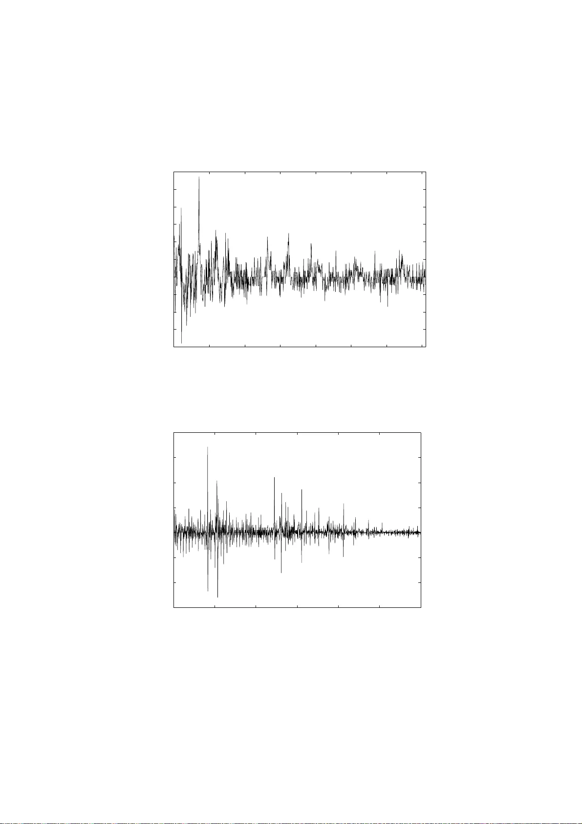
Nonp arametric sequential prediction of time series G ´ erard BIA U a, ∗ , Kevin BLEAKLEY b , L´ aszl´ o GY ¨ ORFI c and Gy¨ orgy OTTUCS ´ AK c a LST A & L PMA Univ ersit ´ e Pierre et Marie Curie – P aris VI Bo ˆ ıte 158, 175 rue du Chev aleret 75013 P aris, F rance biau@ccr.jussieu.fr b Institut de Math´ ematiques et de Mo d ´ elisation de Mon tp ellier UMR CNRS 5149 , Equipe de Probabilit´ es et Statistique Univ ersit ´ e Mon tp ellier I I, CC 051 Place Eug ` ene Bataillon, 3 4 095 Mon tp ellier Cedex 5, F rance bleakley@math.univ-montp2.fr c Departmen t of Computer Science and Information Theory Budap est Univ ersity of T ec hnology and Economics H-1117 Magy a r T ud´ osok krt. 2, Budap est, Hunga ry { gyo rfi,o ti } @szit.bme.hu Abstract Time series p rediction co vers a v ast fi eld of ev er y -d a y statistica l ap- plications in medical, environmen tal and economic domains. In this pap er w e dev elop nonp arametric p rediction strategie s b ased on the com bination of a set of “exp erts” and show the u niv ersal consistency of these strategies und er a minim um of conditions. W e p erform an in- depth analysis of real-wo rld data sets and sho w that these nonpara- metric strategies are more fl exible, f aster and generally outp erform ARMA metho d s in terms of normalized cu m u lativ e prediction error. Index T erms — Time series, sequen tial prediction, un iv ers al consis- tency , k ern el estimation, n earest n eighb or estimation, generalized lin- ear estimates. ∗ Corresp o nding author. 1 1 In tro duc tion The problem of time se ries analysis and prediction has a long and ric h history , probably dating bac k to the pioneering w ork o f Y ule in 1927 [30]. The appli- cation scop e is v ast, as time series mo deling is routinely emplo y ed across the en tire and dive rse range of applied statistics, including problems in g enetics, medical diagnoses, air p ollution forecasting, mac hine condition monitoring, financial in ve stmen ts, mark eting and econometrics. Most of the researc h activit y until the 1970s w as concerned with parametric approac hes to the problem whereb y a simple, usually linear mo del is fitted to the data (for a comprehensiv e accoun t w e refer the reader to the monograph of Bro c kwe ll and Da vies [5]). While many app ealing mat hematical prop erties of the para- metric paradigm ha v e b een established, it has b ecome clear o ve r the y ears that the limitations o f the a pproac h ma y b e rather sev ere, esse n tia lly due to o v erly rigid constrain ts which are imp osed on the processes. One of the more promising solutions to o vercome this problem has b een the extension of classic nonpa r ametric metho ds t o the time series framew ork (see for example Gy¨ orfi, H¨ ardle, Sarda and Vieu [16] and Bosq [3] for a review a nd references). In terestingly , related sc hemes hav e b een pro p osed in t he con text of se- quen tial in v estmen t strategies for financial markets . Sequen tial in ves tmen t strategies are allo wed t o use information ab out the mark et collected f r o m the past and determine at the b eginning of a training p erio d a p ortfolio, that is, a wa y to distribute the curren t capital among the a v aila ble assets. Here, the goal of the in ves tor is to maximize their we alth in the lo ng run, without kno wing the underlying distribution generating the sto c k prices. F or more information on this sub j ect, w e refer the r eader to Algo et [1], Gy¨ orfi and Sc h¨ afer [2 1], Gy¨ orfi, Lugosi and Udina [1 9], and Gy¨ orfi, Udina and W alk [22]. The presen t pa p er is dev oted to t he nonparametric pro blem of sequen tial prediction of real v alued sequence s whic h we do not require to necessarily satisfy the classical statistical assumptions for b o unded, autoregressiv e or Mark ovian pro cesses. Indeed, our goal is to sho w p ow erf ul consistency results under a strict minim um of conditions. T o fix the con text, w e supp ose that at eac h time instan t n = 1 , 2 , . . . , the statistician (also called the pr e dictor hereafter) is aske d to guess the next outc ome y n of a sequence of r eal num b ers y 1 , y 2 , . . . with know ledge of the past y n − 1 1 = ( y 1 , . . . , y n − 1 ) (where y 0 1 denotes the empty string) and the side information v ectors x n 1 = ( x 1 , . . . , x n ), where x n ∈ R d . In other w ords, adopting the p ersp ectiv e of on-line learning, the elemen ts y 0 , y 1 , y 2 , . . . and x 1 , x 2 , . . . ar e rev ealed one at a time, in order, b eginning with ( x 1 , y 0 ) , ( x 2 , y 1 ) , . . . , and the predictor’s estimate of y n at time n is based on the strings y n − 1 1 and x n 1 . F o rmally , the strategy of the 2 predictor is a sequenc e g = { g n } ∞ n =1 of forecasting functions g n : R d n × R n − 1 → R and the prediction formed at time n is just g n ( x n 1 , y n − 1 1 ). Throughout the pa p er we will supp ose that ( x 1 , y 1 ) , ( x 2 , y 2 ) , . . . are re- alizations of random v ariables ( X 1 , Y 1 ) , ( X 2 , Y 2 ) , . . . suc h tha t the pro cess { ( X n , Y n ) } ∞ −∞ is join tly stationary and ergo dic. After n time instan t s, the ( norma lize d ) cumulative squar e d pr e diction er- r or on the strings X n 1 and Y n 1 is L n ( g ) = 1 n n X t =1 g t ( X t 1 , Y t − 1 1 ) − Y t 2 . Ideally , the goa l is to mak e L n ( g ) small. There is, how ev er, a fundamen tal limit for the predictabilit y of the sequence , whic h is determined b y a result of Algo et [2]: for any prediction stra t egy g and join t ly stationary ergo dic pro cess { ( X n , Y n ) } ∞ −∞ , lim inf n →∞ L n ( g ) ≥ L ∗ almost surely , (1) where L ∗ = E n Y 0 − E Y 0 | X 0 −∞ , Y − 1 −∞ 2 o is the minimal mean squared erro r of any prediction f or the v alue of Y 0 based on the infinite pa st observ ation seque nces Y − 1 −∞ = ( . . . , Y − 2 , Y − 1 ) and X 0 −∞ = ( . . . , X − 2 , X − 1 ). Generally , w e cannot hop e t o design a strategy whose prediction error exactly ac hiev es the lo wer bound L ∗ . Rather, w e require that L n ( g ) gets arbitrarily close to L ∗ as n grow s. This giv es sense to the fo llo wing definition: Definition 1.1 A pr e diction s tr ate gy g is c a l le d universal ly c onsistent with r esp e ct to a class C of stationary and er go dic pr o c esses { ( X n , Y n ) } ∞ −∞ if for e a c h pr o c e ss in the class, lim n →∞ L n ( g ) = L ∗ almost sur ely . Th us, univ ersally consisten t strategies asymptotically ac hiev e the best p os- sible lo ss for all pro cesses in the class. Algo et [1] and Morv ai, Y ako witz and Gy¨ orfi [24] pro v ed tha t there exist univers ally consisten t strategies with resp ect to the class C of all b ounded, stationary a nd ergo dic pro cesses . Ho w- ev er, the prediction algorithms discussed in these pap ers are either v ery 3 complex or hav e an unreasonably slo w rate of conv ergence, eve n for well- b eha v ed pro cesses . Building o n the metho dology dev elop ed in recen t years for prediction of individual sequenc es (see Cesa-Bianc hi a nd Lugosi [8] for a surv ey a nd references), Gy¨ orfi and Lugosi introduced in [18] a histogram- based prediction strategy whic h is “simple” a nd ye t unive rsally consisten t with resp ect to the class C . A similar result w as also deriv ed indep enden t ly b y Nob el [25]. R o ughly speaking, bo th methods consider sev eral partition- ing estimates (called exp erts in this contex t) and com bine them at time n according to their past perfor mance. F or this, a probability distribution on the set of exp erts is generated, where a “go o d” exp ert has relativ ely large w eight, a nd the a ve rage of all experts’ predictions is tak en with resp ect to this distribution. The purp ose of this pap er is to fur t her in v estigate nonpara metric exp ert- orien ted strategies f o r un b o unded time series prediction. With this aim in mind, in Section 2.1 w e briefly recall the histogram-based prediction strategy initiated in [18], wh ic h w a s rece n tly extended to unbounded pro cesses b y Gy¨ orfi and Ottucs´ ak [20]. In Section 2.2 and 2.3 we offer tw o “more flexible” strategies, called resp ectiv ely kernel and ne ar est neighb or-b ase d prediction strategies, and state their univ ersal consistency with resp ect to the class of all (non-necessarily bounded) stationary and ergo dic processes with finite fourth momen t. In Section 2.4 we consider as an alternative a prediction strategy based o n com bining generalized linear es timates. In Section 2.5 w e use the tec hniques of the previous section to g ive a simpler prediction strategy for stationar y Gaussian ergo dic pro cesses. Extensiv e exp erimen tal results based on real- life data sets are disc ussed in Section 3, and pro ofs of the main results are giv en in Section 4. 2 Univ ers all y consiste n t pr e diction strate g ies 2.1 Histogram-based prediction strate gy In this section, w e briefly describe the histogra m- based prediction sc heme due to Gy¨ orfi and Ottucs´ ak [20] fo r unb ounde d stationary a nd ergo dic sequences. The strategy is defined at eac h time instan t as a con v ex com bination of elementary pr e d i c tors (the so-called exp erts ), where the w eigh ting co efficien ts dep end on the past performa nce of each elemen ta ry predictor. T o b e more precise, w e first define a n infinite array of exp erts h ( k, ℓ ) , k , ℓ = 1 , 2 , . . . as follo ws. Let P ℓ = { A ℓ,j , j = 1 , 2 , . . . , m ℓ } b e a sequence of finite partitions of R d , and let Q ℓ = { B ℓ,j , j = 1 , 2 , . . . , m ′ ℓ } b e a sequence of finite part it ions of 4 R . In tro duce the corresp onding quan tizers: F ℓ ( x ) = j, if x ∈ A ℓ,j and G ℓ ( y ) = j, if y ∈ B ℓ,j . T o ligh ten notation a bit, for any n and x n 1 ∈ ( R d ) n , w e write F ℓ ( x n 1 ) for the sequence F ℓ ( x 1 ) , . . . , F ℓ ( x n ) and similarly , fo r y n 1 ∈ R n w e write G ℓ ( y n 1 ) fo r the sequence G ℓ ( y 1 ) , . . . , G ℓ ( y n ). The sequence of exp erts h ( k, ℓ ) , k , ℓ = 1 , 2 , . . . is defined a s follo ws. Let J ( k, ℓ ) n b e the lo cations of the matc hes o f the last seen strings x n n − k of length k + 1 and y n − 1 n − k of length k in the past a ccording to the quantiz er with parameters k and ℓ : J ( k, ℓ ) n = k < t < n : F ℓ ( x t t − k ) = F ℓ ( x n n − k ) , G ℓ ( y t − 1 t − k ) = G ℓ ( y n − 1 n − k ) , and in tro duce the truncation f unction T a ( z ) = a if z > a ; z if | z | ≤ a ; − a if z < − a . No w define the elemen tary predictor h ( k, ℓ ) n b y h ( k, ℓ ) n ( x n 1 , y n − 1 1 ) = T n δ 1 | J ( k, ℓ ) n | X { t ∈ J ( k,ℓ ) n } y t , n > k + 1 , where 0 / 0 is defined to b e 0 a nd 0 < δ < 1 / 8 . Here and throug ho ut, for an y finite set J , the notation | J | stands for the size of J . W e note tha t t he exp ert h ( k, ℓ ) n can b e interpreted as a (t r uncated) histogram regression function estimate dra wn in ( R d ) k +1 × R k (Gy¨ orfi, Kohler, Krzy ˙ zak and W alk [1 7]). The prop osed prediction algor ithm pro ceeds with an exp onen tia l weigh t- ing av erage metho d. F ormally , let { q k ,ℓ } b e a pro babilit y distribution on the set of a ll pairs ( k , ℓ ) of p ositiv e integers suc h that f or all k and ℓ , q k ,ℓ > 0. Fix a learning pa r ameter η n > 0, and define the we igh t s w k ,ℓ,n = q k ,ℓ e − η n ( n − 1) L n − 1 ( h ( k,ℓ ) ) 5 and their norma lized v a lues p k ,ℓ,n = w k ,ℓ,n P ∞ i,j =1 w i,j,n . The prediction strategy g at time n is defined by g n ( x n 1 , y n − 1 1 ) = ∞ X k ,ℓ =1 p k ,ℓ,n h ( k, ℓ ) n ( x n 1 , y n − 1 1 ) , n = 1 , 2 , . . . It is prov ed in [20] that this sc heme is univ ersally consisten t with resp ect to the class of all (no n- necessarily b ounded) statio nary and ergo dic pro cesses with finite fourth momen t, a s stated in the f ollo wing theorem. Here and throughout the do cumen t, k · k denotes the Euclidean norm. Theorem 2.1 (Gy¨ orfi and Ot tucs´ ak [20]) Assume that (a) The se quenc e of p artitions P ℓ is neste d, that is , any c el l of P ℓ +1 is a subset of a c el l of P ℓ , ℓ = 1 , 2 , . . . ; (b) The se quenc e of p artitions Q ℓ is neste d; (c) The se quenc e of p artitions P ℓ is asymptotic al ly fi n e, i.e., if diam( A ) = sup x,y ∈ A k x − y k denotes the di a meter of a set, then for e ach spher e S c enter e d at the origin lim ℓ →∞ max j : A ℓ,j ∩ S 6 = ∅ diam( A ℓ,j ) = 0; (d) The se quenc e of p artitions Q ℓ is asymptotic al ly fine. Then, if we cho ose the le arning p ar ameter η n of the algorithm as η n = 1 √ n , the histo gr am-b as e d pr e diction scheme g defin e d ab ove is universa l ly c onsi s - tent with r esp e ct to the class of al l jointly stationary and er go dic p r o c esses such that E { Y 4 0 } < ∞ . 6 The idea of com bining a collection o f concurren t estimates was originally dev elop ed in a non-sto chastic con text for o n-line sequen tial prediction fr om deterministic sequences (see Cesa-Bianchi and Lugosi [8] for a comprehensiv e in tro duction). F ollo wing the terminology of the prediction literature, the com bination of differen t pro cedures is sometimes termed aggr e gation in the sto c ha stic contex t. The o v erall goal is alw a ys the same: use a ggregation to impro ve prediction. F or a recen t review and an up da ted list of references, see Bunea and Nob el [6] and Bunea, Tsybak o v and W egk amp [7]. 2.2 Kernel-based prediction strategies W e in tro duce in t his section a class of kernel-b ase d prediction strategies for (non-necessarily b ounded) stationary and ergo dic sequences. The main a d- v antage of this approach in con trast to the histogram-based strat egy is that it replaces t he rigid discretization of the past app earances by more flexible rules. This also often leads to faster algorithms in practical applications. T o simplify the notation, w e start with the simple “moving-windo w” sc heme, corresp onding to a unifor m ke rnel function, and treat the general case briefly later. Just lik e b efore, w e define an arra y of exp erts h ( k, ℓ ) , where k and ℓ a re positive intege rs. W e asso ciate to eac h pair ( k , ℓ ) t wo ra dii r k ,ℓ > 0 and r ′ k ,ℓ > 0 suc h tha t, for an y fixed k lim ℓ →∞ r k ,ℓ = 0 , (2) and lim ℓ →∞ r ′ k ,ℓ = 0 . (3) Finally , let the lo cation of the matche s b e J ( k, ℓ ) n = k < t < n : k x t t − k − x n n − k k ≤ r k ,ℓ , k y t − 1 t − k − y n − 1 n − k k ≤ r ′ k ,ℓ . Then the elemen ta ry exp ert h ( k, ℓ ) n at time n is defined b y h ( k, ℓ ) n ( x n 1 , y n − 1 1 ) = T min { n δ ,ℓ } P { t ∈ J ( k,ℓ ) n } y t | J ( k, ℓ ) n | ! , n > k + 1 , (4) where 0 / 0 is defined to b e 0 a nd 0 < δ < 1 / 8 . The p o ol of exp erts is mixed the same w ay as in the case of the histogram- based strategy . That is, letting { q k ,ℓ } b e a probability distribution ov er the 7 set of all pairs ( k , ℓ ) of p ositiv e in tegers suc h that q k ,ℓ > 0 for all k and ℓ , for η n > 0, we define the w eigh ts w k ,ℓ,n = q k ,ℓ e − η n ( n − 1) L n − 1 ( h ( k,ℓ ) ) together with their normalized v alues p k ,ℓ,n = w k ,ℓ,n P ∞ i,j =1 w i,j,n . (5) The general prediction sc heme g n at time n is then defined b y w eighting the exp erts according to their past p erformance and the initial distribution { q k ,ℓ } : g n ( x n 1 , y n − 1 1 ) = ∞ X k ,ℓ =1 p k ,ℓ,n h ( k, ℓ ) n ( x n 1 , y n − 1 1 ) , n = 1 , 2 , . . . Theorem 2.2 Denote by C the class of al l jointly stationary and er go dic pr o- c e s s es { ( X n , Y n ) } ∞ −∞ such that E { Y 4 0 } < ∞ . Cho ose the le arning p ar a m eter η n of the algorithm as η n = 1 √ n , and supp ose that (2) and (3) ar e v e rifie d. Then the moving-window-b ase d pr e dic tion str a te gy define d ab ove is universal ly c onsistent with r esp e ct to the class C . The pro of of Theorem 2.2 is in Section 4. This theorem ma y be extende d to a mor e g eneral class o f kernel-based strategies, as introduced in the next remark. Remark 2.1 ( General kerne l function) Define a kernel function as any m a p K : R + → R + . The kernel-b ase d str ate gy p ar al lels the moving- window scheme define d ab ove, with the o n ly d iffer enc e that in definition (4) of the elementary str ate g y, the r e gr ession function estimate is r eplac e d by h ( k, ℓ ) n ( x n 1 , y n − 1 1 ) = T min { n δ ,ℓ } P { k< t k + ¯ ℓ +1), the exp ert searche s for the ¯ ℓ nearest neigh b o rs (NN) o f the last seen observ ation x n n − k and y n − 1 n − k in the past and predicts accordingly . More precisely , let J ( k, ℓ ) n = k < t < n : ( x t t − k , y t − 1 t − k ) is among the ¯ ℓ NN of ( x n n − k , y n − 1 n − k ) in ( x k +1 1 , y k 1 ) , . . . , ( x n − 1 n − k − 1 , y n − 2 n − k − 1 ) and in tro duce the elemen tary predictor h ( k, ℓ ) n ( x n 1 , y n − 1 1 ) = T min { n δ ,ℓ } P { t ∈ J ( k,ℓ ) n } y t | J ( k, ℓ ) n | ! if the sum is non v o id, and 0 otherwise. Next, set 0 < δ < 1 8 . Finally , the exp erts are mixed as b efore: start ing from an initial proba bility distribution { q k ,ℓ } , the ag gregation sc heme is g n ( x n 1 , y n − 1 1 ) = ∞ X k ,ℓ =1 p k ,ℓ,n h ( k, ℓ ) n ( x n 1 , y n − 1 1 ) , n = 1 , 2 , . . . , where the probabilities p k ,ℓ,n are the same as in (5). 9 Theorem 2.3 Denote by C the class of al l jointly stationary and er go dic pr o c esse s { ( X n , Y n ) } ∞ −∞ such that E { Y 4 0 } < ∞ . Cho ose the p ar ameter η n of the algorithm as η n = 1 √ n , and supp ose that (6) is verifie d. Supp ose also that for e ach ve ctor s the r an d om variable k ( X k +1 1 , Y k 1 ) − s k has a c on tinuous distribution function. Then the ne ar est neighb or pr e diction str ate gy define d ab ove is universal ly c onsi s tent with r esp e ct to the class C . The pro of is a com bination of the pro of of Theorem 2.2 and the techniq ue used in [22 ]. 2.4 Generalized linear prediction strategy This section is dev oted to an alternativ e w ay of defining a univ ersal predic- tor for stationar y and ergo dic pro cesses . It is in effect an extens ion of the approac h presen ted in Gy¨ orfi and Lugosi [18] to non-necessarily b o unded pro- cesses . Once again, w e apply the metho d describ ed in the previous sections to com bine elemen tary predictors, but now w e use elemen tary predictors whic h are generalized linear predictors. More precisely , w e define an infinite array of elemen tary experts h ( k, ℓ ) , k , ℓ = 1 , 2 , . . . as follow s. Let { φ ( k ) j } ℓ j =1 b e real- v alued functions defined on ( R d ) ( k +1) × R k . The elemen tary predictor h ( k, ℓ ) n generates a prediction of form h ( k, ℓ ) n ( x n 1 , y n − 1 1 ) = T min { n δ ,ℓ } ℓ X j =1 c n,j φ ( k ) j ( x n n − k , y n − 1 n − k ) ! , where the co efficien ts c n,j are calculated according to the past observ ations x n 1 , y n − 1 1 , and 0 < δ < 1 8 . F o rmally , the co efficien ts c n,j are defined as the real num b ers which minimize the criterion n − 1 X t = k + 1 ℓ X j =1 c j φ ( k ) j ( x t t − k , y t − 1 t − k ) − y t ! 2 (7) if n > k + 1, and the all-zero vec tor o therwise. It can b e show n using a recursiv e tec hnique (see e.g., Tsypkin [29], Gy¨ orfi [15], Singer and F eder 10 [27], and Gy¨ orfi and Lugosi [18]) that the c n,j can b e calculated with small computational complexit y . The experts a re mixed via an exp onen tia l w eigh ting, whic h is defined the same w a y as earlier. Th us, the aggregated prediction sc heme is g n ( x n 1 , y n − 1 1 ) = ∞ X k ,ℓ =1 p k ,ℓ,n h ( k, ℓ ) n ( x n 1 , y n − 1 1 ) , n = 1 , 2 , . . . , where the p k ,ℓ,n are calculated according to (5). Com bining the pro of of Theorem 2 .2 and the pro of of Theorem 2 in [18] leads to the follo wing result: Theorem 2.4 Supp ose that | φ ( k ) j | ≤ 1 and, for any fi xe d k , supp ose that the set ( ℓ X j =1 c j φ ( k ) j ; ( c 1 , . . . , c ℓ ) , ℓ = 1 , 2 , . . . ) is dense in the set of c ontinuous functions of d ( k + 1) + k variables. T hen the gener alize d line ar pr e diction str ate gy define d ab o v e is universal ly c onsistent with r esp e ct to the class o f al l jointly stationary and er go dic pr o c esses such that E { Y 4 0 } < ∞ . W e g ive a sk etc h of the pro of of Theorem 2.4 in Section 4. 2.5 Prediction of Gaussian pro cesses W e consider in this section the classical problem of G a ussian t ime series prediction (cf. Bro c kw ell and Dav is [5]). In this context, parametric mo dels based on distribution assumptions and structural conditions suc h as AR( p ), MA( q ), ARMA( p , q ) and ARIMA( p , d , q ) are usually fitted to the data (cf. Gerencs ´ er and Rissanen [13], Gerencs ´ er [11, 12], G oldenshluger and Zeevi [14]). Ho we v er, in the spirit of mo dern nonparametric inference, we try to a void suc h restrictions on the pro cess structure. Th us, we only assume t ha t w e observ e a string realizatio n y n − 1 1 of a zero mean, stationary and ergo dic, Gaussian pro cess { Y n } ∞ −∞ , and try to predict y n , the v alue of the pro cess a t time n . Note that there is no side information vec tors x n 1 in this purely time series prediction f r a mew ork. It is w ell known for Gaussian time series that the b est predictor is a linear function of the past: E { Y n | Y n − 1 , Y n − 2 , . . . } = ∞ X j =1 c ∗ j Y n − j , 11 where the c ∗ j minimize the criterion E ∞ X j =1 c j Y n − j − Y n ! 2 . F o llo wing G y¨ orfi and Lugo si [18], we extend the principle o f generalized linear estimates to the prediction o f Gaussian time series b y considering the sp ecial case φ ( k ) j ( y n − 1 n − k ) = y n − j 1 { 1 ≤ j ≤ k } , i.e., ˜ h ( k ) n ( y n − 1 1 ) = k X j =1 c n,j y n − j . Once again, the co efficien ts c n,j are calculated according to the past obser- v atio ns y n − 1 1 b y minimizing the criterion: n − 1 X t = k + 1 k X j =1 c j y t − j − y t ! 2 if n > k , and the all-zero v ector otherwise. With res p ect to the com bination of elemen ta ry exp erts ˜ h ( k ) , Gy¨ orfi and Lugosi applied in [18] the so-called “doubling-t ric k”, which means that the time axis is segmen ted in to exp onentially increasing ep o chs and at the be- ginning of each ep o c h the fo recaster is reset. In this section w e prop ose a muc h simpler pro cedure whic h a v oids in particular the do ubling- tric k. T o b egin, w e set h ( k ) n ( y n − 1 1 ) = T min { n δ ,k } ˜ h ( k ) n ( y n − 1 1 ) , where 0 < δ < 1 8 , and combine these exp erts as b efo r e. Precis ely , let { q k } b e an arbitrarily probabilit y distribution o v er the p ositiv e in tegers suc h that for all k , q k > 0, and for η n > 0, define the w eights w k ,n = q k e − η n ( n − 1) L n − 1 ( h ( k ) n ) and their norma lized v a lues p k ,n = w k ,n P ∞ i =1 w i,n . 12 The prediction strategy g at time n is defined by g n ( y n − 1 1 ) = ∞ X k =1 p k ,n h ( k ) n ( y n − 1 1 ) , n = 1 , 2 , . . . By comb ining the pro of of Theorem 2.2 and Theorem 3 in [18], w e obtain the followin g result: Theorem 2.5 The line ar pr e diction str ate gy g define d ab ove is univ ersal ly c o n sistent w i th r esp e ct to the class of al l jointly stationary and er go dic zer o- me an Gaussian pr o c e sses. The f ollo wing corollary sho ws that the strategy g provide s asymptotically a go o d estimate of the r egression function in the follow ing sense: Corollary 2.1 (Gy¨ orfi and Ott ucs´ ak [20]) Under the c onditions of T he- or e m 2.5, lim n →∞ 1 n n X t =1 E { Y t | Y t − 1 1 } − g ( Y t − 1 1 ) 2 = 0 almost sur ely . Corollary 2.1 is expresse d in terms of an almost sure Ces´ aro consistency . It is an op en problem to know whether there exists a prediction rule g suc h that lim n →∞ E { Y n | Y n − 1 1 } − g ( Y n − 1 1 ) = 0 almos t surely (8) for all stationary a nd ergo dic Gaussian pro cesses . Sc h¨ af er [26] pr ov ed that, under some conditions on the time series, the consistency (8 ) holds. 3 Exp erimen tal res ults and analyses W e ev a luated the p erformance o f the histogram, mov ing-windo w k ernel, NN and Gaussian pro cess strategies on tw o real w orld data sets. F urthermore, w e compared t hese performances t o those of the standard ARMA family of metho ds on the same da t a sets. W e sho w in particular that the four metho ds presen ted in this pa p er usually p erfor m b etter than the b est ARMA results, with resp ect to three differen t criteria. The tw o real- w orld time series we in v estigated were the mon thly USA unemplo ymen t rate for Jan uary 1948 until Marc h 2 0 07 (710 p oin t s) and daily USA federal funds in terest rate fo r 12 January 2003 until 21 March 2007 (1200 p oin ts) resp ectiv ely , extracted f rom the w ebsite e c onom agic.c om . 13 0 100 200 300 400 500 600 700 −20 −15 −10 −5 0 5 10 15 20 25 30 Percentage change t Figure 1 : Monthly p ercentag e c han ge in US A unemploymen t r ate for Jan uary 1948 until Marc h 2007. 0 200 400 600 800 1000 1200 −30 −20 −10 0 10 20 30 40 t Percentage change Figure 2: Daily p ercen tage change in USA f ederal fu n ds in terest rate f or 12 Jan- uary 2003 u n til 21 Marc h 2007. 14 In o rder to remo v e first-order trends, w e transformed these time series in to time series of p er c entage change compared to the previous mon th or da y , resp ectiv ely . The resulting t ime series are show n in Figs. 1 a nd 2. Before testing the f o ur metho ds of the presen t pap er alongside the ARMA metho ds, we tested whether the resulting time series w ere trend/lev el sta- tionary using tw o standard tests, the KPSS test [23] and the PP test [1 0]. F o r b oth series using the KPSS test, w e did not reject the null h yp othesis of lev el stationarit y at p = . 01 , . 05 and . 1 respective ly , and for b oth series using the PP t est (whic h has for n ull hypothesis the existence of a unit ro ot and for alternativ e hypothesis, lev el stationarity ), the nu ll h yp ot hesis w as rejected at p = . 01 , . 05 and . 1. W e remark that this means the ARIMA( p, d, q ) f amily o f mo dels, ric her than ARMA( p, q ) is unneces sary , or equiv alently , w e need only to consider the ARIMA family ARIMA( p, 0 , q ) . As w ell as this, the Ga ussian pro cess metho d requires t he nor malit y of the data. Since the original data in b oth data sets is discretized (and not v ery finely), this meant that the data, when transformed in to p ercen tage c hanges only to ok a small num b er of fixed v alues. This had the consequenc e that directly applying standard no rmalit y tests ga v e curious results ev en when histograms of the data app eared to hav e near- p erfect Gaussian forms; ho we v er adding small amoun t s of random noise to the data allo w ed us to not system atically reject the h yp othesis of normality . Giv en eac h metho d and eac h time se ries ( y 1 , . . . , y m ) (here, m = 710 or 1200), for eac h 1 5 ≤ n ≤ m − 1 we used the data ( y 1 , . . . , y n ) to predict t he v alue o f y n +1 . W e used three criteria to measure the quality of the o ve rall set of predictions. First, as described in the presen t pa p er, w e calculated the normalized cum ulative prediction squared error L m (since w e start with n = 15 for practical reasons, this is a lmost but not exactly what ha s been called L n un til now). Secondly , we calculated L 50 m , the normalized cum ulat iv e prediction error ov er o nly the last 50 predictions of the t ime series in order to see ho w the metho d was w o r king after having learned nearly the whole time series. Thirdly , since in pra ctical situations w e may w ant to predict o nly the dir e ction of c hange, w e compared the direction ( p ositiv e or negativ e) of the last 50 predicted p oints with resp ect to each previous, kno wn p oint, to the 50 real directions. This ga ve us the criteria A 50 : the p er c entage of the dir e ction of the last 50 p oints c orr e ctly pr e dicte d . As in [19] and [22], for pr a ctical reasons w e c hose a finite grid of ex- p erts: k = 1 , . . . , K and ℓ = 1 , . . . , L for the his togram, k ernel and NN strategies, fixing K = 5 and L = 10. F o r the histogram strat- egy w e partitio ned the space in to eac h of { 2 2 , 2 3 , . . . , 2 11 } equally sized in terv als, for the ke rnel strategy w e let the radius r ′ k ,ℓ tak e the v alues r ′ k ,ℓ ∈ { . 001 , . 005 , . 01 , . 0 5 , . 1 , . 5 , 1 , 5 , 10 , 50 } and for the NN strategy w e 15 set ¯ ℓ = ℓ. F urthermore, we fixed the probabilit y distribution { q k ,ℓ } as the uniform distribution ov er the K × L exp erts. F o r the Gaussian pro cess metho d, w e simply let K = 5 and fixed the probabilit y distribution { q k } as the uniform distribution ov er the K experts. Used to compare standard metho ds with the presen t nonparametric strat- egies, the ARMA( p, q ) a lgorithm was run for all pairs ( p, q ) ∈ { 0 , 1 , 2 , 3 , 4 , 5 } 2 . The ARMA fa mily of metho ds is a com bina t io n of an autoregressiv e part AR( p ) and a mo ving-av erage part MA( q ). T ables 1 and 2 sho w the histogra m, k ernel, NN, Gaussian pro cess and ARMA results f or the unemplo ymen t and in terest rate time series resp ective ly . The three ARMA results show n in eac h table are those whic h had the b est L m , L 50 m and A 50 resp ectiv ely (sometimes t wo or more had the same A 50 , in whic h case w e c hose one of these randomly). The b est results with resp ect to eac h of the three criteria are show n in b o ld. L m L 50 m A 50 histogram 15.66 4.82 68 k ernel 15 .44 4.99 68 NN 15.40 4.97 70 Gaussian 16.35 5.02 76 ARMA(1 , 1) 16.26 5.31 72 ARMA(0 , 0) 16.68 4.86 78 ARMA(2 , 0) 16.46 5.12 78 T able 1: Results for histog ram, k ern el, NN, Gaussian pro cess an d ARMA p re- diction metho ds on the mon thly p ercenta ge c hange in USA unemploymen t rate from January 1948 un til Marc h 200 7. The thr ee ARMA results are those w hic h p erformed the b est in terms of the L m , L 50 m and A 50 criteria r esp ectiv ely . W e see via T a bles 1 and 2 that the histogram, ke rnel and NN strategies presen ted here outp erform all 36 p ossible ARMA( p, q ) mo dels (0 ≤ p, q ≤ 5) in terms of nor ma lized cum ulativ e prediction error L m , a nd that the Gaussian pro cess metho d p erfo rms similarly to the b est ARMA metho d. In terms of the L 50 m and A 50 criteria, a ll of the presen t metho ds and the b est AR MA metho d provide broadly similar r esults. F ro m a practical p oint of view, w e note also tha t the histogram, k ernel and NN metho ds also run muc h faster than a single ARMA( p, q ) trial on a standard desktop computer. F or example, the NN metho d is of the order of 10 to 100 times faster tha n an ARMA( p, q ) for a time series with ab out 1000 p oin ts, dep ending on the v alues of p and q . 16 L m L 50 m A 50 histogram 9.78 0.52 88 k ernel 9.77 0.57 86 NN 9.86 0.7 9 80 Gaussian 9.98 0.62 82 ARMA(1 , 1) 9.90 0.7 8 70 ARMA(0 , 1) 10.30 0.60 82 ARMA(3 , 0) 10.12 0.63 88 T able 2: Resu lts for histogram, k ernel, NN, Gaussian pro cess and ARMA p redic- tion metho ds on the daily p ercen tage c hange in the USA federal fund s interest rate from 12 Jan u ary 2003 un til 21 Marc h 2007 . The three ARMA r esu lts are those whic h p erform ed the b est in terms of the L m , L 50 m and A 50 criteria r esp ectiv ely . 4 Pro ofs 4.1 Pro of of T heorem 2.2 The pro of of Theorem 2.2 strongly r elies on the follow ing t wo lemmas. The first one is known as Breiman’s generalized ergo dic theorem. Lemma 4.1 (Breiman [4]) L et Z = { Z n } ∞ −∞ b e a stationary and er go dic pr o c ess. F or e ach p ositive inte ger t , let T t denote the left shift op er ator, shifting any se quenc e { . . . , z − 1 , z 0 , z 1 , . . . } by t digits to the left. L et { f t } t ≥ 1 b e a s e quenc e of r e al-v a lue d functions such that lim t →∞ f t ( Z ) = f ( Z ) almost sur ely for some function f . Supp os e that E sup t | f t ( Z ) | < ∞ . Then lim n →∞ 1 n n X t =1 f t ( T t Z ) = E { f ( Z ) } almost sur ely . Lemma 4.2 (Gy¨ orfi and Ot tucs´ ak [20]) L et h (1) , h (2) , . . . b e a se quenc e of pr e diction str ate gi e s (exp erts). L et { q k } b e a pr ob ability distribution on the set of p ositive inte gers. D enote the normalize d loss of any exp ert h = { h n } ∞ n =1 by L n ( h ) = 1 n n X t =1 L ( h t , Y t ) , wher e the loss function L is c onv ex in its fi rst ar g ume nt h t . Define w k ,n = q k e − η n ( n − 1) L n − 1 ( h ( k ) ) , 17 wher e η n > 0 i s mon o tonic al ly de c r e asing , and se t p k ,n = w k ,n P ∞ i =1 w i,n . If the pr e diction str ate g y g = { g n } ∞ n =1 is define d by g n = ∞ X k =1 p k ,n h ( k ) n , n = 1 , 2 , . . . then, for every n ≥ 1 , L n ( g ) ≤ inf k L n ( h ( k ) ) − ln q k nη n +1 + 1 2 n n X t =1 η t ∞ X k =1 p k ,t L 2 ( h ( k ) t , Y t ) . Pro of of Theorem 2.2. Because of (1 ) it is enough to sho w that lim sup n →∞ L n ( g ) ≤ L ∗ almost surely . With this in mind, w e in tro duce the follo wing notation: b E ( k, ℓ ) n ( X n 1 , Y n − 1 1 , z , s ) = P { k k + 1, where 0 / 0 is defined to b e 0, z ∈ ( R d ) k +1 and s ∈ R k . Th us, for an y h ( k, ℓ ) , w e can write h ( k, ℓ ) n ( X n 1 , Y n − 1 1 ) = T min { n δ ,ℓ } b E ( k, ℓ ) n ( X n 1 , Y n − 1 1 , X n n − k , Y n − 1 n − k ) . By a double applicatio n of t he ergo dic theorem, as n → ∞ , a lmo st surely , for a fixed z ∈ ( R d ) k +1 and s ∈ R k , w e ma y write b E ( k, ℓ ) n ( X n 1 , Y n − 1 1 , z , s ) = 1 n P { k
Original Paper
Loading high-quality paper...
Comments & Academic Discussion
Loading comments...
Leave a Comment