TRUST-TECH based Methods for Optimization and Learning

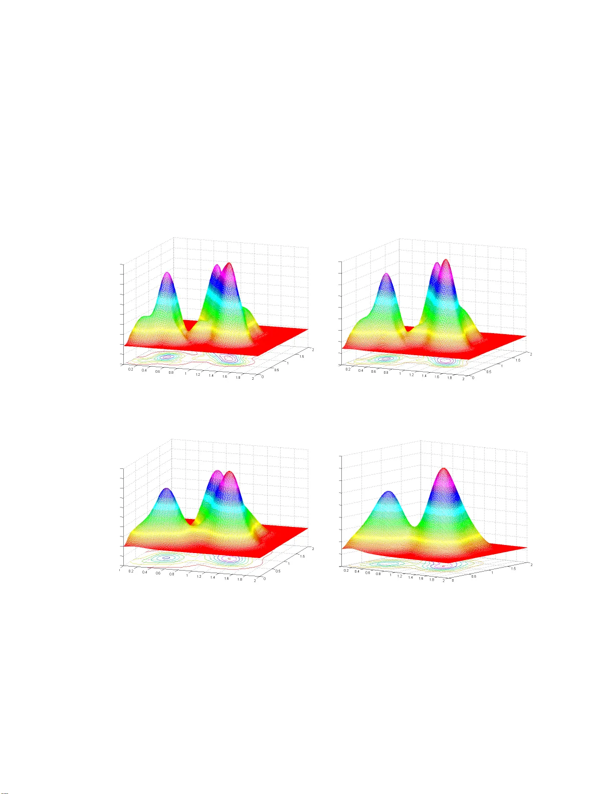
TR UST-TECH BASED METHODS F OR OPTIMIZA TION AND LEARNING A Dissertat ion Presen ted to the F aculty of the Gradua te Sc ho ol of Cor n el l Universit y in Partial F ulﬁllm en t of the Requi r ements for the Degree of Do cto r of Phil osophy b y Chandankumar Reddy Karrem Ma y 2007 c  2007 Chandank umar R eddy Kar rem ALL RIGHTS RESER VED TR UST-TECH BASED METHODS F OR OPTIMIZA TION AND LEARNING Chandankumar Reddy Karrem, Ph.D. Cornell Univ ersit y 2007 Man y problems that arise in mac hine learning domain deal with nonlinearit y and quite often demand users to obtain global optimal solutions rather than lo cal opti- mal ones. Optimization pro blems are inheren t in machine learning algorithms and hence man y metho ds in mac hine learning were inherited from the optimization lit- erature. P opularly known as the i n itialization pr oblem , the ideal set o f parameters required will signiﬁcan tly dep end on the giv en initialization v alues. The recently dev elop ed TR UST-TECH (TRa nsformation Under ST abilit y-reT a ining Equilibria CHaracterization) methodolog y s ystematically explores the subspace of the param- eters to obtain a complete set o f lo cal optimal solutions. In this thesis w ork, w e prop ose TRUST-TE CH based metho ds for solving sev eral optimizatio n and ma- c hine learning problems. TR UST-TECH explores the dynamic and geometric c har- acteristics of stabilit y b oundaries of a nonlinear dynamic al sys tem corresponding to the nonlinear f unction of inte rest. Basically , our metho d coalesces the adv a ntages of t he traditional lo cal optimizers with that of the dynamic and geometric charac- teristics of the stabilit y regions of the corresp onding nonlinear dynamical system. Tw o stages namely , the lo cal stage and the neigh b orho o d-searc h stage, are rep eated alternativ ely in the solution space to ac hiev e impro v emen t s in the qualit y of the solutions. The lo cal stage obtains the lo cal maximum of the nonlinear function and the neigh b orho o d-searc h stage helps t o escape out of the lo cal maximum b y mo v- ing tow ards the neigh b oring stability regions. Our metho ds w ere tested on b o th syn thetic and real datasets and the adv a ntages o f using this no v el framew ork a r e clearly manifested. This framework not only reduces the sensitivit y to initializa- tion, but also allow s the ﬂexibilit y for the practitioners to use v ario us global and lo cal metho ds that w ork w ell for a particular problem of inte rest. Other hierarc hi- cal sto chastic algorithms lik e ev olutionar y a lg orithms and smo o thing alg orithms are also studied and framew orks fo r com bining t hese metho ds with TRUST -TECH ha ve b een prop osed and ev a luated on sev eral test systems . BIOGRAPH ICAL SKETCH Chandan Reddy w as b orn in Jammalamadugu, Andhra Pradesh, India on May 11 , 1980. After obtaining Bache lor’s degree fro m Pondic herry Engineering College in 2001, he mov ed to the United States to pursue his higher education. He obtained his master’s degree f r om the Departmen t of Computer Science and Engineering at Michigan State Univ ersit y in August 2 003. Later, he jo ined the Departmen t of Electrical and Computer Engineering at Cornell Univ ersit y to pursue his do c- toral studies . His primary researc h inte rests are in the areas of Mac hine Learning, Data Mining, Optimization, Computational Statistics, Bioinformatics and Biomed- ical Imaging. iii Dedicated to m y paren ts iv A CKNOWLEDGEMENTS I w ould lik e to thank m y thesis advisor, Prof. Hsiao-Do ng Chiang, without whose guidance and in v olv emen t this w ork w ould not hav e been p ossible. His enth usiasm and inspiration w ere extremely helpful in succes sfully pursuing this researc h w o rk. I would also lik e to thank m y committee mem b er Prof. John Hop croft for his encouragemen t and useful discussions. I am g rateful t o Dr. P eter D o ersc h uk for serving o n m y thesis committee. Sp ecial thanks to Dr. Bala Ra jara t na m for his help with a few statistical w orks related to m y thesis. I am deeply indebted to m y father, who w as m y main inspiration for pursuing graduate studies and c ho o sing to ha v e an academic career. Ne edless to sa y I had plen ty of gr eat discussions and fun with many p eople in the departmen t including Jeng-Heui, W arut, Choi, Seunghee , Siv a, Bha vin, W esley , Jay and Huach en. I w as also for t una t e t o hav e a go o d compan y at Cornell who hav e k ept my spirits up and my life in teresting: Manpree t, P alla vi, Sudha, R a ju, Kumar, Mahesh, P ank a j, Deepak, Pradeep, Ajay and Shobhit. A special tha nks to the graduate secretaries for taking care of coun tless n um b ers of things without an y hitc h. Last a nd the most imp o r t an t, m y deep est gratitude go es to m y dear mother f o r her lo ve, a nd for making me the p erson I a m. v T A BLE OF CONTE NTS 1 In t ro duction 1 1.1 Mac hine L ear ning . . . . . . . . . . . . . . . . . . . . . . . . . . . . . 1 1.2 Optimization Metho ds . . . . . . . . . . . . . . . . . . . . . . . . . . 3 1.3 Motiv ation for this Thesis . . . . . . . . . . . . . . . . . . . . . . . . 6 1.4 Con tributions of this Thesis . . . . . . . . . . . . . . . . . . . . . . . 8 1.5 Organization of this Thesis . . . . . . . . . . . . . . . . . . . . . . . . 9 2 Finding Saddle Poin ts on Poten tial Energy Surfaces 11 2.1 In tro duction . . . . . . . . . . . . . . . . . . . . . . . . . . . . . . . . 11 2.2 Relev an t Bac kgro und . . . . . . . . . . . . . . . . . . . . . . . . . . . 14 2.3 Theoretical Bac kground . . . . . . . . . . . . . . . . . . . . . . . . . 15 2.4 A Stability Boundary ba sed Metho d . . . . . . . . . . . . . . . . . . 21 2.5 Implemen tation Iss ues . . . . . . . . . . . . . . . . . . . . . . . . . . 25 2.6 Exp erimental Results . . . . . . . . . . . . . . . . . . . . . . . . . . . 30 2.6.1 T est Case 1 : Tw o-dimensional P otential Energy Surface . . . . 30 2.6.2 T est Case 2 : Three-dimensional symmetric systems . . . . . . 33 2.6.3 T est Case 3 : Higher Dimensional Systems . . . . . . . . . . . 36 2.6.4 Sp ecial Cases : Ec khardt surface . . . . . . . . . . . . . . . . 40 2.7 Discussion . . . . . . . . . . . . . . . . . . . . . . . . . . . . . . . . . 43 3 TRUST-TECH based Exp ectation Maximization for Learning Mix- ture Mo dels 47 3.1 Relev an t Bac kgro und . . . . . . . . . . . . . . . . . . . . . . . . . . . 49 3.2 Preliminaries . . . . . . . . . . . . . . . . . . . . . . . . . . . . . . . 51 3.2.1 Mixture Mo dels . . . . . . . . . . . . . . . . . . . . . . . . . . 52 vi 3.2.2 Exp ectatio n Maximization . . . . . . . . . . . . . . . . . . . . 53 3.2.3 EM for GMMs . . . . . . . . . . . . . . . . . . . . . . . . . . 55 3.2.4 Nonlinear T r a nsformation . . . . . . . . . . . . . . . . . . . . 56 3.3 TR UST-TECH based Expectation Maximization . . . . . . . . . . . . 58 3.4 Implemen tation Details . . . . . . . . . . . . . . . . . . . . . . . . . . 6 0 3.5 Results and Discussion . . . . . . . . . . . . . . . . . . . . . . . . . . 62 3.5.1 Syn thetic D atasets . . . . . . . . . . . . . . . . . . . . . . . . 64 3.5.2 Real D atasets . . . . . . . . . . . . . . . . . . . . . . . . . . . 65 3.5.3 Discussion . . . . . . . . . . . . . . . . . . . . . . . . . . . . . 66 4 Motif Reﬁnemen t using Neighborho o d P roﬁle Searc h 71 4.1 Relev an t Bac kgro und . . . . . . . . . . . . . . . . . . . . . . . . . . . 73 4.2 Preliminaries . . . . . . . . . . . . . . . . . . . . . . . . . . . . . . . 75 4.2.1 Problem F orm ulation . . . . . . . . . . . . . . . . . . . . . . . 7 5 4.2.2 Dynamical Systems for the Scoring F unction . . . . . . . . . . 78 4.3 Neigh b orho o d Proﬁle Search . . . . . . . . . . . . . . . . . . . . . . . 8 0 4.4 Implemen tation Details . . . . . . . . . . . . . . . . . . . . . . . . . . 8 5 4.5 Exp erimental Results . . . . . . . . . . . . . . . . . . . . . . . . . . . 88 4.5.1 Syn thetic D atasets . . . . . . . . . . . . . . . . . . . . . . . . 89 4.5.2 Real D atasets . . . . . . . . . . . . . . . . . . . . . . . . . . . 93 5 Comp onen t-wise Smo othing for Learning Mixture Mo dels 96 5.1 Ov erview . . . . . . . . . . . . . . . . . . . . . . . . . . . . . . . . . . 96 5.2 Relev an t Bac kgro und . . . . . . . . . . . . . . . . . . . . . . . . . . . 97 5.3 Preliminaries . . . . . . . . . . . . . . . . . . . . . . . . . . . . . . . 101 5.4 Smo othing Log-Lik eliho o d Surfa ce . . . . . . . . . . . . . . . . . . . . 103 5.4.1 Kernel P arameters . . . . . . . . . . . . . . . . . . . . . . . . 105 vii 5.4.2 EM Updates . . . . . . . . . . . . . . . . . . . . . . . . . . . . 106 5.5 Algorithm and its implemen tation . . . . . . . . . . . . . . . . . . . . 106 5.6 Results and Discussion . . . . . . . . . . . . . . . . . . . . . . . . . . 109 5.6.1 Reduction in t he num b er of lo cal maxima . . . . . . . . . . . 112 5.6.2 Smo othing for Initialization . . . . . . . . . . . . . . . . . . . 112 6 TRUST-TECH based Neural Netw ork T raining 121 6.1 Ov erview . . . . . . . . . . . . . . . . . . . . . . . . . . . . . . . . . . 121 6.2 Relev an t Bac kgro und . . . . . . . . . . . . . . . . . . . . . . . . . . . 124 6.3 T raining Neural Net works . . . . . . . . . . . . . . . . . . . . . . . . 128 6.4 Problem T ransformat io n . . . . . . . . . . . . . . . . . . . . . . . . . 131 6.5 TR UST-TECH based T raining . . . . . . . . . . . . . . . . . . . . . . 132 6.6 Implemen tation Details . . . . . . . . . . . . . . . . . . . . . . . . . . 136 6.6.1 Arc hitecture and Lo cal Methods . . . . . . . . . . . . . . . . . 136 6.6.2 Initialization Sc hemes . . . . . . . . . . . . . . . . . . . . . . 137 6.6.3 TR UST-TECH . . . . . . . . . . . . . . . . . . . . . . . . . . 137 6.7 Exp erimental Results . . . . . . . . . . . . . . . . . . . . . . . . . . . 139 6.7.1 Benc hmark D atasets . . . . . . . . . . . . . . . . . . . . . . . 139 6.7.2 Error Estimation . . . . . . . . . . . . . . . . . . . . . . . . . 141 6.7.3 Classiﬁcation Accuracy . . . . . . . . . . . . . . . . . . . . . . 142 6.7.4 Visualization . . . . . . . . . . . . . . . . . . . . . . . . . . . 144 7 E v olutionary TRUST- TECH 146 7.1 Ov erview . . . . . . . . . . . . . . . . . . . . . . . . . . . . . . . . . . 146 7.2 V ariants of Ev olutiona ry Algorithms . . . . . . . . . . . . . . . . . . 148 7.3 Ev olutio nary TR UST-TECH Algorithm . . . . . . . . . . . . . . . . . 151 7.4 Exp erimental Results . . . . . . . . . . . . . . . . . . . . . . . . . . . 154 viii 7.5 P a rallel Ev olutiona ry TR UST-TECH . . . . . . . . . . . . . . . . . . 155 8 Conclusion and F uture W ork 156 8.1 Conclusion . . . . . . . . . . . . . . . . . . . . . . . . . . . . . . . . . 156 8.2 F uture W o rk . . . . . . . . . . . . . . . . . . . . . . . . . . . . . . . . 159 Bibliograph y 162 ix LIST OF FIGURES 1.1 (a) Sup ervised learning with data p oin ts from tw o diﬀeren t classes separated b y a h yp erplane represen ted using a dashed line. (b) Un- sup ervised Learning or data clustering - t w o w ell separated clusters. 3 1.2 Diﬀeren t optimization metho ds. . . . . . . . . . . . . . . . . . . . . . 4 1.3 V arious stages of TR UST-TECH (a) The dark regions indicate the promising subspaces. (b) The dots indicate the lo cal optimal solu- tions a nd the dott ed arrows indicate t he con v ergence of lo cal opti- mization metho d from a given initial p oint. . . . . . . . . . . . . . . 7 1.4 Organization chart o f this thesis. The main contributions are in the areas of optimizatio n and learning. . . . . . . . . . . . . . . . . . . . 10 2.1 The surface and con tour plots of a t w o-dimensional energy function. A saddle p oint ( x d ) is lo cated b etw een t wo lo cal minima ( x 1 s and x 2 s ). x 1 m and x 2 m are tw o lo cal maxima lo cated in the orthog o nal direction. 13 2.2 Phase pot r ait of a gradien t system. The solid lines with solid arro ws represen t the basin b oundary . ∂ A p ( x 1 s ) = S 3 i =1 W s ( x i d ). The lo cal minima x 1 s and x 2 s corresp ond to the stable equilibrium p oin ts of the gradien t system. The saddle p oint ( x 1 d ) correspo nds to the dynamic decomp osition p oint that connects the t wo stable equilibrium p oints. 18 x 2.3 Con tour plot of a 2-D LEPS p otential (describ ed in a pp endix-A). Eac h line represen ts the v alues of a constant pot en t ia l. A and B are the t w o lo cal minima. D D P is the dynamic decomp o sition p oin t to b e computed. The searc h direction is the direction of the v ector joining AB. The exit p oin t ( X ex ) is obtained by ﬁnding the p eak of the function v alue along this v ector. The do tted line indicates the stabilit y b oundary . The dashed line indicates the searc h direction. . 22 2.4 Illustration of the step 3 of our alg orithm. m 1 is in tegrated till m ′ 1 is reac hed a nd traced bac k along the v ector m ′ 1 B t o get m 2 , and so on. m n are the n exit p oin ts on the stability b oundary . The n th p oin t is the Minim um Gradien t Poin t where the magnitude of the gradien t ( G M ) is the minim um amongst all the computed gradien t v alues along the stability b o undary ( X ex , m 2 , m 3 .. m n ). D DP is the dynamic decompo sition p oint. . . . . . . . . . . . . . . . . . . . . . . 24 2.5 The plot of the function v alue alo ng t he v ector AB . The curv e monotonically increases starting f rom A and then decreases till it reac hes B . X ex is the exit p oin t where the function attains its peak v alue. a 1 , a 2 , ... a 9 are the interv a l p oin ts. The mark ed circles indicate that the function has b een ev aluated at these p oints. The empt y circles indicate the p oin ts where the function is ye t to b e ev aluated. . . . . . . . . . . . . . . . . . . . . . . . . . . . . . . . . . 26 2.6 The in terv al p oint a 5 can b e presen t either to the left or to the righ t of t he p eak. When a 6 is reac hed, the golden section searc h metho d is in vok ed with a 6 and a 4 as the interv a l. . . . . . . . . . . . . . . . . 2 7 xi 2.7 Tw o dimensional con tour plo t of the p oten tial energy surface cor- resp onding to the m uller-brown function described in Eq. (2 .12). A,B and C ar e stable equilibrium p oin ts and DDP1,DD P2 are t w o dynamic decomp osition p o in ts. The dashed lines indicate the ini- tial searc h direction. The dots indicate the results of the stabilit y b oundary following pro cedure. These p oin ts are the p oints on the stabilit y b oundary that reac h the MGP . . . . . . . . . . . . . . . . . 31 2.8 The gradien t curv e corresp onding to the v ar ious p oin ts obtained from the stabilit y b oundar y follow ing pro cedure. The graph sho ws that the magnitude of the gradien t slo wly increases in the initial phases and then starts to reduce. The highligh ted p oin t corresponds to the gradien t at the MGP . . . . . . . . . . . . . . . . . . . . . . . . . . . 33 2.9 Characteristic curv es of Lennard-Jones p o t en t ia l and the Morse p o- ten tial with all parameters set to unit y . Solid line represen ts Lennard- Jones p oten tial (2 .1 3) and the dashed line represen ts the Morse p o- ten tial (2.15). . . . . . . . . . . . . . . . . . . . . . . . . . . . . . . . 35 2.10 T op view of the surfa ce and the sev en a tom island on the surface of an FCC crystal. The shading indicates the heigh t of the atoms. . . . 37 2.11 Some sample conﬁgurations of the heptamer island on the surface of the F CC crystal. F ir st ro w- saddle p oin ts conﬁgurations. Second ro w- other lo cal minim um energy conﬁguratio ns corresp onding to t he ab ov e saddle p o in t conﬁgurations. . . . . . . . . . . . . . . . . . . . 39 2.12 The gradient curv e obtained in o ne of the higher dimensional test cases. MGP indicates the minim um gra dien t p oint where the mag- nitude of the g radien t reac hes the minimum v alue. This p oin t is used as a initial guess for a lo cal optimization method to obtain DDP . . . 39 xii 2.13 Tw o dimensional contour plot of the p oten tial energy surface of the Ec khardt energy function describ ed on Eq. (2.18). A and B are stable equilibrium p oin ts and DDP1,D DP2 a r e tw o dynamic decom- p osition p oints. M is a source. The dots corresp o nd to t he p oints on the stability b oundary during the stability b oundary following pro cedure. . . . . . . . . . . . . . . . . . . . . . . . . . . . . . . . . 41 2.14 Gradien t curv e corresp onding to the v arious p oin ts along the stabilit y b oundary on the Ec khardt surface. . . . . . . . . . . . . . . . . . . . 42 3.1 Data consisting of three Gaussian comp onen t s with diﬀerent mean and v ariance v alues. Not e that eac h data p oin t do esn’t ha v e a hard mem b ership that it b elongs to only o ne comp onent. Most of the p oin ts in the ﬁrst comp onen t will hav e high proba bility with whic h they b elong to it. In this case, the o t her comp onen ts do not hav e m uc h inﬂuence. Componen ts 2 and 3 data p oints are no t clearly separated. The problem of lear ning mixture mo dels in v olv es esti- mating the parameters of the G aussian components a nd ﬁnding the probabilities with whic h each data sample b elongs to the comp onen t . 49 3.2 V arious stages of o ur alg orithm in (a ) P arameter space - the solid lines indicate the practical stabilit y b o undary . P oints highligh ted on the stability b oundary are the decomp osition p oints . The dotted arro ws indicate the con v ergence of the EM algor it hm. The dashed lines indicate t he neigh b o r ho o d-search stag e. x 1 and x 2 are the exit p oin ts on the practical stabilit y b o undar y (b) Diﬀeren t p oin ts in the function space and their corresponding log-lik eliho o d function v alues. 58 xiii 3.3 P a rameter estimates a t v a rious stages of our a lgorithm on the three comp onen t Gaussian mixture mo del (a) P o or ra ndo m initial guess (b) Lo cal maxim um obtained after applying EM algorithm with the p o or initial guess (c) Exit p oin t obtained b y our algo r it hm (d) The ﬁnal solution obtained by applying the EM algorithm using the exit p oin t as the initial guess. . . . . . . . . . . . . . . . . . . . . . . . . 63 3.4 Graph sho wing lik eliho o d vs Ev a luations. A corr esp o nds to the o rig- inal lo cal maxim um (L=-3235 .0 ). B corresp onds to the exit p oint (L=-3676 .1 ). C corresp onds to the new initial p oint (L=-365 7 .3) after mo ving out b y ‘ ǫ ’. D corresp onds to the new lo cal ma ximum (L=-3078 .7 ). . . . . . . . . . . . . . . . . . . . . . . . . . . . . . . . 64 4.1 Syn thetic DNA sequences containing some instance of the pat t ern ‘CCGA TT A CCGA’ with a maxim um n um b er of 2 m utations. The motifs in eac h sequence are highligh ted in the b o x. W e hav e a (11,2) motif where 11 is the length of the motif and 2 is the n um b er of m utations allo w ed. . . . . . . . . . . . . . . . . . . . . . . . . . . . . 7 2 4.2 Diagram illustrates the TR UST-TECH metho d of escaping from the original solution ( A ) to the neighborho o d lo cal optimal solutions ( a 1 i ) through the corresp onding exit p oints ( e 1 i ). The dotted lines indicate the lo cal con vergenc e of the EM algorithm. . . . . . . . . . . 82 4.3 A summary of escaping out o f the lo cal optim um to the neighborho o d lo cal optimum. Observ e the corresp onding trend of the a lignmen t score at each step. . . . . . . . . . . . . . . . . . . . . . . . . . . . . 83 xiv 4.4 2-D illustration of ﬁrst tier impro v emen t s in a 3 l dimensional ob j ec- tiv e function. The original lo cal maxim um has a score of 163.3 75. The v arious Tier-1 solutions are plotted and the one with highest score (167.81) is chos en. . . . . . . . . . . . . . . . . . . . . . . . . . 88 4.5 The av erage scores with the corresponding ﬁrst tier and second tier impro v emen ts on syn thetic data using the random starts with TR UST- TECH approac h with diﬀeren t ( l,d ) motifs. . . . . . . . . . . . . . . 92 4.6 The av erage scores with the corresponding ﬁrst tier and second tier impro v emen ts on sy nthe tic data using the Random Pro jection with TR UST-TECH approac h with diﬀeren t ( l , d ) mot if s. . . . . . . . . . . 92 5.1 Blo c k diag ram of the traditional approa c h and the smo othing approac h. 99 5.2 Smo othing a nonlinear surface at diﬀeren t lev els. T racing the global maxima (A, B and C) at diﬀerent levels . . . . . . . . . . . . . . . . . 100 5.3 Diﬀeren t con volution ke rnels (a) T riangula r function (b) Step func- tion and (c) Gaussian function . . . . . . . . . . . . . . . . . . . . . 102 5.4 The eﬀects of smo othing a Ga ussian densit y function with a Gaussian k ernel. . . . . . . . . . . . . . . . . . . . . . . . . . . . . . . . . . . . 103 5.5 Blo c k Diagra m of the smo othing approach. Smo oth lik eliho o d sur- face is obtained by con volv ing the original likelihoo d surface with a con v olution k ernel whic h is c hosen to b e a Gaussian k ernel in our case. 105 5.6 Flo w c hart of the smo othing algorithm . . . . . . . . . . . . . . . . . 107 5.7 T rue mixture of the three Gaussian comp onen ts with 900 samples. . 109 5.8 T rue mixtures of the more complicated ov erlapping Gaussian case with 1000 samples. . . . . . . . . . . . . . . . . . . . . . . . . . . . . 110 xv 5.9 V arious stag es during the smo othing pro cess. (a) The origina l log- lik eliho o d surface whic h is v ery rugg ed (b)- (c) In termediate smo othened surfaces (d) Final smo o thened surface with only t w o lo cal maxima. 111 5.10 Reduction in the n um b er of lo cal maxima for v arious datasets. . . . 113 6.1 The Arc hitecture of MLP with single hidden la y er ha ving k hidden no des and the output lay er having a single output no de. x 1 , x 2 , ..., x n is an n- dimensional input feature vector. w ij are the w eights and b 1 , b 2 , ..., b k are the biases for these k no des. The a ctiv ation function for the hidden no des is sigmoidal and for the o ut put no de is linear. . 122 6.2 Comparison b et wee n the tw o framew orks (a) T raditional approac h and (b) TRUST -TECH based approac h. The main diﬀerence is the inclusion of the stabilit y region ba sed neigh b or ho o d- searc h stage that can explore the neighborho o d solutions. . . . . . . . . . . . . . . . . 123 6.3 Blo c k Diagram of the TRUST -TECH based training metho d. . . . . 127 6.4 Flo w c ha rt of our metho d . . . . . . . . . . . . . . . . . . . . . . . . 133 6.5 Diagram Illustrating tw o tier exit p oint strategy . The ‘A*’ represen ts the initial guess. Dotted arrows repres en t the conv ergence o f the lo cal solv er. Solid arrow s represen t t he gradien t ascen t linear searc hes along eigen v ector directions. ‘X’ indicates a new initial condition in the neighboring stabilit y region. M repres en ts the lo cal minim um obtained b y applying lo cal metho ds from ’X’. A 1 i indicates Tier-1 lo cal minima. e 1 i are the exit p oin ts b et w een M and A 1 i . Similarly , A 2 j and e 2 j are the sec ond-tier lo cal minima and their corr espo nding exit po ints respectiv ely . . . . . . . . . . . . . . . . . . . . . . . . . . 135 xvi 6.6 Spider w eb diag r ams sho wing the tier- 1 and tier-2 impro v emen ts us- ing TR UST-TECH metho d on v arious b enc hmark da t a sets. The basis t w o axes are c ho sen arbitrarily and t he v ertical a xis represen ts the impro ve men ts in the classiﬁer accuracy . The distances b et w een eac h tier are normalized to unit y . . . . . . . . . . . . . . . . . . . . 145 7.1 T op olog y of the nonlinear surface discussed in t he introduction c hap- ter. The initial p oint o bta ined after the r ecombination is ‘s’. The original concept of m utations will randomly p erturb the p oint in the parameter space and obtain diﬀerent p oints ( s 1 , s 2 and s 3 ). Tw o diﬀeren t ev olutionary mo dels (a) Lo cal reﬁnemen t strategy where the local optimization metho d is applied with ‘s’ as initial guess to obtain ‘A’. (b) Ev olutionary TR UST-TECH metho dology where the surrounding solutions are explored systematically af ter the recom bi- nation. . . . . . . . . . . . . . . . . . . . . . . . . . . . . . . . . . . 152 xvii LIST OF T ABLES 2.1 Stable equilibrium p oints and DDPs fo r the Muller-Bro wn Surf ace described in Eq. (2.12). . . . . . . . . . . . . . . . . . . . . . . . . . 32 2.2 Stable equilibrium p oints and dynamic decompo sition p oin ts for the Muller-Bro wn Surface described in Eq. (2.12). . . . . . . . . . . . . . 33 2.3 Stable equilibrium p oints and dynamic decompo sition p oin ts for the three atom Lennard Jones Cluster described in Eq. ( 2.13). . . . . . . 36 2.4 Results of our algorithm on a heptamer island ov er the F CC crystal. The num b er of force ev aluations made to compute the MGP is giv en in the la st column. . . . . . . . . . . . . . . . . . . . . . . . . . . . 40 2.5 Stable equilibrium p oints and dynamic decompo sition p oin ts for the Ec khardt Surface. . . . . . . . . . . . . . . . . . . . . . . . . . . . . 4 2 3.1 Description of the Notations used . . . . . . . . . . . . . . . . . . . . 52 3.2 P erf o rmance of TR UST-TECH-EM algorithm on an a v erage of 100 runs on v arious syn thetic and real datasets compared with random start EM a lg orithm . . . . . . . . . . . . . . . . . . . . . . . . . . . 65 3.3 Comparison of TR UST-TECH-EM with other methods . . . . . . . . 66 3.4 Num b er of iterations tak en for the con ve rgence of the b est solution. 67 4.1 A coun t of n ucleotides A, T , G, C at eac h p osition k = 1 ..l in all the sequence s of the data set. k = 0 denotes the bac kground coun t. . . . 76 4.2 A count of n ucleotides j ∈ { A, T , G, C } at eac h p osition k = 1 ..l in all the sequ ences of the data set. C k is the k th n ucleotide of the consensus pattern whic h represen ts the n ucleotide with the highest v alue in that column. L et the consensus pattern b e GA CT...G and b j b e the bac kground. . . . . . . . . . . . . . . . . . . . . . . . . . . 79 xviii 4.3 The consensus pa t terns and their correspo nding scores of the original lo cal optimal solution obtained from m ultiple random star t s on the syn thetic data. The best ﬁrst tier and se cond tier optimal patterns and their corresponding scores are also r ep orted. . . . . . . . . . . . 9 1 4.4 The results of p erformance co eﬃcien t with m = 1 on syn thetically generated sequences . The IC scores are not normalized and the p er- fect score is 20 since there are 20 sequenc es. . . . . . . . . . . . . . 93 4.5 Results of TR UST-TECH metho d on biolog ical samples. The real motifs were obta ined in all the six cases using the TRUST-TE CH framew ork. . . . . . . . . . . . . . . . . . . . . . . . . . . . . . . . . 94 5.1 Comparison of smo othing algorithm with the random starts. Mean and standard deviations across 100 random starts are rep orted. . . . 1 14 6.1 Description of the notations used . . . . . . . . . . . . . . . . . . . . 129 6.2 Summary of Benc hmark Data sets. . . . . . . . . . . . . . . . . . . . 141 6.3 P ercentage improv emen ts in the classiﬁcation accuracies ov er t he training and test data using TRUS T-TECH with m ult iple random restarts. . . . . . . . . . . . . . . . . . . . . . . . . . . . . . . . . . 143 6.4 P ercentage improv emen ts in the classiﬁcation accuracies ov er t he training and test data using TRUS T-TECH with MA TLAB initial- ization. . . . . . . . . . . . . . . . . . . . . . . . . . . . . . . . . . . 143 7.1 Results of Evolutionary TR UST-TECH mo del . . . . . . . . . . . . 154 xix Chapter 1 In tro duction The problem of ﬁnding a global optimal solution arise in many disciplines ranging from science to engineering. In real w orld applications, m ulti-dimensional ob jec- tiv e functions usually con tain a large n umber o f lo cal optimal solutions. Obtaining a g lobal optimal solution is of primary imp ortance in these a pplicatio ns and is a v ery c hallenging problem. Some examples of these applications are : molecular conﬁrmation prediction [22], VLSI design in micro electronics [95], resource allo ca- tion problems [41], design of wireless net w o rks [69], ﬁnancial decision making [87], structural engineering [58] and parameter estimation problems [53]. In this thesis, the primary fo cus is on the parameter estimation pr o blems that a rise in the ﬁeld of mac hine learning. 1.1 Mac hine Learning Mac hine learning algorithms can b e broa dly classiﬁed in to tw o catego ries [44]: (i) Sup ervised learning and (ii) Unsup ervised learning. The primary go a l in sup e rv ise d le arning is to learn a mapping from x to y giv en a training data set whic h consists of pairs ( x i , y i ), where x i ∈ X are the data p oints and y i ∈ Y are the lab els (or targets). A standard assumption is that the pairs ( x i , y i ) are sampled i.i.d. from some distribution. If y tak es v alues in a ﬁnite set (discrete v alues) then it is a clas- siﬁcation problem and if it take s v alues in a con t in uous space, then it is a regression problem. Supp ort v ector mac hines [21], a r tiﬁcial neural net w orks [68] and bo osting [61] are the most p opular algorithms for supervised learning. All these alg orithms will construct a classiﬁcation (o r regression) mo del ba sed on certain training data a v ailable. Usually , the eﬀectiv eness of any algorithm is ev aluated using testing data 1 whic h is separate from the training data. In this thesis, w e will primarily fo cus on artiﬁcial neur al ne twork s a nd estimating the parameters of its mo del. Constructing a mo del using artiﬁcial neural netw ork inv olv es estimating the parameters of the mo del that can eﬀectiv ely exploit the p otential of the mo del. These parameters are usually obtained by ﬁnding the global minim um on the error surface. More details on t r a ining neural net w orks will b e presen ted in Chapter 6. Unsup ervise d le arning , on the other hand, will train mo dels using only the data- p oin ts without the target v alues. In simple terms, o nly x v alues are a v ailable without y v alues. Problems lik e outlier detection, densit y estimation, data clustering and noise remo v al f a ll under this categor y . Data clustering is one of the widely studie d unsup ervised learning topics [82]. D ensit y estimation is a more generalized notion of data clustering. It in volv es in estimating and understanding and the underlyin g distribution of the data. Applications of densit y estimation include trend analysis and data compression. Ty pically , one w ould lik e t o estimate the parameters of a mo del that consists of m ultiple comp onen ts o f v arying densities. More details on these mixture mo dels and the use of exp ectation maximiz ation (EM) algorithm for parameter estimation of these mo dels will b e presen ted in Chapter 3. Fig. 1.1 sho ws the sup ervised and unsup ervised learning scenarios. In sup ervised learning, the main go a l is to tra in a mo del suc h that a ﬁnal target class can b e estimated for a new (unseen) data p oint. In a simple binary classiﬁc ation problem, a h yp erplane (indicated by a dashed line) separates b oth t he classes. In clustering problems, the main goal is to form gro upings of the dat a and obtain an y in teresting structure (or patterns) in the data (see Fig. 1.1(b) ) . In b oth the mo dels men tioned ab ov e (neural net w orks and mixture mo dels), estimating the parameters corresp ond to o btaining a g lobal optimal solution on a highly nonlinear surface. The surface can b e generated based on a function that 2 (a) supervised Learning (b) Unsupervised Lear ning Figure 1.1: (a) Sup ervised learning with dat a p oints from t w o diﬀeren t classes sep- arated b y a h yp erplane represen ted using a dashed line. (b) Unsup ervised Learning or data clustering - t w o w ell separated clusters. migh t represen t the error in the training data o r the lik eliho o d of the data giv en the mo del. W e will no w introduce diﬀeren t categories of the nonlinear optimization metho ds studied in the literature. 1.2 Optimization Metho d s Optimization metho ds can b e bro adly classiﬁed in to tw o catego r ies: glob al meth- o ds and lo c al metho ds . Global metho ds explore the en tire searc h space and obtain promising regions t ha t hav e a higher proba bilit y of ﬁnding a global optimal solutio n. They can b e either deterministic or sto c ha stic in nature dep ending on the usage of some random comp onent in the algorithm [78]. Deterministic global metho ds include branc h and b ound [79], homotop y ba sed [59 ], interv al analysis [66] and tra jectory- based [39]. These metho ds are a lso kno wn a s exact metho ds. Sto c hastic g lo bal metho ds include tec hniques suc h as ev olutionary alg orithms [3], sim ula ted anneal- ing [88], tabu searc h [5 4] and an t colon y optimization [42] whic h can g iv e a symptotic guaran tees o f ﬁnding the global optimal solution. Man y heuristic searc h a lgorithms can b e incorp orated in to these sto chastic metho ds to improv e the p erfor mance of the algorithm in terms of qualit y of the solutio n and the sp eed of conv ergence. 3 Figure 1.2: Diﬀerent optimization metho ds. 4 Usually , lo cal metho ds are deterministic in nature and can be group ed into tw o categories: gr adient b ase d and non-g r adient b as e d metho ds . 1. Gr adient b ase d metho ds can b e further classiﬁed into (i) Line searc h meth- o ds and (ii) T rust-r egio n methods. Line searc h algorit hms usually select some descen t direction (based on the gradien t information) and minimize the func- tion v alue a long the chosen direction. This pro cess is rep eated un til a lo cal minim um is reached. The most p o pular line search algorithms include steep- est descen t [116], conjuga te gradien t [2] a nd Newton-Raphson metho d [110]. T rust region metho ds [2 4, 96], on the other hand, mak e an assumption ab out the nonlinear surface locally and do not use an y form of line searc h. T ypically , they assume the surface to b e a simple quadratic mo del suc h that the mini- m um can b e lo cated directly if the mo del assumption is g o o d whic h usually happ ens when the initial g uess is close to the lo cal minim um. If the mo del assumption is not accurate, then gradien t infor ma t io n is used to guide the initial guess and after a certain p erio d the mo del assumption is made ag ain. 2. In contrast to the ab o v e men tioned gradien t based metho ds, non-gr adien t b ase d metho ds do not use any gradien t information. Usually , these metho ds rely on a particular fo rm of the nonlinear function a nd ensure that a chose n it- erativ e parameter up dating sc heme results in the decrease of the function v alue [28]. F or densit y estimation problems using ma ximum lik eliho o d function, a p opular class of iterative parameter estimation metho ds is the Exp ectation Maximization (EM) algo r it hm whic h conv erges to the maxim um lik eliho o d estimate of t he mixture parameters lo cally [37, 123]. 5 1.3 Motiv ation for this T hesis Finding the global optimal solution of a function is a lot more t edious and c halleng- ing for man y problems. The task of ﬁnding suc h a solution is quite complex and increases rapidly with the dimensionality of the problem. T ypically , the problem of ﬁnding t he global optimal solution is solv ed in a hierarc hical manner. Iden tifying some pro mising regions in a searc h space is relatively easier using certain g lobal metho ds (suc h as genetic algorithms and simulated annealing) av ailable in t he lit- erature. Ho wev er, the ﬁne tuning capabilit y of these global metho ds is very p o or and sometimes yield a comparative ly less accurate solution ev en though the neigh- b orho o d r egio n app ears to b e promising. He nce, there is an absolute nece ssit y f or exploring this surrounding to obtain a b etter solution. Fig. 1.3 clearly sho ws the diﬃculties in dealing with nonlinear surfaces. Global metho ds can be used to obt a in pro mising subspaces in the para meter space. These are indicated b y dark shaded regions in Fig. 1 .3(a). How ev er, these promising regions are not con v ex in nature. i.e. they will ha v e m ultiple lo cal o ptimal solutions. Fig. 1.3(b) g ives the top view of the nonlinear surface in the pro mising region. The dots indicate t he lo cal optimal solutions. ‘S’ is the initial p oint obta ined f rom the global methods. Applying lo cal method at ‘S’ will conv erge to ‘A’. There are other sto c hastic metho ds that can search the neigh b orho o d regions e.g. m utations in genetic algorithms, lo w temperat ure annealing in sim ulated annealing. W e will now discuss the problems with these optimization metho ds men tio ned ab ov e and motiv ate the necessit y of TR UST-TECH (TRansformation Under ST abilit y- reT aining Equilibria CHaracterization) based metho ds. Finding a lo cal optimum is relativ ely easier a nd straightforw ard using a lo cal metho d. The sto c hastic meth- o ds randomly p erturb a giv en p oin t without m uc h top ological understanding o f the 6 (a) Promising regions in the searc h space (b) Promising Subspaces with m ultiple lo cal optimal solutions Figure 1 .3: V ario us stages of TR UST-TECH (a) The dark r egio ns indicate the promising subspaces. (b) The do t s indicate the lo cal optimal solutions and the dotted arrow s indicate the con v ergence o f lo cal optimization metho d f rom a giv en initial p oin t. 7 nonlinear surface. By transforming the nonlinear function into its corresp onding dynamical system, TR UST-TECH can obtain neighbor ing lo cal optimal solutions deterministically [29, 30]. TR UST-TECH not only guar an tees that a new lo cal maxim um obtained is diﬀeren t from the original solution but also conﬁrms tha t an y solution in a particular direction will not b e missed. As sho wn in Fig. 1.3(b), the give n lo cal optimal solution ‘A’ is randomly p erturb ed to obtain new initial p oin ts ( s 1 , s 2 , s 3 ). Applying lo cal metho d using these initial p oints a g ain, one can obtain the lo cal optimal solutions A, a 14 and a 23 resp ectiv ely . It can b e observ ed that the solutions mig ht app ear again or might sometimes ev en miss some o f the neigh b orho o d solutions. In t his thesis, we dev elop TR UST-TECH ba sed metho ds for systematically ﬁnd- ing neigh b orho o d solutions for pro blems that arise in the ﬁelds o f optimization and mac hine learning. This metho d is more reliable and deterministic when compared to other sto c hastic approaches whic h merely use random mo v es to o bt a in new solutions. T o b egin with, the origina l nonlinear function is transformed into its corresp ond- ing dynamical system. There will be a one-to-one correspo ndence of all the critical p oin ts under this transformation. Also, this will a llo w us to deﬁne the concepts lik e stabilit y b oundaries which can b e used to obtain the neigh b orho o d solutions eﬀectiv ely . 1.4 Con tributions of this T hesis The main contributions o f this thesis work are : • T ransform the pro blem of ﬁnding saddle p oints on p oten tial energy surfaces to the problem of ﬁnding decomp osition p o ints on its corresp onding nonlin- ear dynamical system. Apply a nov el stabilit y b oundary based algorithm for 8 tracing the stabilit y b oundary and obtaining saddle p oints on p ot en tia l energy surfaces that arise in the ﬁelds of computational c hemistry and computational biology . • Dev elop TR UST-TECH based Exp ectatio n Maximization (EM) algorithm for the learning ﬁnite mixture mo dels. • Apply the ab o v e men tioned TRUST-TE CH based EM algorithm for the chal- lenging motif ﬁnding problem in bioinformatics. • Dev elop a comp onen t-wise k ernel smo othing algorithm for learning Gaussian mixture mo dels more eﬃcien tly . Demonstrate empirically that the n umber of unique lo cal maxima on the lik eliho o d surface can b e reduced. • Implemen t TR UST-TECH based training a lgorithm fo r artiﬁcial neural net- w o rks that can explore the top olo gy of the error surface and obtain optima l set of parameters for the net work model. • Dev elop ev olutiona ry TR UST-TECH metho ds that com bines the adv antages of the p opular sto chastic global optimization metho ds (like Genetic algo- rithms) with deterministic TR UST-TECH based searc h strategies. Demon- strate that the promising subspaces in the searc h space can b e ac hiev ed at a m uc h faster ra te using evolutionary TR UST-TECH. 1.5 Organization of this Thesis Fig. 1.4 sho ws the org a nization c hart of this thesis . The main con tr ibutions are in the areas of nonlinear optimization relev an t to mac hine learning. TR UST-TECH, smo othing metho ds and ev olutionary algorithms a re the optimization metho ds stud- ied and deve lop ed in this thesis. In the con text of mac hine learning, improv emen ts 9 Figure 1.4: Organization chart of this thesis. The main contributions are in the areas of optimizatio n and learning. ha v e b een prop osed for the t w o most widely studied algo rithms, namely Exp ectation Maximization (in unsupervised learning) and tr aining neural netw orks (in sup ervised learning). The remainder of this thesis is org a nized as follow s: Chapter 2 desc rib es a nov el stabilit y boundary based method to ﬁnd saddle p o in ts on p otential energy surfaces. A nov el TR UST-TECH based Exp ectation Maximization algorithm for learning mixture mo dels is propo sed in Chapter 3 and this algorithm is applied to the motif ﬁnding problem in bioinformatics in Chapter 4. A Comp o nent-wise k ernel smo othing algorithm for learning Ga ussian mixture mo dels is prop osed in Chapter 5. Application of t he TRUST-TEC H metho d for eﬃcien t training of neural netw orks is discuss ed in Chapter 6. C hapter 7 prop oses ev olutionary TR UST-TECH mo del with some preliminary y et promising results. Finally , Chapter 8 concludes the dis- cussion a nd prop o ses a f ew future r esearch directions for the algor it hms prop osed in this thesis. 10 Chapter 2 Finding Saddle P o i n ts on P oten tial Energy Surfaces In this chapter, w e will use the concepts of stability regions and stabilit y b ound- aries to obtain saddle p oints on p oten tial ene rgy surfaces. The task of ﬁnding saddle points on p ot en t ia l energy surfaces play s a crucial role in understanding the dynamics of a micro-molecule as w ell a s in studying the fo lding pat h w a ys of macro- molecules lik e proteins. It is prop osed that the problem of ﬁnding the saddle p oints on a high dimensional p otential energy surface b e tra nsformed in to the pro blem of ﬁnding dynamic dec omp o sition po in ts (DD P) of its corresp onding nonlinear dy- namical sy stem. A no vel stability b oundary f ollo wing pro cedure is used to tra ce the stabilit y b oundary to compute the DDP; hence t he saddle p o ints. The prop o sed metho d w as successful in ﬁnding the saddle p o in ts on diﬀeren t p oten tial energy surfaces of v ario us dimensions. A simpliﬁe d v ersion o f the algorit hm has also b een used to ﬁnd the saddle p oin ts of sym metric syste ms with the help o f some analytical kno wledge. The main adv an tages a nd eﬀectiv eness of the method are clearly illus- trated with some examples. Promising results of our metho d a re sho wn on v arious problems with v aried degrees of freedom. 2.1 In tro duc tion Recen tly , there has b een a lot of in terest across v arious disciplines t o understand a wide v ariet y of problems related to bioinfo rmatics and computat io nal biology . One of the most c hallenging problems in the ﬁeld of computational biolo gy is de-nov o protein structure prediction where the structure of a prot ein is estimated from some 11 complex energy functions. Scien tists hav e related the nativ e structure of a protein structurally to the global minim um of the p oten tial energy surface of its energy function [40]. If the global minimum could b e found reliably from the prima r y amino acid sequence, it w ould pro vide us with new insights in to the nat ure of pro- tein fo lding. Ho w ev er, understanding the pro cess o f protein folding in v olv es more than just predicting the folded structures of folda ble sequences. T he folding path- w ays in whic h the proteins attain their na tiv e structure can deliv er some impor t a n t information ab out the prop erties of the protein structure [101]. Proteins usually hav e m ultiple stable macrostates [50]. The conformat ions as- so ciated with one macrostat e corresp ond to a certain biological function. Under- standing the transition b etw een these macrostates is imp ortant to comprehend the in teractions of that protein with its en vironment and to understand the kinetics of the folding pro cess, we need the structure of the transition state. Since, it is diﬃcult to c haracterize these structures by manual exp eriments , sim ulatio ns are an ideal to ol for the characterization of the transition structures. R ecen tly , bioph ysicists started exploring the computational metho ds that can b e used to ana lyze conformationa l c hanges a nd iden tify p ossible reaction pathw a ys [18]. In particular, the analysis of complex transitions in macromolecules has b een widely studied [73]. F rom a computatio na l viewpo int, transition state conf o rmations corresp ond to saddle p oin ts. Sadd le p oints are the p oin ts on a p oten t ial energy surface where the gradien t is zero and where the Hessian of the po t en t ia l energy function has only one negativ e eigen v alue [70]. In tuitiv ely , this means tha t a saddle p oint is a maxim um along one direction but a minim um along all other ort ho g onal directions. Fig. 1 sho ws a saddle p oint ( x d ) lo cated b etw een t w o lo cal minima ( x 1 s and x 2 s ) and t w o lo cal maxima ( x 1 m and x 2 m ). As sho wn in the ﬁgure, the saddle p oint is a maxim um 12 Figure 2.1: The surface and con tour plots of a t wo-dimensional energy function. A saddle p oin t ( x d ) is lo cated b etw een tw o local minima ( x 1 s and x 2 s ). x 1 m and x 2 m are t w o lo cal maxima lo cated in the orthogo nal dir ection. along the direction of the v ector joining the t w o lo cal minima a nd a minim um along its orthogona l direction (or the direction of the v ector joining the t w o lo cal maxima). The direction in which the saddle p oin t is the maxim um is usually unkno wn in most of the practical problems and is the direction of in terest. This mak es the pr o blem of ﬁnding the saddle p o in ts more c hallenging than the problem of ﬁnding lo cal minima on a p oten tial energy surface. In terms of transition states, saddle p oints are lo cal maxima with resp ect to the reaction co ordinates for folding and lo cal minima with resp ect to all other co ordinates. The searc h for the optimal transition state b ecomes a searc h for the saddle p oin ts on the edge o f the p oten tial energy basin corresp onding to the initial state. Finding these saddle p oints on p otential energy surfaces can pro vide new insigh ts ab out the folding mec hanism of proteins. The primary fo cus of this c hapter is to ﬁnd the saddle p oints on diﬀeren t p oten tial energy surfaces with v aried degrees of freedom using TR UST-TECH ba sed metho d. 13 2.2 Relev an t Bac kground The task of ﬁnding saddle po in ts has b een a topic of activ e researc h in the ﬁeld of computational che mistry for almost tw o decades. Recen tly , there has a lso b een some in terest in ﬁnding the saddle p oints of the Lennard-Jones clusters since it will giv e some idea a b out t he dynamics o f the system [4 3]. The prop erties of hig her- index saddle p oints hav e b een in v ok ed in recen t theories of the dynamics of sup erco oled liquids. Since the eigenv a lues of the Hessian matrix can pro vide some information ab out the saddle p o in ts, se v eral metho ds based on the idea of diag onalization of the Hessian matrix [86, 5, 71] were prop osed in the literature. Some improv ed metho ds dealing with the up da t es of Hessian matrix ha v e also b een pro p osed [11 8]. Ev en though these metho ds app ear to ﬁnd saddle p oin ts accurately , they w ork mainly fo r lo w dimensional systems. These metho ds are not practical fo r higher dimensional problems b ecause of t he tremendous increase in the computatio nal cost. Ho w ev er, some metho ds that work without the necessit y for computing the sec- ond deriv atives hav e b een dev elop ed. Because of the scalabilit y issues, m uch more imp ortance is given to algorithms that use only the ﬁrst deriv ativ es to compute the saddle p oints. A detailed description o f the metho ds that work only based on ﬁrst deriv ativ es along with their adv antages and disadv an tages is giv en in a recen t review pap er [73]. The v arious metho ds that are used to ﬁnd saddle p oints are drag metho d [73], dimer metho d [72], self p enalt y w alk [35], activ ation relaxation tec hnique [8], ridge metho d [81], conjugate p eak reﬁnemen t [56], DHS metho d [38], Nudged elas- tic band [83, 74], Step a nd slide [103]. Contin uation metho ds for ﬁnding the saddle p oin ts are described in [89]. Almost a ll these metho ds except the dimer metho d are used to iden tify the saddle p oin t b et w een t w o giv en neigh b oring lo cal minima. Though the dimer metho d successfully ﬁnds the saddle p oin ts in those cases where 14 only one minim um is giv en, it do es not ha ve a go o d con trol o v er whic h saddle p oin t it in t ends to ﬁnd. All these metho ds start searching for saddle p oints from the lo cal minimum itself and hence they need to compute the ﬁrst deriv at iv e. Ho w ev er, our approac h do esn’t require the gradient infor ma t ion starting fro m the lo cal minima. It will ﬁnd the stabilit y b oundary in a giv en direction and then trace the stability b oundary till the saddle p oint is reac hed [120]. This tracing of t he stabilit y b oundary is more eﬃcien t than lo oking for saddle p oin ts in the en tire searc h space. This w ork presen ts a completely no vel stability b oundary based approac h t o compute the saddle p oint b et w een t w o giv en lo cal minima. Our metho d is based on some of the fundamen tal results on stability regio ns of nonlinear dynamical systems [33, 32, 91]. 2.3 Theoretical Bac kground Before presen ting the details of the TR UST-TECH based metho ds, we revie w some fundamen t a l concepts of nonlinear dynamical systems. The not ations, deﬁnitions and theorems in tro duced in t his section will hold for the r est of the thesis without an y c hanges unless o therwise explicitly stated. Let us consider an unconstrained searc h problem on a nonlinear surface deﬁned by the ob jectiv e function f ( x ) (2.1) where f ( x ) is assumed to b e in C 2 ( ℜ n , ℜ ). Deﬁnition 1 ¯ x is said to b e a critic al p o i n t o f (2 .1) if it satisﬁes the fol lowing c ondition ∇ f ( x ) = 0 (2.2) 15 A critical point is said to be nonde gener ate if at the critical p oin t ¯ x ∈ ℜ n , d T ∇ 2 xx f ( ¯ x ) d 6 = 0 ( ∀ d 6 = 0). W e construct the follow ing gr adie nt system in o rder to lo cate critical p oin ts of the ob jectiv e function ( 2 .1): dx dt = F ( x ) = −∇ f ( x ) (2.3) where the state v ector x b elongs to the Euclidean space ℜ n , and the v ector ﬁeld F : ℜ n → ℜ n satisﬁes the suﬃcien t condition fo r the existence and uniqueness of the solutions. The solution curv e of Eq. ( 2 .3) starting f rom x a t time t = 0 is called a tr aje ctory and it is denoted by Φ( x, · ) : ℜ → ℜ n . A state v ector x is called an e quilibrium p oint of Eq. (2.3 ) if F ( x ) = 0. Deﬁnition 2 An e quilibrium p oint is said to b e h yp erb olic if the Jac obian of F at p oint x has no eigenv alues w i th zer o r e al p a rt. A hyp erb olic e quilibrium p oint is c al le d a (as ymptotic al ly) stable e quilibrium p o i n t (S EP) if al l the eig e nvalues of its c orr esp ond ing Jac obia n have n e gative r e al p art. Conve rs e ly, it is an unstable e quilibrium p oint if some eigen v a lues have a p ositive r e al p art. An equilibrium p oint is called a typ e-k e quilibrium p oint if its corresp onding Ja- cobian has exact k eigen v alues with p ositiv e r eal part. When k = 0, the equilibrium p oin t is (asymptotically) stable and it is called a sink (or a ttr actor ). If k = n , then the equilibrium p oin t is called a sour c e (or r ep el ler ). A dynamical sys tem is completely stable if ev ery tra jectory of the system leads to one of its stable equilibrium p oin ts. The stable ( W s ( ˜ x )) and unstable ( W u ( ˜ x )) manifolds of an equilibrium p oint, say ˜ x , is deﬁned as: 16 W s ( ˜ x ) = { x ∈ ℜ n : lim t →∞ Φ( x, t ) = ˜ x } (2.4) W u ( ˜ x ) = { x ∈ ℜ n : lim t →−∞ Φ( x, t ) = ˜ x } (2.5) The stability r e gion (also called r e gion of attr action ) o f a stable equilibrium point x s of a dynamical system (2.3) is denoted by A ( x s ) a nd is A ( x s ) = { x ∈ ℜ n : lim t →∞ Φ( x, t ) = x s } (2.6) The b oundary of stabilit y region is called the s tabi l i ty b oundary of x s and will b e denoted by ∂ A ( x s ). It has b een sho wn that the stabilit y region is an op en, in v ariant and connected set [33]. F rom the top ological viewp oint, the stabilit y b oundary is a ( n − 1) dimensional closed and in v ar ia n t set. A new concept related to the stabilit y regions namely the quasi-s tability r e gion (or pr actic al stability r e gion ), w as dev elop ed in [32]. The pr actic a l stabili ty r e gion of a stable equilibrium p o int x s of a nonlinear dynamical system ( 2.3), denoted b y A p ( x s ) and is A p ( x s ) = int A ( x s ) (2.7) where ¯ A denotes the closure of A and int ¯ A denotes the in terior of ¯ A . int A ( x s ) is an op en set. The b oundary of practical stabilit y region is called the pr actic al stability b ound a ry of x s and will b e denoted b y ∂ A p ( x s ). It has b een shown that the practical stability b o undary ∂ A p ( x s ) is equal to ∂ ¯ A ( x s ) [33 ]. The practical stabilit y boundary is a subset of its stabilit y b oundary . 17 Figure 2.2: Phase p o trait of a gradient system. The solid lines with solid arrows represen t t he basin b oundar y . ∂ A p ( x 1 s ) = S 3 i =1 W s ( x i d ). The lo cal minima x 1 s and x 2 s corresp ond to the stable equilibrium p oints of the gradien t system. The saddle p oin t ( x 1 d ) corresp onds to the dynamic decomposition p oin t that connects the t wo stable equilibrium p oin ts. It eliminates the complex p ortion of the stabilit y b o undary whic h has no “ con tact” with the complemen t of the closure of the stability region. A complete character- ization of the practical stabilit y b oundary for a large class of nonlinear dynamical systems can b e found. Deﬁnition 3 A typ e-1 e quilibrium p o i n t x d (k=1) on the pr actic al stability b oundary of a stable e quilibrium p oint x s is c al le d a dynamic de c omp osition p oi n t. T o comprehend the transformatio n, w e need to deﬁne Lyapunov function . A smo oth f unction V ( · ) : ℜ n → ℜ satisfying ˙ V (Φ( x, t )) < 0 , ∀ x / ∈ { set of equilibrium p oin ts (E) } and t ∈ ℜ + is termed as Ly apuno v function. Theorem 2.3.1 [31]: F ( x ) is a Lyapunov function for the ne gative quasi-gr adi e n t system (2.3). 18 Theorem 2.3.2 (Char acterization o f stability b oundary)[3 2]: Consider a nonline a r dynamic al system de s c rib e d by (2.3). L e t σ i , i=1,2, . .. b e the e quilibrium p oints on the stability b oundary ∂ A ( x s ) of a stable e quilibrium p oint, say x s . Then ∂ A ( x s ) ⊆ [ σ i ∈ ∂ A W s ( σ i ) . (2.8) Theorem 2.3.2 completely characterizes the stabilit y b oundary for nonlinear dy- namical systems b y asserting that the stabilit y b oundary is the unio n of the stable manifolds of all critical elemen ts on the stability b oundary . This theorem giv es an explicit description of the geometrical and dynamical structure of the stability b oundary . This theorem can b e extended to the c haracterization of the practical stabilit y b oundary in terms of the stable manifold o f the dynamic decomp osition p oin t. Theorem 2.3.3 (Char acterization of pr actic al stability b oundary)[32]: Consid er a nonline ar dynamic al system de s c rib e d by (2.3). L et σ i , i= 1,2,... b e the dynamic de- c omp osi tion p oints on the pr actic al stability b oundary ∂ A p ( x s ) of a stable e quilibrium p oint, say x s . Then ∂ A p ( x s ) ⊆ [ σ i ∈ ∂ A p W s ( σ i ) . (2.9) Theorem 2.3.3 asserts that the practical stabilit y b o undary is con ta ined in the union of the closure of the stable manifolds of all the dynamic decomp o sition p oin ts on the practical stabilit y b o undar y . Hence, if the dynamic decomp osition po in ts can b e iden tiﬁed, t hen an explicit c haracterization of the practical stabilit y b oundary can b e establishe d using (2 .9). 19 Theorem 2.3.4 (Unstable manifold of typ e-1 e quilibrium p oint)[89]: L et x 1 s b e a stable e quilibrium p oint of the gr ad i ent system (2.3) and x d b e a typ e-1 e quilibrium p oint on the pr actic al stability b oundary ∂ A p ( x s ) . Assume that ther e exist ǫ and δ such that k∇ f ( x ) k > ǫ unless x ∈ B δ ( ˆ x ) , ˆ x ∈ { x : ∇ f ( x ) = 0 } . Ther e e x ists another s table e quilibrium p oint x 2 s to which the on e dimensio n al unstable man ifold of x d c onver ges . Conversely, if A p ( x 1 s ) T A p ( x 2 s ) 6 = ∅ , then ther e ex i s ts a dynamic de c omp osition p oint x d on ∂ A p ( x 1 s ) . Theorem 2.3.4 is imp erative t o understand some of the underlying concepts b e- hind the dev elopmen t of TR UST-TECH. It asso ciates the notion of stable equi- librium p oin ts, practical stabilit y regio ns ( A p ( x s )), practical stabilit y b oundaries ( ∂ A p ( x s )) and type-1 equilibrium p oin ts. As sho wn in ﬁg. 2.2, The unstable mani- fold ( W u ) o f t he dynamic decomposition p oint x 1 d con v erges to t he t w o stable equi- librium points x 1 s and x 2 s . Also, it should b e noted that x 1 d is presen t on the stability b oundary of x 1 s and x 2 s . W e also need to sho w that under the transformation from (2.1) to (2.3), the prop erties of the critical p oin ts remain unc hanged. Theorem 2.3 .5 illustrat es the corresp ondence of the critical p oin ts of the original system. Theorem 2.3.5 (Critic al Points a nd thei r c orr esp on d enc e)[31]: An e quilibrium p oint of (2.3) is hyp erb olic if, and only if, the c o rr esp onding critic al p oin t is nonde- gener ate. Mor e over, if ¯ x is a hyp e rb olic e quilibrium p oint of (2.3), then 1. ¯ x is a stable e quilibrium p oint of (2.3) if a nd on l y if ¯ x is an isolate d lo c al minimum for (2.1) 2. ¯ x is a sour c e of (2.3) if and on l y if ¯ x is an isol a te d lo c al m a ximum for (2 .1) 3. ¯ x is a dynamic de c omp osition p oin t of (2.3) if and only if ¯ x is a sadd le p oint for (2 . 1) 20 2.4 A Stabilit y Boundary based Metho d Our TR UST-TECH based b o undary tracing metho d uses the theoretical concepts of dynamical systems presen ted in the previous section. The metho d describ ed in this section ﬁnds the DD P when the tw o neigh b orho o d lo cal minima are giv en. Our metho d is illustrated on a t w o-dimensional LEPS p oten tial energy surface [11 5]. The equations corresp onding t o the LEPS p otential ar e given in the a pp endix-A. The tw o lo cal minima are A and B and the dynamic decomp osition p oin t is D D P . Giv en : Tw o neigh b orho o d lo cal minima (A, B) Goal : T o obtain the corresponding DD P Algorithm : Step1: Initializin g the Se ar ch dir e ction : Since the lo cation of the neighborho o d lo cal minima is already g iv en, the initial searc h direction b ecomes explicit. The v ector that j oins the tw o giv en lo cal minima ( A and B ) is chos en to b e the initia l searc h direction. Step 2: L o c ating the exit p oint ( X ex ) : (see ﬁg. 2.3) Along t he direction AB , starting from A , the f unction v alue is ev aluated at diﬀerent step inte rv als. Since the v ector is b et w een tw o giv en lo cal minima, the function v alue will monotonically increase and then decrease till it reaches the other lo cal minim um ( B ). Th e p oint where the energy v alue attains its p eak is called the exit p oint . Step 3: Moving along the stability b oundary to lo c ate the Minimum Gr adient Point : W e used a nov el stability b oundary fol lo wing pr o c e dur e to mov e along the practical stability b oundary . Once the exit p o in t is iden tiﬁed, the consecutiv e p oin ts on the stability b oundary can b e iden tiﬁed b y this stability b oundary followin g pro cedure. The exit p oin t ( X ex ) is integrated for a predeﬁned n umber of times. Let 21 Figure 2.3: Con tour plot of a 2-D LEPS p ot en tia l (described in app endix-A). Eac h line represen ts t he v alues of a constant p oten tial. A a nd B a re the tw o lo cal minima. D D P is the dynamic decomp osition point to b e computed. The searc h direction is the direction of the v ector joining AB. The exit p oint ( X ex ) is obtained b y ﬁnding the p eak of t he function v alue along this v ector. The dotted line indicates the stabilit y b oundary . The dashed line indicates the searc h direction. 22 m ′ 1 b e the new p oint o bta ined after in tegration. The function v alue b etw een m ′ 1 and the lo cal minim um is ev aluated a nd the p eak v alue is obtained. Let the new b oundary p oint along the vec tor m ′ 1 B starting f r o m the p oint m ′ 1 and where the v alue a ttains t he p eak b e m 2 . This pro cess is rep eated a nd sev eral p oin ts on the stabilit y b oundary are o btained. D uring this tra v ersal, the v alue of the gradien t along the boundary p oin ts is noted and the pro cess of movin g along the boundar y is terminated when the minim um gra dien t p oin t (MGP) is obtained. In summary , the tra jectory of in tegrat io n is being mo diﬁed so that it mo v es tow ards the MGP and will not conv erge to one of t he lo cal minima. This is an in telligen t TR UST-TECH based sc heme for follo wing t he stabilit y b oundary whic h is the he art o f the prop osed metho d. This step is named as the stabilit y b oundary follo wing pro cedure. Step 4 : L o c ating the Dynam ic D e c omp osition p oint (DDP) : The Minim um Gradien t P o in t ( m n ) obta ined f rom the previous step will b e lo cated in the neigh- b orho o d of the dynamic decomp osition po in t. A lo cal minimizer to solv e the system of nonlinear equations is applied with m n as initial guess and t his will yield the D DP . A detailed surv ey a b out diﬀerent Lo cal minimizations applied to a wide v ariety of areas is g iven in [130]. Remarks: • The step size to b e chosen during the step 2 of our algorithm is v ery critical for faster computat io n and accuracy of the exit p oin ts. • The n um b er o f integrations to b e p erformed from a p oin t on the stabilit y b oundary ( m k ) till the new p oint ( m ′ k ) is reac hed is problem sp eciﬁc a nd it dep ends on the b eha viour of t he stability b oundary near t hat point. • The minim um g radien t p oint is usually in the neigh b orho o d of the DDP . New - ton’s metho d is a p ow erful lo cal solv er that can be used to obtain the D DP . 23 Figure 2.4: Illustration of the step 3 of our algorithm. m 1 is integrated till m ′ 1 is reac hed and traced bac k alo ng the v ector m ′ 1 B to get m 2 , and so on. m n are the n exit p oints on the stability b oundary . The n th p oin t is the Minim um Gradient P o in t where the magnitude of the gradien t ( G M ) is the minim um amongst all the computed gradien t v alues a lo ng the stabilit y b oundary ( X ex , m 2 , m 3 .. m n ). D D P is the dynamic decomposition p oin t. 24 2.5 Implemen tation Issues F or o ur illustration, w e consider a N dimensional function F with v ar ia bles X i , where i = 1 ...N . F rom the algorithmic viewpoint, our metho d consists of three stages: (i) Finding t he exit p o in t, ( ii) F ollo wing the stability b oundary and (iii) Computing the DD P . Let A and B are the giv en lo cal minima, the pseudo co de for ﬁnding the DDP is as follows: point pro cedure lo cate D D P ( A, B ) Initialize stepsiz e = 10 // initial ev alua tion step size E P ← f ind E xitP t ( A, B , stepsiz e ) // Exit p oin t M GP ← B oundar y F oll ow ing ( E P ) / / T race the stabilit y b oundary D D P ← l ocal minimiz er ( M GP ) // Compute the DDP return D D P The pro cedure f ind E xitP t will ﬁnd the p oint on the stability b oundary b et w een t w o give n p oin ts A and B starting from A ( step 2 of our algorithm). If the function v alue is monot o nically decreasing fr o m the ﬁrst step, then it indicates t hat there will not b e an y boundar y in that direction, and t he searc h is c hanged to a new direction. The new direction can b e obtained b y making B = 2 A − B . Finding the exit p oin t can b e done more eﬃcien tly by ﬁrst ev aluating the function a t comparativ ely large step in terv als (See Fig. 2.5). The function ev aluation is started from a 1 , a 2 and so on. Once a 6 is r eac hed, the energy v alue starts t o reduce indicating that the p eak v alue has b een reach ed. Golden section searc h algor it hm (see appendix-B) is used to eﬃcien tly ﬁnd the exit p oint within a small interv al range where the p eak v alue is presen t. The golden section search is applied to obta in the exit p oin t X ex within the inte rv als a 4 and a 6 . In fa ct, golden sec tion searc h could ha ve b een used from the 25 t w o giv en lo cal minima. W e prefer to ev a luate the function v alue at certain interv a ls b ecause using this method the stabilit y b oundary can b e iden tiﬁed without know ing the other lo cal minimum as w ell. Figure 2.5: The plo t of the function v alue along the v ector AB . The curv e monoton- ically increases starting from A and then decreases till it reac hes B . X ex is the exit p oin t where the function attains its p eak v a lue. a 1 , a 2 , ... a 9 are the in terv al p oints . The mark ed circles indicate that the function has b een ev aluated a t these p oints. The empt y circles indicate the p o in ts where the function is y et to b e ev aluated. point pro cedure f ind E xitP t ( A, B , steps ) 1: Initialize eps // a ccuracy 2: inter v al = ( B − A ) /steps 3: cur = ev al ( A ) 4: tmp = A + inter v al 5: if ev al ( tmp ) < cur then 6: B = 2 ∗ A − B 7: end if 8: for i = 1 to steps do 9: tmp = A + i ∗ inter v al 10: pr ev = cu r 11: cur = ev al ( tmp ) 26 (a) (b) Figure 2.6: The in terv al p oin t a 5 can b e presen t either to the left o r t o the right of the p eak. When a 6 is reac hed, the golden section searc h metho d is inv ok ed with a 6 and a 4 as the interv a l. 12: if pr ev > cur then 13: new P t = A + ( i − 2) ∗ inter v al 14: B dP t = Gol denS ectionS ear ch ( tmp, new P t, eps ) 15: return B dP t 16: end if 17: end for 18: return N U LL Fig. 2.6 sho ws the other t w o possibilities o f ha ving the in terv al p oin ts. It m ust b e not ed that the golden section searc h pro cedure should not b e inv ok ed with tw o consecutiv e in terv als b et w een whic h the v a lue start s to r educe. It should b e applied to t wo inte rv als a 4 and a 6 b ecause the p o in t a 5 can b e presen t on either side of t he p eak. F rom Fig. 2.6b, w e can see that the v alue at a 5 is greater than a 4 and less than a 6 but still the p eak is not presen t b etw een a 5 and a 6 . This is the reason wh y the golden sec tion search metho d should hav e a 4 and a 6 as its a r g umen ts. In an ideal case, in tegration f r o m the exit p oint will lead to the DD P . How - ev er, due to the n umerical approximations made, the in tegration starting from the 27 exit p oin t will ev entually conv erge to its corresp onding lo cal minim um. Hence, w e need to adj ust the path of integration so that it can eﬀectiv ely trace the stability b oundary . point pro cedure B oundar y F oll ow ing ( E xP t ) 1: Initialize dt // Integral step size 2: Initialize intsteps // No. of in tegration steps 3: Initialize smal l step //small step size 4: r edu ce f lag = O F F // T o c hec k if gra dient reduced 5: Store B dP t = E xP t 6: GM next = GM ( B dP t ) 7: while (1) do 8: in tegrate B dP t for intsteps n umber of times and with dt step size t o obtain N ew P t 9: prev P t = B dP t 10: Obtain another exit p oint B dP t = f ind E xitP t ( N ewP t, A, smal l step ) 11: GM pr ev = GM next 12: Magnitude of the gradient for the new exit p o in t GM next = GM ( B dP t ) 13: if GM next < GM pr ev then 14: r educe f lag = O N // compare the mag nit ude o f t he gradien t 15: end if 16: if GM next > GM pr ev & r educe f l ag = O N t hen 17: MGP has b een reach ed M GP t = pr ev P t 18: end if 19: return M G P t 20: end while The pro cedure B oundar y F oll ow ing tak es in the exit p oin t as the a rgumen t 28 and returns the computed MGP obtained b y tracing the stability b oundary starting from the exit p oint ( step 3 of our algorithm). This function implemen ts the stabil- it y b oundar y following pro cedure in o ur algor ithm and is resp onsible fo r carefully tracing the practical stabilit y b oundary . The p oint on the stabilit y b oundary is in tegrated for a predeﬁned n um b er of times. F rom the exit p o in t, it is in tegrated using the equation shown b elow. X ( i +1) = X ( i ) −  ∂ F ∂ X ( i )  . ∆ t (2.10) The exit p oin t ( X ex ) is integrated for a predeﬁned n um b er of times. L et m ′ 1 b e the new p oin t obtained after inte gratio n. The function v alue b et w een m ′ 1 and the lo cal minim um is ev aluated and the p eak v a lue is obtained. Let the new bo undar y p oint along the v ector m ′ 1 B starting from the p o in t m ′ 1 and where the v alue attains the p eak b e m 2 . This pr o cess is rep eated and sev eral p oints on the stability b oundary a r e obtained. During t his trav ersal, the v alue of the gradien t along the b oundary is noted and the pro cess of mov ing a lo ng the b oundary is terminated when the minim um gradien t p oin t ( MG P) is obtained. In summary , the tra jectory of in tegration is b eing mo diﬁed so that it mo v es tow ards the MGP and will not con v erge to one of the lo cal minima. The pro cedure integ r ate computes a p o int ( new P t ) by integrating a certain n um b er of in tegral steps ( intstep ) with a predeﬁned in tegrat io n step size (∆ t ) from the boundar y p oin t ( bdP t ). Once again a new exit p oin t on the practical stability b oundary is obtained from new P t using the pro cedure f ind E xitP t . This pro cess of inte grating and tracing back is rep eated for a certain num b er of steps. Another imp ortant issue is the stopping criterion for this tracing procedure. F or this, we will ha v e to compute the magnitude of the g radien t at all p oints obtained o n the stability 29 b oundary . The magnitude of the gradien t ( G M ) is calculated using Eq. (2.11). G M = v u u t N X i =1  ∂ F ∂ X i  2 (2.11) where ∆ t is the integral step size. The G M v alue can either start increasing and then reduce or it migh t start reducing f r o m the exit p oint. The r educ e f lag indicates that the G M v alue started to reduce b efore. GM next and GM pr ev are the t w o v ariables used to store the v alues of the curren t and previous G M v alues resp ectiv ely . The M GP is obtained when GM next > GM pr ev and r educe f l ag = O N . 2.6 Exp erimen tal Results 2.6.1 T est Case 1: Tw o-dimensional P oten tial Energy Sur- face The Mul ler-Br own surfac e is a standard tw o-dimensional example of a p ot ential energy function in theoretical c hemistry [105]. This surface w a s designed for testing the algorithms that ﬁnd saddle p oints . Eq. (2.12) giv es the Muller-Bro wn energy function. Fig. 2.7 represen t s the tw o-dimensional con tour plot of the p oten t ial energy surface o f t he m uller-brown function. C ( x, y ) = 4 X i =1 A i exp h a i ( x − x o i ) 2 + b i ( x − x o i )( y − y o i ) + c i ( y − y o i ) 2 i . (2.12) where A = (-2 00.0, -100.0, - 170.0, -15.0) a = ( -1.0, -1.0, - 6.5, -0 .7) x o = ( 1 .0, 0.0, -0.5, -1.0) b = (0.0 , 0.0, 11.0, 0.6) y o = ( 0.0 , 0.5 , 1.5, 1 .0) c = (-1 0 .0, -10.0, -6.5 , 0.7) 30 As show n in Fig. 2.7, there a re three stable equilibrium p oints (A,B and C) and t w o dynamic decomp osition p oints (DD P1,DDP2) on the m uller-brow n p oten tial energy surface. DDP 1 is presen t b et w een A and B and is more c hallenging to ﬁnd, compared to DDP 2 whic h is presen t b et w een B and C. T able 2.2 show s the exact lo cations and energy v alues o f the lo cal minima and the dynamic decomp osition p oin ts. Figure 2.7 : Tw o dimensional contour plot of the p ot en tia l energy surface corre- sp onding to the muller-bro wn function describ ed in Eq. (2.12). A,B and C are stable equilibrium p oin ts and D DP1,DDP2 are tw o dynamic decomp osition p oints . The dashed lines indicate the initial searc h direction. The dots indicate the results of the stability b oundary fo llo wing pro cedure. These p oin ts ar e the p oin ts on the stabilit y b oundary that reac h the MGP . 31 T able 2.1: Stable equilibrium p oints and DD Ps for the Muller-Brow n Surfa ce de- scrib ed in Eq. (2.1 2). Equilibrium P oin ts Lo cation Energy v a lue c( · ) SEP A (-0.558,1.4 42) -146.7 DDP 1 (-0.822,0.624) -40.67 SEP B (-0.05,0.46 7) -80.77 DDP 2 (0.212,0.29 3 ) -72.25 SEP C (0.623,0.02 8 ) -108.7 W e construct the dynamical sys tem corresp onding to (2.12) as follo ws:    ˙ x ( t ) ˙ y ( t )    = −    ∂ C ∂ x ∂ C ∂ y    ∂ C ∂ x = 4 X i =1 A i . P . [ 2 a i ( x − x o i ) + b i ( y − y o i ) ] ∂ C ∂ y = 4 X i =1 A i . P . [ b i ( x − x o i ) + 2 c i ( y − y o i ) ] where P = exp [ a i ( x − x o i ) 2 + b i ( x − x o i )( y − y o i ) + c i ( y − y o i ) 2 ] The exit p oint obtained b et w een t he lo cal minima A and B is (-0.313, 0.971). Fig. 2.7 sho ws t he results of our alg orithm on Muller-Bro wn surface. The dashed lines indicate the initial search v ector whic h is used to compute the exit p oin t. The do t s indicate the p oints along the stability b o undary o btained during the stabilit y b o und- ary follo wing pro cedure. These dots mov e fro m the initial exit p oin t to w ards t he MGP . The gradien t curv e corresp onding to t he p oin ts along this stabilit y b oundary is sho wn in Fig. 2.8. F rom the MGP , the lo cal minimizer is applied to obta in t he dynamic decomp osition point (DDP 1). The exit p oin t obtained b et w een the lo cal minima B a nd C is (0.218, 0.292). It con v erges to the dynamic decomp o sition p oin t 32 (DDP 2) directly when the lo cal minimizer is applied. Hence, giv en the three lo cal minima, w e are able to ﬁnd the to saddle p oin ts presen t b etw een them using our metho d. Figure 2.8: The gradien t curv e corresp o nding to the v arious p oin ts o bt a ined from the stabilit y b o undary following pro cedure. The graph show s that the magnitude of the gradien t slowly increases in the initial phases and then starts to r educe. The highligh ted p oint corresp onds to the gradien t at the MGP . T able 2 .2: Stable equilibrium p oin ts a nd dynamic decomp osition p oints for the Muller-Bro wn Surface described in Eq. (2.12). Equilibrium P oin ts Lo cation Energy v a lue c( · ) SEP A (-0.558,1.4 42) -146.7 DDP 1 (-0.822 ,0.624) -40.67 SEP B (-0.05,0.46 7) -80.77 DDP 2 (0.212,0.29 3 ) -72.25 SEP C (0.623,0.02 8 ) -108.7 2.6.2 T est Case 2: Three-dimensional symmetric systems Thr e e atom L ennar d Jones c l usters : This system is mainly used to demonstrate a simpliﬁed v ersion o f our algorithm. Our metho d has some adv an tages when applied to energy surfaces that are symmetric in nature. T o demonstrate this, w e used 33 the Lennard Jones pair p otential whic h is a simple and commonly used mo del for in teraction b et w een atoms. The Lennard Jones p oten tial is giv en b y the Eq. (2.13). F or simplicit y , w e applied reduced units, i.e. the v alues of ǫ and r 0 are tak en to b e unit y . Plot of Lennard-Jones Poten tial of in teraction b et w een tw o atoms generated using Eq. (2.13) is sho wn in Fig. 2.9. The origina l problem is to ﬁnd the global minim um of the po ten tial energy surface obtained from the interaction b etw een N atoms with tw o-b o dy cen tra l forces. In this example, w e consider the p otential energy surface corr espo nding to the three-atom cluster whic h exhibits symmetric b eha viour along the x-axis. V = N − 1 X i =1 N X j = i +1 v ( r ij ) v ( r ij ) = ǫ "  r 0 r ij  12 − 2  r 0 r ij  6 # (2.13) where r ij = p ( x i − x j ) 2 + ( y i − y j ) 2 + ( z i − z j ) 2 The total p oten tial energy ( V ) of the micro cluster is the summation of of all t w o- b o dy in teraction terms, v ( r ij ) is the p otential energy term corresp onding to the in teraction o f atom i with atom j , and r ij is the Euclidean distance b et w een i and j . ǫ describes the strength of the interaction and r 0 is the distance at whic h the p oten tial is zero. F or a three atom clus ter, let the co ordinates b e ( x 1 , y 1 , z 1 ), ( x 2 , y 2 , z 2 ) and ( x 3 , y 3 , z 3 ). Though, there are nine v ariables in t his system, due to the t r a nsla- tional a nd rotat io nal v ariants, the eﬀectiv e dimension is reduced to three. This reduction can b e done b y setting the other six v ariables to zero. Hence, the eﬀectiv e v ariables are ( x 2 , x 3 , y 3 ). 34 Figure 2.9 : Characteristic curv es o f Lennard-Jones p oten tial and the Morse p otential with all par a meters set to unit y . Solid line represen ts Lennard-Jones p oten tial (2.1 3) and the dashed line represen t s the Morse p otential (2 .15). W e construct the dynamical sys tem corresp onding to (2.13) as follo ws:         ˙ x 2 ( t ) ˙ x 3 ( t ) ˙ y 3 ( t )         = −         ∂ V ∂ x 2 ∂ V ∂ x 3 ∂ V ∂ y 3         (2.14) where ∂ V ∂ x i = 3 X j =1 j 6 = i 12 ( r ij ) 8 " 1 −  1 r ij  6 # . ( x i − x j ) and ∂ V ∂ y i = 3 X j =1 j 6 = i 12 ( r ij ) 8 " 1 −  1 r ij  6 # . ( y i − y j ) 35 Based on the tw o given lo cal minima, one can compute the exit p oin t analytically (not n umerically) since the system is symmetric. Since the exit p oint is an exact (not an approximate) v alue, one can ev en t ua lly reach the dynamic decomp osition p oin t b y inte grating the exit p oint. The exit p oin t is (0.0,0.0,0.0), (2.0,0.0,0.0 ), (1.0,0.0,0.0). T able 2.3: Stable equilibrium p oin ts and dynamic decomp o sition p o in ts for the t hree atom Lennard Jones Cluster describ ed in Eq. (2.13). Equilibrium Poin t Lo cation Energy v a lue c(.) SEP A (1.0,0.5,0.86 6 ) -3.000 DDP 1 (2.0,1.0,0.0) -2.031 SEP B (1.0,0.5,-0.8 66) -3.000 In this case, the stabilit y b oundary following pro cedure is not needed. Integrat- ing from the exit p oint will ev entually ﬁnd t he dynamic decomp osition p oin t. The last t w o steps of our method, stabilit y b oundary f o llo wing pro cedure and the lo cal minimizer are not required to obtain the dynamic decompo sition p oin t. I t is clear from t he example ab o v e that in all cases where w e compute the exit p oin t n umer- ically , w e get an appro ximate of the exit p oin t whic h will even tually con v erge to one of t he t w o lo cal minima aft er in tegra tion. In suc h cases, the stabilit y b oundary follo wing pro cedure will guide us to main tain the path alo ng the stabilit y bo undary and preve nt us f r om b eing tra pp ed in o ne of the lo cal minima. Hence, a simpli- ﬁed v ersion of our algorithm is deve lop ed for ﬁnding saddle p oints on symmetric surfaces. 2.6.3 T est Case 3: Higher Dimensional Systems Heptamer island on a crystal: T o test our metho d on a higher dimensional system, w e hav e chose n a heptamer island on the surface of an F ace-Cen tered Cubic (FC C) 36 Figure 2.10: T o p view of the surface and the sev en atom island on the surface of an F CC crystal. The shading indicates the heigh t of the atoms. crystal. This system will not only illustrate the atomic scale mec hanism o f island diﬀusion on surfaces but also will help us to understand the kinetics of a pro cess. The atoms in teract via a pairwise additiv e Morse p otential describ ed b y Eq. (2.15). V ( r ) = A  e − 2 α ( r − r 0 ) − 2 e − α ( r − r 0 )  (2.15) where A = 0 . 71 eV, α = 1 . 61 ˚ A − 1 , r 0 = 2 . 9 ˚ A. These pa rameters w ere c hosen in suc h a w ay that it will repro duce diﬀusion barriers on real surfaces. The p o t en t ia l w a s cut and shifted at 9 . 5 ˚ A. The surface is sim ula ted with a 6 la y er slab, eac h la y er con taining 56 ato ms. The minim um energy lattice constan t fo r t he F CC solid is 2 . 74 ˚ A. The b ottom three lay ers in the slab are held ﬁxed. A total of 7 + 168 = 175 atoms are allow ed to mov e during the searc h for dynamic decomp osition p oin ts. Hence, this is an example of 525 (17 5 X 3) dimensional search problem. This is the same system used in the review pap er b y Henk elman et al [73]. Fig . 2.10 sho ws t he 37 top view of the initial conﬁguratio n of the island with a compact heptamer sitting on top of the surfa ce. The shading indicates the heigh t o f t he ato ms. The white ones are the heptamer island on the surface of the crystal and the black ones a re at the b otto m most part of the crystal. Fig. 2.1 1 sho ws some sample conﬁgurations corresp onding to saddle p oin ts and lo cal minima on the p otential energy surface. Let N b e the nu m b er of a toms that can mo ve (175) and N ′ b e the total n um b er of atoms (3 43). V ( r ) = N X i =1 N ′ X j =1 A  e − 2 α ( r ij − r 0 ) − 2 e − α ( r ij − r 0 )  (2.16) where r ij is t he Euclidean distance b et w een i and j . The D ynamic al System is a 3 N column matrix giv en b y : [ ˙ x 1 ( t ) ˙ x 2 ( t ) .. ˙ x n ( t ) ˙ y 1 ( t ) ˙ y 2 ( t ) .. ˙ y n ( t ) ˙ z 1 ( t ) ˙ z 2 ( t ) .. ˙ z n ( t )] T = −  ∂ V ∂ x 1 ∂ V ∂ x 2 .. ∂ V ∂ x n ∂ V ∂ y 1 ∂ V ∂ y 2 .. ∂ V ∂ y n ∂ V ∂ z 1 ∂ V ∂ z 2 .. ∂ V ∂ z n  T where ∂ V ∂ x i = n X j =1 j 6 = i 2 αA  e − α ( r − r 0 ) − e − 2 α ( r − r 0 )  . ( x i − x j ) r ij (2.17) and deriv ativ es are computed with resp ect t o y i and z i in a similar manner. T o illustrate the imp ortance of the minim um gradien t p oin t and the eﬀectiv eness of the stability b oundary tra cing, w e compared our results with other metho ds rep orted in [73]. Energy v alue at the given lo cal minim um is - 1 775.7911. E min is the energy v alue at the new lo cal minim um. E saddle is the energy v alue at the saddle p oin t. E M GP is the energy v a lue a t the Minim um Gradien t Poin t. RM S D is the ro ot mean square distance of all the ato ms at the MGP and the saddle point. Fig. 2.12 38 Figure 2.11 : Some sample conﬁgurations of the heptamer island on the surface of the F CC crystal. First row- saddle p oin ts conﬁgurations. Second ro w- other lo cal minim um energy conﬁgurations corresp onding to the a b o v e saddle po int conﬁgura- tions. Figure 2.12: The gr adien t curv e obt a ined in one of the higher dimensional test cases. MGP indicates the minim um gradien t p oint where the mag nit ude of the gradien t reac hes the minim um v alue. This p oint is used as a initial guess for a local optimization metho d to obtain DDP . 39 T able 2.4: Results of our algorithm on a heptamer island ov er the F CC crystal. The n um b er of f o rce ev aluations made to compute t he MGP is giv en in the last column. No. E min E saddle E M GP RM S D ∆Energy ∆ F orce fev als 1 -1775 .7787 -1775 .19 -1775.21 39 0.0091 7 0.0237 6 0.0183 3 49 2 -1775 .7787 -177 5.1716 -177 5.1906 0.00802 0. 01903 0. 01671 43 3 -1775 .0079 -177 4.8055 -177 4.8213 0.0121 0.0157 8 0.0166 4 97 4 -1775 .006 - 1774.804 1 -1774.92 28 0.0320 8 0.1186 8 0.0265 4 67 5 -1775 .0058 -177 4.8024 -177 4.8149 0.01229 0. 01256 0. 01704 91 6 -1775 .0942 -177 4.5956 -177 4.3819 0.04285 -0.213 62 0.04343 37 7 -1775 .0931 -177 4.5841 -177 4.3916 0.03296 -0.192 52 0.03905 43 8 -1775 .01 -1774 .3106 -177 5.0789 0.05287 0.7 6832 0.0 4031 97 9 -1775 .0097 -177 4.3082 -177 5.0848 0.05297 0. 77662 0. 04113 97 10 -1774 .3896 -177 4.2979 -177 4.9551 0.05623 0. 65718 0. 03103 79 11 -1774 .3928 -177 4.2997 -177 4.9541 0.05615 0. 65439 0. 03086 79 12 -1774 .3933 -177 4.2792 -177 4.2938 0.02262 0. 01450 0. 07092 19 sho ws the gradien t curve for one of the higher dimensional t est cases. ∆Energy is the energy diﬀerence b etw een E M GP and E saddle . ∆ F o rce is the magnitude of the gradien t at the MGP . The results o f our metho d is show n in T able 2.4. The la st column indicates the num b er of gradient computations that w ere made to reac h the minim um g radien t p oin t. As seen from the table, our metho d ﬁnds the saddle p oints with few er n um b er of gradien t computatio ns when compared to other metho ds. T ypically , eve n the best a v a ila ble metho d tak es at least 200 -300 ev aluations of the gradien t. F or detailed results ab out the p erformance of other metho ds refer to [7 3]. The MGP that w as computed in our case v aried from 0.01- 0.05. The MGP can b e treated as a saddle p oint for most of the practical applications. The RMSD (ro ot mean square distance) v a lue betw een the MGP and t he saddle p oin t is v ery low. 2.6.4 Sp ecial Cases : Ec kh ard t surface The Ec khardt surface [47] is an exceptional case where w e need to p erturb the exit p oint in order to follow the stabilit y b oundary . Suc h cases almost nev er o ccur 40 in practice and hence dealing with suc h surfaces will not b e giv en m uc h imp o r- tance. Eq. (2.18) giv es the Ec khardt energy function. Fig. 2.13 represen ts the t w o-dimensional con tour plot of the p o ten tial energy surface of the Ec khardt func- tion. C ( x, y ) = e − [ x 2 +( y +1) 2 ] + e − [ x 2 +( y − 1) 2 ] + 4 e − [3( x 2 + y 2 ) / 2] + y 2 / 2 (2.18) As shown in Fig. 2 .13, there are tw o lo cal minima (A,B), t w o dynamic decom- p osition p oints (1,2 ) on the Eck hardt p oten tial energy surface. A lo cal maxim um is presen t exactly at the cen ter o f the v ector j oining the t w o lo cal minima. The t w o dynamic decompo sition p oin ts are on either side of the maxim um. T able 2.5 sho ws the energy v alues at the lo cal minima and the dynamic decomp osition p oints. Figure 2.13: Tw o dimensional contour plot o f t he p o ten tial energy surface of the Ec khardt energy function des crib ed on Eq. (2.18). A and B are stable equilibrium p oin ts and D DP1,DDP2 are t w o dynamic decomp osition p oin ts. M is a source. The dot s corresp ond to the p oints on the stability b o undary during the stabilit y b oundary follow ing pro cedure. 41 T able 2 .5: Stable equilibrium p oin ts a nd dynamic decomp osition p oints for the Ec khardt Surface. Equilibrium P oin ts Locatio n Energy v alue c(.) SEP A (-3.0,0.0) 0.0 DDP 1 ( 0.0,1.4644) 2.0409 SEP B (3.0,0.0) 0.0 DDP 2 (0.0,-1.4 644) 2.0409 SEP M (0.0,0.0) 4.7358 W e construct the dynamical sys tem corresp onding to (2.18) as follo ws:    ˙ x ( t ) ˙ y ( t )    = −    ∂ C ∂ x ∂ C ∂ y    ∂ C ∂ x = − 2 x e − [ x 2 +( y +1) 2 ] − 2 x e − [ x 2 +( y − 1) 2 ] − 12 x e − [3( x 2 + y 2 ) / 2] ∂ C ∂ y = − 2( y + 1) e − [ x 2 +( y +1) 2 ] − 2( y − 1) e − [ x 2 +( y − 1) 2 ] − 12 y e − [3( x 2 + y 2 ) / 2] + y Figure 2.14: Gradien t curv e corresp onding to the v arious p oin ts along the stabilit y b oundary on the Ec khardt surface. This surface can b e treated as a sp ecial case where there are diﬀerent critical p oin ts lying on the v ector joining the tw o lo cal minima. As seen from the Fig. 2.1 3, 42 there is a lo cal maximum at (0,0), which is the exit p oint obtained. It should b e noted that this system is also symmetric and hence o ne can obtain the exit p oin t analytically . Since the exit p oin t is also a critical p oin t, the exit p oint is ﬁrst p erturb ed and then the stability b oundary follo wing pro cedure is used to compute the MGP . The t w o dynamic decomp osition p o in ts are at (0.0,1.46 44) a nd (0.0,- 1.4644). The gra dient curv e is sho wn in Fig. 2.14 . F rom this MGP , the lo cal minimizer is applied to obtain the DDP1. The other dynamic decomp osition point (DDP2) is similarly obtained. Our metho d w as also successful in ﬁnding saddle p oin ts o n other tw o dimensional test surfaces like Min yaev Quapp [1 0 2], NFK (Neria- Fisc her- Karplus) [107] etc. 2.7 Discussion Saddle p o in ts play a vital role in realizing the folding pathw a ys of a protein as w ell as in understanding the transition state structures during c hemical reactions. This c hapter primarily fo cuses on a new TR UST-TECH based metho d for ﬁnding saddle p oin ts on p oten t ia l energy surfaces using stability b oundaries. Our approac h is based on some fundamen t a l results o f nonlinear dynamical systems. A nov el s tability b oundary fol lowing pr o c e dur e has b een used to mo v e along the stabilit y b o undary . Our metho d was able to ﬁnd t he saddle p oints on a wide range of surfaces with v arying dimensions. The primary adv antage of our metho d comes from the fact that the stabilit y b oundary follo wing is computationally more eﬃcien t than directly searc hing for a saddle p oint from the giv en lo cal minimum . Deterministic nature of the alg o rithm ensures tha t the same saddle p oint is obtained eve ry run. V ery few user-sp eciﬁc parameters mak es it easy for a new user to implemen t. W e hav e also explored the symmetric b ehav iour o f some energy surfaces to obta in the exit 43 p oin t analytically and deve lop ed a simpliﬁed v ersion of our algor ithm to compute the saddle p oin ts. The algorithm has also b een tested successfully o n a heptamer island o ver t he surface of an F CC crystal. Finding saddle p oin ts can b e o f imp ort a nce for other problems related to global optimization. This can b e done b y using our metho d presen ted here as a to ol for esc aping fr om a gi v en lo c al minimum to ano ther lo c a l minimum in the neighb orho o d . Though the curren t w ork assumes that the tw o lo cal minima b et wee n whic h the saddle p oin t is computed are giv en, it can b e easily extende d to ﬁnd saddle p oints from a single lo cal minim um. 44 APPENDIX-A: LEPS P oten tial The mo del of LEPS p oten tial sim ulat es a reaction in v olving three ato ms conﬁned to motion along a line. Only one b ond can b e fo rmed either b et w een atoms A and B or b et w een at o ms B and C. C ( x, y ) = Q AB 1 + a + Q B C 1 + b + Q AC 1 + c − h J 2 AB (1 + a ) 2 + J 2 B C (1 + b ) 2 + J 2 AC (1 + c ) 2 + J AB J B C (1 + a )(1 + b ) + J B C J AC (1 + b )(1 + c ) + J AB J AC (1 + a )(1 + c ) i 1 2 where the Q f unctions represen t the Coulomb interactions b et w een electron clouds a nd the nuclei and the J functions represen t t he quan tum mec ha nical ex- c hange in teractio ns. The form of the Q and J functions is giv en b elo w: Q ( r ) = d 2  3 2 e − 2 α ( r − r 0 ) − e − α ( r − r 0 )  J ( r ) = d 4  e − 2 α ( r − r 0 ) − 6 e − α ( r − r 0 )  The parameters w ere chose n to b e a = b = c = 0 . 05, d AB = d AC = d B C = 4 . 7 4 6, α = 1 . 942 and r 0 = 0 . 7 4 2. The details ab out t he LEPS po ten tial are giv en in [115]. 45 APPENDIX-B: Golden section searc h The following pro cedure describ es the g olden section search metho d. Let a and b b e the t w o inte rv als b et wee n whic h t he exit p oint is lo cated. G olden section searc h metho d computes the exit p oin t with an accuracy of ± ǫ . r is t he golden m e an ( 3 − √ 5 2 ) [116]. f ( x ) returns the function v alue at po in t x . pro cedure Go l d enS ectionS ear ch ( a, b, ǫ ) 1: Initialize r = 0 . 38 1 97 (golden mean) 2: c = a + r ( b − a ) 3: d = b − r ( b − a ) 4: while | b − a | > ǫ do 5: if f ( c ) > f ( d ) then 6: b = d, d = c , c = a + r ( b − a ) 7: else 8: a = c, c = d, d = b − r ( b − a ) 9: end if 10: end while 11: return b 46 Chapter 3 TR UST-TEC H based Exp ectation Maximization for Learning Mixture Mo dels In this chapter, w e dev elop a TRUST-TE CH based algorithm f o r solving the problem of mixture modeling. In the ﬁeld of statistical patt ern recognitio n, ﬁnite mixtures allo w a probabilistic mo del-based approac h to unsup ervised learning [100]. One of the most p opular metho ds used for ﬁtting mixture mo dels to the observ ed data is the Exp e ctation-Maximization (EM) algorithm whic h con verges to the maximum lik eliho o d estimate of the mixture parameters lo cally [37, 123]. The usual steepest descen t, conjugate g radien t, or Newton-Raphson metho ds are to o complicated fo r use in solving this problem [143]. EM has become a p opular metho d since it t a k es adv an tage of problem sp eciﬁc prop erties. EM based metho ds ha ve b een suc cessfully applied to solv e a wide r a nge of pro blems that arise in pattern recognition [10, 13], clustering [6], informat ion retriev al [109 ], computer vision [23], data mining [134 ] etc. Without loss of g enerality , w e will consider the problem of learning par a me- ters of Ga ussian Mixture Mo dels (GMM). Fig 3.1 sho ws da t a generated by t hree Gaussian components with diﬀeren t mean and v a riance. Note that ev ery data po in t has a probabilistic (or soft) mem b ership that g iv es the pro babilit y with whic h it b elongs to eac h of the comp o nents. P o ints that b elong to comp onent 1 will hav e high probabilit y of mem b ership for comp onen t 1. On t he ot her hand, data p oints b elonging to comp onen ts 2 and 3 are not w ell separated. The problem of learning mixture mo dels in v olv es estimating the parameters of these components and ﬁnding the pro ba bilities with which eac h data p oin t b elongs to these comp onen ts. G iven 47 the n um b er of comp onen ts and an initial set of para meters, EM a lg orithm computes the opt ima l estimates of the parameters that maximize the lik eliho o d of the data giv en the estimates of these comp onen ts. How ev er, the main problem with the EM algorithm is that it is a ‘ gr e e dy ’ metho d whic h is very sensitiv e to the give n initial set of par a meters. T o ov ercome this problem, a nov el three-stage algorithm is prop o sed [121]. The main researc h concerns that motiv ated the new algo r it hm presen ted in this c hapter ar e : • EM algor it hm conv erges to a lo cal maxim um of the lik eliho o d function very quic kly . • There are sev eral other promising lo cal o pt imal solutions in the vicinit y of the solutions obtained from the metho ds that provide go o d initia l guesse s of the solution. • Mo del selection criteria usually assumes that the global optimal solution of the log-lik eliho o d function can b e obtained. How ev er, ac hieving this is com- putationally in tractable. • Some regions in the searc h space do not con ta in an y promising solutions. The promising and non-promising regions co exist and it b ecomes c hallenging to a v oid w a sting computational resources to search in non-pro mising regions. Of all the concerns mentioned ab o v e, the f a ct that most of the lo cal maxima are not distributed uniformly [138] mak es it imp ortant to dev elop algorithms that can av oid searc hing in the low -likelih o o d regions and fo cus o n exploring promising subspaces more thoroughly . This subspace searc h will also b e useful f or making the solution less sensitiv e to the initia l set of para meters. Here, we prop ose a no v el three-stage a lgorithm f o r estimating the parameters of mixture mo dels. Using 48 TR UST-TECH metho d and EM algorithm sim ultaneously to exploit the problem sp eciﬁc features o f t he mixture mo dels, the prop osed three-stag e algo r it hm obtains the optimal set of pa r a meters b y searc hing for the global maxim um in a systematic manner. Figure 3.1: D ata consisting of three G aussian comp onen ts with diﬀeren t mean and v ariance v alues. Note that eac h data p oint do esn’t ha ve a hard membership that it b elongs to only one comp onen t. Most of the p oin ts in the ﬁrst comp onen t will hav e high probability with whic h they b elong to it. In this case, the o ther comp onen ts do not ha v e m uc h inﬂuence. Comp onen ts 2 and 3 data p oints are not clearly separated. The problem o f learning mixture mo dels in v olv es estimating the parameters of the Gaussian comp onen ts and ﬁnding the probabilities with whic h eac h data sample b elongs to the comp onent. 3.1 Relev an t Bac kground Although EM and its v ariants ha v e been extensiv ely used for learning mixture mo d- els, sev eral researc hers ha v e approached the problem b y iden tifying new tec hniques that giv e go o d initial p oin ts. More generic tec hniques lik e deterministic annealing [127, 138], genetic algorithms [112, 97] ha v e b een applied to obtain a go o d set of pa- rameters. Though, these tec hniques ha v e asymp totic guaran tees, they are v ery time 49 consuming and hence ma y not be used for most o f the practical applications. Some problem sp eciﬁc algo rithms lik e split and merge EM [139], component-wise EM [55], greedy learning [140], incremen tal v ersion for sparse represen tations [106], parame- ter space grid [94] are also prop osed in the literature. Some of these algorithms a r e either computationally very expensiv e or infeasible when learning mixtures in high dimensional spaces [94]. Inspite of all the expense in these metho ds, v ery lit t le eﬀort has b een tak en to explore promising subspaces within the larger parameter space. Most of these algorithms ev en tually apply the EM a lgorithm to mo v e to a lo cally maximal set of parameters on the lik eliho o d surfa ce. Simple appro a c hes lik e running EM from sev eral random initializations, and then c ho osing the ﬁnal estimate that leads to the lo cal maxim um with higher v alue of the lik eliho o d can b e succ essful to certain exten t [67, 126]. Though some of these metho ds a pply other additional mec hanisms (lik e p ertur- bations [49]) to escap e out of the lo cal optimal solutions, systematic metho ds are y et to b e deve lop ed for searc hing the subspace. The dynamical system of the log - lik eliho o d function r ev eals more information ab out t he top o logy of t he nonlinear log-lik eliho o d surface [31]. Hence, the diﬃculties of ﬁnding go o d solutions when the error surface is v ery rugg ed can b e ov ercome b y understanding the geometric and dynamic c haracteristics of the log-like liho o d surface. Though this metho d migh t in- tro duce some additional cost, one has to realize that existing approaches are muc h more exp ensiv e due to their sto c ha stic na ture. Sp eciﬁcally , for a problem in t his con text, where there is a non-uniform distribution o f lo cal maxima, it is diﬃcult for most of the metho ds t o searc h neigh b oring r egio ns [144]. F or t his reason, it is more desirable to apply TRUST-TE CH based Expectation Maximization (TT-EM) algorithm after obtaining some p oin t in a promising region. The main adv antages of the prop osed algorithm are that it : 50 • Explores most of t he neighborho o d lo cal optimal solutions unlik e the tradi- tional sto chastic a lgorithms. • Acts as a ﬂexible in terface b et w een the EM algor it hm a nd other global metho d. Sometimes, a global metho d will optimize an appro ximation of the o riginal function. Hence, it is imp ortan t to pro vide an interface b etw een the EM algorithm and the globa l metho d. • Allow s the user to w ork with existing clusters obta ined from the traditio na l approac hes and improv es the qualit y of the solutions ba sed on the maximum lik eliho o d criteria. • Helps the expensiv e g lo bal metho ds to truncate early . • Exploits the heuristics that the EM algorithm t hat it conv erges at a faster rate if the solutions are promising. While trying to o btain multiple optimal solutions, TRUST -TECH can dynamically c hange the threshold for the num b er of iterations. F or e.g. while computing Tier-1 solutions, if a pro mising solution has b een obtained with a few iterations, then a ll the rest of the tier-1 solutions will use this v alue as their threshold. 3.2 Preliminaries W e will now in tro duce some necessary preliminaries on mixture mo dels, EM al- gorithm and nonlinear transformation. T able 3.1 giv es the notations used in this c hapter : 51 T able 3.1: D escription of the Nota t ions used Notation Description d n um b er of features n n um b er of data p o in ts k num b er of comp onen ts s total n umber of parameters Θ parameter set θ i parameters of i th comp onen t α i mixing w eights for i th comp onen t X observ ed data Z missing data Y comple te data t timestep for the estimates 3.2.1 Mixture Mo dels Lets assume that there are k Ga ussians in the mixture mo del. The form of the probabilit y densit y function is as fo llo ws : p ( x | Θ) = k X i =1 α i p ( x | θ i ) (3.1) where x = [ x 1 , x 2 , ..., x d ] T is the feature vec tor of d dimensions. The α k ’s represen t the mixin g weigh ts . Θ represen ts the parameter set ( α 1 , α 2 , ...α k , θ 1 , θ 2 , ...θ k ) and p is a univ ariate Gaussian densit y parameterized b y θ i (i.e. µ i and σ i ): p ( x | θ i ) = 1 p (2 π ) σ i e − ( x − µ i ) 2 2 σ 2 i (3.2) Also, it should b e noticed that b eing probabilities α i m ust satisfy 0 ≤ α i ≤ 1 , ∀ i = 1 , .., k , and k X i =1 α i = 1 (3.3) Giv en a set of n i.i.d samples X = { x (1) , x (2) , .., x ( n ) } , the log- lik eliho o d corre- 52 sp onding to a mixture is lo g p ( X | Θ) = l og n Y j =1 p ( x ( j ) | Θ) = n X j =1 lo g k X i =1 α i p ( x ( j ) | θ i ) (3.4) The goal of learning mixture mo dels is to obtain the parameters b Θ from a set of n data p oints whic h a r e the samples of a distribution with densit y give n by (3.1). The Maximum Likeliho o d Estimate (MLE) is giv en by : b Θ M LE = ar g max ˜ Θ { l og p ( X | Θ) } (3.5) where ˜ Θ indicates the entire parameter space. Since, this MLE cannot b e found analytically for mixture mo dels, one has to rely on iterativ e pro cedures that can ﬁnd the global maxim um of l og p ( X | Θ). The EM algorithm describ ed in the next section has b een used successfully to ﬁnd the lo cal maxim um of suc h a function [98]. 3.2.2 Exp ectation M aximization The EM algo r it hm assumes X to b e obser v ed data . The missing part, termed as hidden data, is a set of n lab els Z = { z (1) , z (2) , .., z ( n ) } asso ciated with n sam- ples, indicating whic h comp onen t pro duced each sample [9 8]. Each lab el z ( j ) = [ z ( j ) 1 , z ( j ) 2 , .., z ( j ) k ] is a binary v ector where z ( j ) i = 1 and z ( j ) m = 0 ∀ m 6 = i , means the sample x ( j ) w a s pro duced b y the i th comp onen t. No w, the complete log-lik eliho o d i.e. the one f r o m whic h we would estimate Θ if the c omplete data Y = { X , Z } is lo g p ( X , Z | Θ) = n X j =1 lo g k Y i =1 [ α i p ( x ( j ) | θ i ) ] z ( j ) i lo g p ( Y | Θ) = n X j =1 k X i =1 z ( j ) i lo g [ α i p ( x ( j ) | θ i ) ] (3.6) 53 The EM algorithm pro duces a sequence of estimates { b Θ( t ) , t = 0 , 1 , 2 , ... } by alternately applying the follo wing t wo steps un til con v ergence : • E-Step : Compute the conditio nal exp ectation of the hidden data , g iven X and the curren t estimate b Θ( t ). Since log p ( X , Z | Θ) is linear with resp ect to the missing da t a Z , w e simply ha v e to compute the conditiona l exp ectation W ≡ E [ Z |X , b Θ( t )], and plug it into lo g p ( X , Z | Θ). This g iv es the Q -function as follo ws : Q (Θ | b Θ( t )) ≡ E Z [ lo g p ( X , Z ) |X , b Θ( t )] (3.7) Since Z is a binary vec tor, it s conditional expectation is giv en b y : w ( j ) i ≡ E [ z ( j ) i |X , b Θ( t ) ] = P r [ z ( j ) i = 1 | x ( j ) , b Θ( t ) ] = b α i ( t ) p ( x ( j ) | b θ i ( t )) P k i =1 b α i ( t ) p ( x ( j ) | b θ i ( t )) (3.8) where the last equalit y is simply the Bay es law ( α i is the a priori probabilit y that z ( j ) i = 1), while w ( j ) i is the a p osteriori probabilit y that z ( j ) i = 1 given the observ ation x ( j ) . • M-Step : The estimates of the new parameters a re up da ted using the follo wing equation : b Θ( t + 1) = ar g m ax Θ { Q (Θ , b Θ( t )) } (3.9) 54 3.2.3 EM for GMM s Sev eral v arian ts of the EM algo rithm ha v e b een extensiv ely used to solv e this prob- lem. The conv ergence prop erties of the EM algorithm fo r Gaussian mixtures are thoroughly discusse d in [14 3]. The Q − f unction f o r G MM is given by : Q (Θ | b Θ( t )) = n X j =1 k X i =1 w ( j ) i [ lo g 1 σ i √ 2 π − ( x ( j ) − µ i ) 2 2 σ 2 i + l og α i ] (3.10) where w ( j ) i = α i ( t ) σ i ( t ) e − 1 2 σ i ( t ) 2 ( x ( j ) − µ i ( t )) 2 P k i =1 α i ( t ) σ i ( t ) e − 1 2 σ i ( t ) 2 ( x ( j ) − µ i ( t )) 2 (3.11) The maximization step is give n by the follo wing equation : ∂ ∂ Θ k Q (Θ | b Θ( t )) = 0 (3.12) where Θ k is the parameters for the k th comp onen t. Because of the assumption made that eac h data p oint comes fro m a single comp o nen t, solving the ab ov e equation b ecomes trivial. The upda t es for the maximization step in the case of GMMs are giv en as fo llo ws : µ i ( t + 1) = P n j =1 w ( j ) i x ( j ) P n j =1 w ( j ) i (3.13) σ 2 i ( t + 1) = P n j =1 w ( j ) i ( x ( j ) − µ i ( t + 1)) 2 P n j =1 w ( j ) i (3.14) α i ( t + 1) = 1 n n X j =1 w ( j ) i (3.15) 55 3.2.4 Nonlinear T ransformation This section mainly deals with the transformation of the original log-lik eliho o d function into its corresp onding nonlinear dynamical system and in tr o duces some terminology p ertinen t to comprehend our algo rithm. This transformatio n giv es the corresp ondence b etw een all the critical p oints of the s -dimensional likelihoo d sur- face and that of its dynamical system. F or the case of spherical Gaussian mixtures with k comp onen ts, w e hav e the n um b er o f unkno wn parameters s = 3 k − 1. F or con v enience, the maximiz ation problem is transformed in t o a minimization problem deﬁned b y the follow ing ob jectiv e function : max Θ { l og p ( X | Θ) } = min Θ { − l og p ( X | Θ) } = min Θ f (Θ) (3.16) Lemma 1 f (Θ) is C 2 ( ℜ s , ℜ ) . Pr o of. Note from Eq.(3.4 ), w e hav e f (Θ) = − log p ( X | Θ) = − n X j =1 lo g k X i =1 α i p ( x ( j ) | θ i ) (3.17) Eac h of the simple functions whic h app ear in Eq. (3.17) are tw ice diﬀeren t iable and con tin uous in the in terior of the domain ov er whic h f (Θ) is deﬁned. The function f (Θ) is comp osed of arithmetic op eratio ns of these simple functions and from basic results in analysis, w e can conclude that f ( Θ ) is t wice con tinuous ly diﬀeren tiable. ⊳ Lemma 1 and the preceeding argumen ts guar a n tee the existence of the g r a dien t system asso ciated with f (Θ) for the lo g-lik eliho o d function in the case of sphe rical 56 Gaussians and a llo ws us to construct the follow ing negativ e gradien t system : [ ˙ µ 1 ( t ) .. ˙ µ k ( t ) ˙ σ 1 ( t ) .. ˙ σ k ( t ) ˙ α 1 ( t ) .. ˙ α k − 1 ( t )] T = −  ∂ f ∂ µ 1 .. ∂ f ∂ µ k ∂ f ∂ σ 1 .. ∂ f ∂ σ k ∂ f ∂ α 1 .. ∂ f ∂ α k − 1  T (3.18) Theorem 3.2.1 (Stabilitiy): The gr ad ient system 3.18 is c ompletely stable. Pr o of: Se e App endix-A. Dev eloping a gradien t system is one of t he simplest tra nsfor ma t io n p ossible. One can think of a more complicated nonlinear transformations as w ell. W e will no w describe three main guidelines that m ust b e satisﬁed by the transformation : • The orig ina l log-lik eliho o d function m ust b e a Ly apunov function for the dy- namical system . • The lo cation of the critical p oints m ust b e preserv ed under this tra nsfor ma t io n. • The system m ust b e completely stable. In other w ords, ev ery tra jectory Φ( x, t ) m ust b e bo unded. F rom the implem en tation p oin t of view , it is not required to construct this gradien t system. Ho w ev er, to understand the details of our metho d, it is necessary to obt a in this gra dien t system. F or simplicit y , w e show the construction of the gradien t system for the case of spherical Gaussians. It can b e easily extended to the full co v ariance Gaussian mixture case. It should b e noted that only (k-1) α v alues are considered in the gradien t system b ecause of the unit y constraint. The dep enden t v ariable α k is written as follows : α k = 1 − k − 1 X j =1 α j (3.19) 57 (a) P arameter Space (b) F unction Space Figure 3.2: V ario us stag es of o ur algorithm in (a) P ara meter space - the solid lines indicate the practical stabilit y b oundary . Poin ts highlighte d on the stabilit y b ound- ary are the decomp osition p oin ts. The dotted arrows indicate the conv ergence of the EM algorithm. The da shed lines indicate the neigh b orho o d-search stage. x 1 and x 2 are the exit p oin ts on the practical stability bo undary (b) Diﬀeren t p oints in the f unction space and their corresponding log-lik eliho o d function v alues. This gradient system and the decomp osition p oints on the practical stabilit y b oundary of the stable equilibrium p oints will enable us to deﬁne Tier-1 stable e quilibrium p oint . Deﬁnition 4 F or a given stable e quilibrium p oint ( x s ), a Tier-1 stable e quilibrium p oint is deﬁne d a s a s tabl e e quilibrium p oint whose stabi l i ty b oundary interse cts with the stability b oundary of x s . 3.3 TR UST -TECH b ased Exp ectation M aximization Our framew ork consists three stag es namely: (i) globa l stage, (ii) lo cal stage and (iii) neigh b orho o d-searc h stage. T he last tw o stages are rep eated in the solution space to obta in promising solutions. Globa l metho d obtains promising subspaces of the solution space. The next stag e is the lo cal stage (or the EM stage) where the results 58 from the global metho ds are reﬁned to the corresp onding lo cally optimal parameter set. Then, during the neighbor ho o d searc h stage, the exit p o in ts ar e computed and the neigh b orho o d solutions a re systematically explored through these exit p oin ts. Fig. 3.2 sho ws the diﬀeren t steps of our algorithm b oth in (a) the para meter space and (b) the function space. It is b eneﬁcial to use the TR UST-TECH ba sed algorithm at the pro mising sub- spaces. In this sense, the neigh b orho o d-searc h stage can act as a in t erface b et w een global metho ds for initialization and the EM a lg orithm whic h giv es the lo cal max- ima. This appro ac h diﬀers from traditional lo cal metho ds by computing m ultiple lo cal maxima in the neigh b orho o d regio n. This also enhances user ﬂexibilit y in c ho osing b etw een diﬀeren t sets of go o d clusterings. Though g lobal metho ds can iden tif y promising subsets, it is imp ort a n t to explore this more thoroughly esp e- cially in pro blems like para meter estimation. Algorithm 1 TR UST-TECH based EM Algorithm Input: Parameters Θ, Da ta X , tolerance τ , Step S p Output: b Θ M LE Algorithm: Apply global metho d and store t he q promising solutions Θ init = { Θ 1 , Θ 2 , .., Θ q } Initialize E= φ while Θ init 6 = φ do Cho ose Θ i ∈ Θ init , set Θ init = Θ init \{ Θ i } LM i = E M (Θ i , X , τ ) E = E ∪ { LM i } Generate promising direction v ectors d j from LM i for eac h d j do Compute Exit P oint ( X j ) a long d j starting from LM i b y ev aluating the log - lik eliho o d function giv en b y (3.4) N ew j = E M ( X j + ǫ · d j , X , τ ) if new j / ∈ E then E = E ∪ N ew j end if end for end while b Θ M LE = max { v al ( E i ) } 59 In order to escape out of a f ound local maximum, our metho d needs to compute certain promising directions based on the lo cal b eha viour of the function. One can realize that generating these promising directions is one of the imp ortan t a sp ects of our algorithm. Surprisingly , c ho o sing random directions to mo ve out o f the lo cal maxim um works w ell f o r this problem. One migh t also use other directions like eigen vec tors of the Hessian or incorp o rate some doma in- sp eciﬁc knowled ge (lik e information ab out prior s, appro ximate lo cation of cluster means, user preferences on the ﬁnal clusters) dep ending on the a pplicatio n that they are w orking on and t he lev el o f computational exp ense that they can aﬀord. W e used random dir ections in our w ork b ecause they are v ery c heap to compute. Once the promising directions are generated, exit p oints a re computed along t hese directions. Exit p oin ts are p oin ts of intersec tion b etw een an y given direction and the practical stabilit y b oundary of that lo cal maxim um along that particular direction. If the stability b o undary is not encoun tered along a given direction, then there is a guarante e that one will not b e able to ﬁnd an y new lo cal maximum in that direction. With a new initial guess in the vicinit y of the exit p oin ts, EM algo rithm is applied again to obta in a new lo cal maxim um. Sometimes, this new p o int ( X j + ǫ · d j ) might ha v e con v ergence problems. In suc h cases, TR UST-TECH can help the conv ergence b y in tegrating the dynamical system and obtaining another p oin t that is muc h closer to the lo cal o ptimal solution. Ho w ev er, this is not done here b ecause of the fact that the computatio n of gradient for log-lik eliho o d function is expensiv e. 3.4 Implemen tation Details Our program is implemen ted in MA TLAB a nd runs on P en tium IV 2.8 GHz ma- c hine. The main pro cedure implemen ted is T T E M describ ed in Algorithm 2. The 60 Algorithm 2 P arams[ ] T T E M ( P set, D ata, T ol , S tep ) V al = ev al ( P set ) D ir [ ] = Gen D ir ( P set ) E v al M AX = 500 for k = 1 to siz e ( D ir ) do P ar ams [ k ] = P set E xtP t = O F F P r ev V al = V al C nt = 0 while (! E xtP t ) && ( C nt < E v al M AX ) do P ar ams [ k ] = update ( P ar ams [ k ] , D ir [ k ] , S tep ) C nt = C nt + 1 N ext V al = ev al ( P ar ams [ k ]) if ( N ext V al > P r ev V al ) then E xtP t = O N end if P r ev V al = N ext V al end while if cou nt < E v al M AX then P ar ams [ k ] = update ( P ar ams [ k ] , D ir [ k ] , AS C ) P ar ams [ k ] = E M ( P arams [ k ] , D ata, T ol ) else P ar ams [ k ] = N U LL end if end for Return max ( ev al ( P ar ams [ ])) 61 algorithm ta k es the mixture data and the initial set of parameters as input along with step size for mo ving out and tolerance for con v ergence in the EM a lgorithm. It returns the set of parameters that corresp ond to the Tier-1 neigh b or ing lo cal optimal solutions. The pro cedure ev al returns the log-lik eliho o d score give n b y Eq. (3.4). The Gen D ir pro cedure generates promising directions f rom t he lo cal maxim um. Exit p oints are obtained along these generated directions. The pr o cedure upd ate mo v es the curren t parameter to the next par ameter set along a given k th direction D ir [ k ]. Some of the directions migh t ha v e one of the fo llo wing t w o problems: (i) exit p oin ts migh t not b e obtained in these directions. (ii) ev en if the exit p oin t is obtained it might conv erge to a less promising solutio n. If the exit p o ints are not found along these directions, search will b e terminated after E v al M AX num b er of ev aluations. F o r all exit p oints t hat a re success fully found, E M procedure is applied and all the corresp onding neighborho o d set of parameters are stored in the P ar ams [ ]. T o ensure that the new initial p oin ts are in a new conv ergence region of the EM algo rithm, one should mov e (along that particular direction) ‘ ǫ ’ aw ay fro m the exit p oin ts. Since, diﬀerent parameters will b e of diﬀerent ranges, care m ust b e taken while multiply ing with the step sizes. It is imp ortant to use the curren t estimates to get an approximation of the step size with whic h one should mo ve out along each para meter in the search space. Finally , the solutio n with the highest lik eliho o d score amongst the orig inal set of parameters and the Tier-1 solutions is returned. 3.5 Results and Discussion Our alg o rithm has b een tested on b oth syn thetic and real datasets. The initial v alues for the cen ters a nd the co v a riances w ere c hosen uniformly random. Uniform 62 (a) (b) (c) (d) Figure 3 .3: P arameter estimates at v ario us stag es of our algorithm o n the three comp onen t Gaussian mixture mo del (a) P o or random init ia l guess (b) Lo cal max- im um obtained after a pplying EM algor it hm with the p o or initial guess (c) Exit p oin t o bt a ined b y our algorithm (d) The ﬁnal solution obtained b y applying the EM algorithm using the exit p oin t as the initial guess. 63 priors w ere c hosen for initializing the comp onen ts. F or real datasets, the cen ters w ere chosen ra ndo mly from the sample po ints. Figure 3.4: Gra ph sho wing lik eliho o d vs Ev aluations. A corresponds to t he original lo cal maxim um (L=- 3235.0). B corresponds to the exit p o int (L=- 3676.1). C corre- sp onds to the new initial p oin t (L=-3657.3) after mo ving out b y ‘ ǫ ’. D corresp onds to the new lo cal maximu m (L=- 3078.7). 3.5.1 Syn thetic Datasets A simple syn thetic data with 40 samples and 5 spherical Gaussian comp onents w as generated and tested with our algorithm. Priors were uniform and the standar d deviation w as 0.01. The cen ters fo r the ﬁv e comp onen t s are give n as follo ws: µ 1 = [0 . 3 0 . 3] T , µ 2 = [0 . 5 0 . 5] T , µ 3 = [0 . 7 0 . 7] T , µ 4 = [0 . 3 0 . 7] T and µ 5 = [0 . 7 0 . 3] T . The second dataset w a s that of a diagonal co v ariance case con taining n = 900 data p oin ts. The data generated fro m a t w o-dimensional, t hree-comp onen t G aus- sian mixture distribution with mean vec tors at [0 − 2] T , [0 0 ] T , [0 2 ] T and same diagonal co v aria nce matrix with v alues 2 and 0.2 along the diagonal [13 8]. All the three mixtures ha v e unifo r m priors. Fig. 5.9 sho ws v arious stages of our algo rithm and demonstrates how the clusters obtained from existing algorithms are impro ved 64 using our algorithm. The initial clusters obtained are of low qualit y because of the p o or initial set of parameters. Our algorithm tak es t hese clusters and applies the neigh b orho o d-searc h stage and the EM stage sim ultaneously to obtain the ﬁnal re- sult. F ig. 3.4 sho ws the v alue of the log-likelihoo d during the neigh b o rho o d-searc h stage and the EM iterations. In the third syn thetic dataset, a mor e complicated ov erlapping Gaussian mix- tures are considered [55]. The parameters are as follo ws: µ 1 = µ 2 = [ − 4 − 4] T , µ 3 = [2 2] T and µ 4 = [ − 1 − 6] T . α 1 = α 2 = α 3 = 0 . 3 and α 4 = 0 . 1 . Σ 1 =    1 0 . 5 0 . 5 1    Σ 2 =    6 − 2 − 2 6    Σ 3 =    2 − 1 − 1 2    Σ 4 =    0 . 125 0 0 0 . 125    T able 3 .2: Performance of TR UST-TECH-EM algorithm on an a v erag e of 100 runs on v a rious syn thetic a nd real datasets compared with random start EM algo r ithm Dataset Samples Clusters F eat ures EM(mean ± std ) TT-EM(mea n ± std) Spherical 40 5 2 38.07 ± 2 .12 4 3.55 ± 0.6 Elliptical 900 3 2 -3235 ± 0.34 -3078 .7 ± 0.03 F C1 500 4 2 -2345.5 ± 175.13 -2121.9 ± 21.16 F C2 2000 4 2 -9309.9 ± 694.74 -8609.7 ± 37.02 Iris 150 3 4 -198.1 3 ± 27.25 -17 3.63 ± 11.72 Wine 178 3 13 -1652 .7 ± 1342.1 -1618.3 ± 134 9.9 3.5.2 Real Datasets Tw o real da t a sets obtained from the UCI Machin e Learning r ep ository [16 ] w ere also used for testing the p erformance of our algorithm. Most widely used Iris data with 150 samples, 3 classes and 4 featur es w as used. Wine data set with 178 samples 65 w a s also used for testing. Wine data had 3 classes and 1 3 features. F or these real data sets, the class lab els w ere deleted thus treating it as an unsup ervised learning problem. T able 3.2 summarizes our res ults o ve r 100 runs. The mean and the standard deviations of the log- lik eliho o d v alues ar e rep orted. The traditional EM algorithm with ra ndom starts is compared ag a inst our algo r it hm on b oth syn thetic and real data sets. Our algorithm not only obta ins higher lik eliho o d v alue but also pro duces it with high conﬁdence. The lo w standard deviation of our results indicates the robustness of obtaining the global maxim um. In the case of the wine data, the impro v emen ts with our alg orithm are not m uc h signiﬁcan t compared to the other datasets. This might b e due to the fact that the data set migh t not hav e Gaussian comp onen ts. Our metho d assumes t ha t the underlying distribution of the data is mixture of Gaussians. T able 3.3 give s the results of TR UST-TECH-EM compared with other metho ds lik e split and merge EM and k-means+EM prop osed in the literature. T able 3.3: Comparison of TR UST-TECH-EM with other metho ds Metho d Elliptical Iris RS+EM - 3235 ± 14.2 -198 ± 27 K-Means+EM -3195 ± 54 -186 ± 10 SMEM -3123 ± 54 - 1 78.5 ± 6 TR UST-TECH-EM -3079 ± 0.03 -173.6 ± 11 3.5.3 Discussion It will b e eﬀectiv e to use TR UST-TECH-EM for those solutions that app ear to b e promising. Due to the nature of the problem, it is v ery like ly that the nearb y solu- tions surrounding the existing solution will b e more promising. One of the primary adv an tages of our method is that it can b e used alo ng with other p opular methods 66 a v ailable and improv e the qualit y of the exis ting solutions. In clus tering problems, it is an a dded adv antage to p erform reﬁnemen t of the ﬁnal clusters obta ined. Most of the fo cus in the literature w as o n new metho ds for initialization or new clustering tec hniques whic h often do not ta k e adv antage of the existing results and completely start the clustering pro cedure “ fr om scr atch ”. Though sho wn only for the case of m ultiv a r iate Gaussian mixtures, our tec hnique can b e eﬀectiv ely applied to an y parametric ﬁnite mixture mo del. T able 3.4: Number of iterations tak en for the con ve rgence o f the b est solution. Dataset Avg. no. of No. of iterat io ns iterations for the b est solutio n Spherical 126 73 Elliptical 174 86 F ull co v a riance 292 173 T able 3.4 summarizes the a v erage n um b er of itera t io ns tak en b y the EM al- gorithm f o r the conv ergence to t he lo cal optimal solution. W e can see that the most promising solution pro duced b y our TRUST -TECH metho dolo gy conv erges m uc h faster. In other words, our metho d can eﬀectiv ely tak e a dv an tage of the fact that the con vergenc e of the EM algorithm is m uc h faster for high qualit y solutions. W e exploit this inheren t pr o p ert y of the EM algor it hm to improv e the eﬃciency of our algo rithm. Hence, for obt a ining the Tier-1 solutions using our algorithm, t he threshold for the num b er of iterations can b e signiﬁcan tly low ered. 67 APPENDIX-A: Pro of of Theorem 3.2.1 Pr o of. First, w e will sho w that ev ery b ounded tra j ectory will con v erge t o one of the equilibrium p oin ts. Second, w e will sho w that every tra jectory is b ounded [3 1]. 1. Let Φ( x, t ) denote the bounded tra jectory starting at x . Computing the t ime deriv ativ e along the t r a jectory , w e get d dt f (Φ( x, t )) = − ( ∇ f (Φ( x, t ))) T ( ∇ f (Φ( x, t )) ) ≤ 0 Also, w e know that d dt f (Φ( x, t )) = 0 if, and only if, x ∈ E . Hence, f ( x ) is a Ly apunov function of the gradient system (3.18) and the ω -limit p oin t of an y b ounded tr a jectory consists of equilibrium po in ts only , i.e. a ny b ounded tra jectory will approac h one of the equilibrium p oin t. 2. F o llo wing the pro of o f prep osition 1 presen ted in [31], w e can show that ev ery tra jectory Φ( x, t ) is b ounded. Ho w ev er, w e will ha v e t o sho w t ha t the mag- nitude of the gradien t of the log-lik eliho o d function for the G aussian mixture mo del is bo unded o n the entire domain of the parameter space. lo g p ( Y | Θ) = − n X j =1 lo g k X i =1 α i p ( y ( j ) | θ i ) (3.20) No w, the do main of the parameter space is giv en as follo ws: −∞ < µ i < ∞ , Σ i is po sitiv e deﬁnite and 0 ≤ α i ≤ 1 where P k i =1 α i = 1. First, let us fo cus o n α b ecause it is a constrained v a riable. 68 Deriv ativ e with α : ∂ f ∂ α r = n X j =1 " p ( y ( j ) | θ r ) P k i =1 α i p ( y ( j ) | θ i ) # (3.21) As α → 1 , we hav e ∂ f ∂ α r = n X j =1  p ( y ( j ) | θ r ) 1 · p ( y ( j ) | θ i )  = n < ∞ As α → 0 , we hav e ∂ f ∂ α r = n X j =1 " p ( y ( j ) | θ r ) P k i =1 ,i 6 = r α i p ( y ( j ) | θ i ) # < ∞ Hence, the deriv atives with resp ect to α are b ounded. Deriv ativ e with µ : ∂ f ∂ µ r = n X j =1     α r 1 √ (2 π ) σ r e − ( x ( j ) − µ r ) 2 2 σ 2 r · 1 σ 2 r ( x ( j ) − µ r ) P k i =1 α i p ( y ( j ) | θ i )     (3.22) This is o bviously b ounded for and µ ∈ ℜ . Deriv ativ e with σ : ∂ f ∂ σ r = n X j =1    1 σ r e − ( x ( j ) − µ r ) 2 2 σ 2 r · ( x ( j ) − µ r ) 2 σ r 3 − 1 σ r 2 e − ( x ( j ) − µ r ) 2 2 σ 2 r P k i =1 α i p ( y ( j ) | θ i )    (3.23) As σ r → 0 t he expo nential factor go es to zero faster than 1 σ r go es to inﬁnit y . Hence, it is b ounded. So, the g r a dien t o f the log-likelihoo d function is b ounded in the entire domain of the parameter space . 69 ⊳ 70 Chapter 4 Motif Reﬁnemen t using Neigh b orho o d Proﬁle Searc h As a case study of the algorithm dev elop ed in the previous c hapter, w e describe its application to the motif ﬁnding problem in bioinfor matics. The main g oal of the motif ﬁnding problem is to detect no v el, o ve r-represen ted unkno wn signals in a set of sequences (e.g. transcription factor binding sites in a genome). The most widely used algorithms for ﬁnding motifs obtain a generativ e pro babilistic represen tation of these ov er-represen ted signals and try to disco ver proﬁles that maximiz e the infor- mation conten t score. Although these proﬁles form a v ery p ow erful represen tation o f the signals, the ma jor diﬃcult y arises from the fact that the b est motif corresp onds to the global maxim um of a non-conv ex contin uous function. P opular alg orithms lik e Expectation Maximization (EM) and G ibbs sampling tend to b e v ery sensitiv e to the initial guesses and are kno wn to con ve rge to the nearest lo cal maxim um v ery quic kly . In order to impro v e t he qualit y of t he results, EM is used with m ultiple random starts or any other p ow erful sto c hastic global metho ds that migh t yield promising initial guesses (lik e pro jection algorithms). Global metho ds usually do not g iv e initial guesses in the con v ergence region of the b est lo cal maximum but rather giv e some p oin t that is in a promising region. In this c hapter, w e apply the TR UST-TECH based Exp ectation Maximization (TT-EM) alg orithm prop osed in the previous chapter to this motif ﬁnding pro blem. It has the capability to searc h for alignmen ts corresponding to Tier-1 lo cal optimal solutions in the proﬁle space. This searc h is p erformed in a systematic manner to explore the m ultiple lo cal optimal solutions. This eﬀectiv e search is ac hiev ed by transforming the original optimization 71 problem in to a dynamical system with certain prop erties and obtaining more useful information ab o ut the nonlinear likelih o o d surface via the dynamical and top olog ical prop erties of the dynamic system. Figure 4.1: Syn thetic DNA sequences con t a ining some instance of the pattern ‘CC- GA TT A CCGA’ with a maximum num b er of 2 mutations. The motif s in eac h se- quence are highligh ted in the b ox. W e ha ve a (11,2) motif where 11 is the length of the motif and 2 is the num b er of mutations allow ed. Recen t dev elopments in DNA sequencing ha ve allo wed biologists to obtain com- plete g enomes for sev eral sp ecies. Ho w ev er, kno wledge of the sequence do es not imply the understanding of how genes in teract and regulate one another within the genome. Many transcription factor binding sites are highly conserv ed throughout the sequences and the disco v ery of the lo cation of suc h binding sites pla ys an impor- tan t r ole in understanding gene in teraction and gene regulation. Although there are sev eral v ariations of the mo t if ﬁnding alg orithms, the problem studied in this ch ap- ter is deﬁned as follows : without an y previous know ledge o f t he consensus patt ern, disco ver all the o ccurrences of the motifs and then reco v er a pattern for whic h all of these instances are within a give n n um b er of m uta tions (or substitutions). Despite the signiﬁcant a moun t of literature a v ailable on the motif ﬁnding problem, man y do not exploit the probabilistic mo dels used f or motif reﬁnemen t [90, 4]. In this chapter, w e consider a precise version o f the motif disco v ery pro blem in computational biol- ogy as discussed in [20, 114]. The pla n ted (l,d) motif problem [114] considered here is described as follows : Supp ose there is a ﬁxed but unkno wn n ucleotide sequence 72 M (the motif ) of length l . The problem is t o determine M , giv en t sequences with t i b eing the length of the i th sequence and eac h one con t a ining a plan ted v ariant of M . More precisely , eac h suc h plante d v aria n t is a substring that is M with exactly d p o int substitutions (see Fig. 4.1 ). More details ab out the complexit y of the mot if ﬁnding pro blem is given in [113]. A detailed assessmen t of diﬀerent motif ﬁnding algorithms w a s publishe d recen tly in [137]. 4.1 Relev an t Bac kground Existing approa c hes used to solve the motif ﬁnding problem can b e classiﬁed in to tw o main categories [51]. The ﬁrst group of a lg orithms utilizes a generativ e probabilistic represen tation of the nucleotide p o sitions to disco v er a consensu s DNA pattern that maximizes the informat io n con ten t score. In this approach, the original problem of ﬁnding the b est consensu s pattern is form ula t ed as ﬁnding the glo bal maxim um of a contin uous non-con v ex function. The ma in adv an tage of this approac h is that the g enerated proﬁles a re highly represen tativ e of t he signals b eing determined [46]. The disadv antage, how ev er, is that the determination of the “b est” motif cannot b e guara n teed and is often a ve ry diﬃcult problem since ﬁnding global maxim um of any contin uous non-conv ex function is a c hallenging task. Curren t algo r ithms con v erge to the nearest lo cal optimu m instead of the global solution. Gibbs sampling [90], MEME [4], greedy CONSENSUS algorit hm [75] and HMM based metho ds [48] b elong to this categor y . The second group uses patterns with ‘mismatc h represen tation’ whic h deﬁnes a signal to b e a consensus patt ern and allo ws up to a certain num b er of mismatc hes to o ccur in eac h instance of the pattern. The goal of these algorit hms is to reco v er the consensus pat t ern with the highest num b er of instances. These metho ds view 73 the repres en tation of the signals as discrete and t he main adv an tag e of these algo- rithms is that t hey can guaran tee that the highest scoring pattern will b e the global optim um for any scoring function. The disadv an tage, ho w ev er, is that consensus patterns are not as expres siv e of the DNA signal a s proﬁle represen tations. Recen t approac hes within this framew ork include Pro jection metho ds [2 0, 119], string based metho ds [114], Pattern-Branc hing [117], MUL TIPR OFILER [85] a nd other branc h and b ound a pproac hes [52, 51]. A hybrid approach could p oten t ia lly com bine the expressiv eness of the proﬁle represen tation with con ve rgence guaran tees of the consensus pattern. An example of a h ybrid approach is the Random Pro jection [20 ] alg orithm follow ed b y EM algorithm [4]. It uses a global solv er to obtain pro mising alignmen ts in the discrete pattern space follow ed b y further lo cal solv er reﬁnemen ts in con tin uous space [7, 131]. Curren tly , only few algorithms take adv an tage o f a comb ined discrete a nd con tin uous space se arch [2 0, 51, 119]. W e consider the proﬁle represen tation of the motif and a new h ybrid algorithm is dev elop ed to escap e out of the lo cal maxima of the like liho o d surface. So me motiv ations to dev elop the new hy brid algorithm are : • A motif reﬁnemen t stage is vital and p opularly used b y many pattern based algorithms (lik e PROJECT ION, MITRA etc) whic h try to ﬁnd optimal motifs. • The traditional EM algorit hm used in the con text of mo t if ﬁnding con v erges v ery quick ly t o t he nearest lo cal optima l solution (within 5-8 iterations) [17]. • There ar e man y other pro mising lo cal optimal solutions in the close vicinit y of the proﬁles obta ined from the global metho ds. In spite of the imp o rtance placed on obta ining a global optimal solution in the con text of motif ﬁnding, little w or k has b een done in the direction of ﬁnding suc h 74 solutions [142]. There are sev eral prop osed metho ds to escape out of the lo cal opti- mal solution to ﬁnd b etter solutions in mac hine learning [49 ] and optimization [25] related problems. Most of t hem are sto c hastic in nature and usually rely on p erturb- ing either the data o r the h yp ot hesis. These sto chastic p erturbation algorithms ar e ineﬃcien t because they will sometimes miss a neigh b orho o d solution or obtain an al- ready existing solution. T o av oid these problems, we will apply TR UST-TECH-EM algorithm that can systematically explore m ultiple lo cal maxima in a tier-by-tier manner. Our metho d is primarily based on transforming the log -lik eliho o d function in to its corresp onding dynamical system and obtaining m ultiple lo cal optimal solu- tions. The underlyin g t heoretical details of TR UST-TECH is described in [31, 91]. 4.2 Preliminaries W e will ﬁrst describ e our problem form ulation and the details of the EM algorithm in the conte xt of motif ﬁnding problem. W e will then describe some details of the dynamical system of the log-lik eliho o d function whic h enables us to searc h for the nearb y lo cal optimal solutions. 4.2.1 Problem F orm ulation In this section, w e t r ansform the the problem of ﬁnding the b est p ossible motif in to a problem of ﬁnding the global maxim um of a highly nonlinear log-lik eliho o d scoring function obtained from its proﬁle represen tation. The log-like liho o d surface is made of 3 l v a r ia bles whic h are treated as the unkno wn parameters that are to b e estimated. W e will now describ e these parameters ( Q k ,j ) a nd then represen t the scoring function in terms of these parameters. Let t b e t he total n um b er of sequenc es and n b e the av erage length o f the 75 sequence s. Let S = { S 1 , S 2 ...S t } b e t he set of t sequences. Let P b e a single alignmen t con taining the set of segmen ts { P 1 , P 2 , ..., P t } . l is the length of the consensus pattern. F or further discussion, we use the following v ariables i = 1 ... t − − for t sequen ces k = 1 ... l − − for p o sitions within an l -mer j ∈ { A, T , G, C } − − for eac h n ucleotide T able 4.1: A coun t of n ucleotides A, T , G, C at each p osition k = 1 ..l in all the sequence s of the data set. k = 0 denotes the bac kground coun t. j k = 0 k = 1 k = 2 k = 3 k = 4 ... k = l A C 0 , 1 C 1 , 1 C 2 , 1 C 3 , 1 C 4 , 1 ... C l, 1 T C 0 , 2 C 1 , 2 C 2 , 2 C 3 , 2 C 4 , 2 ... C l, 2 G C 0 , 3 C 1 , 3 C 2 , 3 C 3 , 3 C 4 , 3 ... C l, 3 C C 0 , 4 C 1 , 4 C 2 , 4 C 3 , 4 C 4 , 4 ... C l, 4 The coun t matrix can b e constructed from the giv en alignments as sho wn in T able 4.1 . W e deﬁne C 0 ,j to b e the non- p osition sp eciﬁc back ground coun t of eac h n ucleotide in all of the sequences where j ∈ { A, T , C , G } is the running total of n ucleotides o ccurring in eac h o f the l po sitions. Similarly , C k ,j is the coun t o f eac h n ucleotide in the k th p osition (of the l − mer ) in all the segmen ts in P . Q 0 ,j = C 0 ,j P J ∈{ A,T ,G,C } C 0 ,J (4.1) Q k ,j = C k ,j + b j t + P J ∈{ A,T ,G,C } b J (4.2) Eq. (4.1) sho ws the bac kground frequency of eac h n ucleotide where b j is kno wn as the Laplacian o r Bay esian correction and is equal to d ∗ Q 0 ,j where d is some 76 constan t usually set to unity . Eq. (4.2) giv es the w eigh t assigned to the t yp e of n ucleotide at the k th p osition of the mot if . A P osition Sp eciﬁc Scoring Matrix (PSSM) can b e constructed from one set of instances in a give n set o f t sequences. F rom Eqs. (4.1) and (4.2) , it is ob vious that the follo wing relationship holds: X j ∈{ A,T ,G, C } Q k ,j = 1 ∀ k = 0 , 1 , 2 , ...l (4.3) F or a g iv en k v alue in Eq. (4.3), eac h Q can b e represe nte d in terms of the other three v ariables. Sinc e the length of the motif is l , the ﬁnal ob jectiv e function (i.e. the information conten t score) would contain 3 l independen t v ariables 1 . T o obtain the score, ev ery p ossible l − mer in each of the t se quences m ust b e examined. This is done so b y m ultiplying the resp ectiv e Q i,j /Q 0 ,j dictated b y the n ucleotides and their resp ectiv e p o sitions within the l − mer . Only the highest scoring l − mer in eac h sequence is noted and kept as part of the alignmen t. The total score is the sum of a ll the b est scores in eac h sequence. A ( Q ) = t X i =1 lo g ( A ) i = t X i =1 lo g l Y k =1 Q k ,j Q b ! i = t X i =1 l X k =1 lo g ( Q ′ k ,j ) i (4.4) Q ′ k ,j is the ra tio of the n ucleotide probability to the corresponding background probabilit y , i.e. Q k ,j /Q b . Log ( A ) i is the score a t eac h individual i th sequence where t is the total n um b er o f sequences . In Eq. (4.4), w e see that A is comp osed of the pro duct o f the weigh ts for each individual p osition k . W e consider t his to b e the Information Conten t (IC) score which w e w ould lik e to maximize. A ( Q ) is the non-con v ex 3 l dimensional con tin uous function for whic h the global maxim um 1 Although, t here a re 4 l v ariables in tota l, b ecause of the constraints obtained from Eq. (4.3), the pa r a meter space will con tain only 3 l indep endent v aria bles. Th us, the constraints help in reducing the dimensionalit y of the searc h problem. 77 corresp onds to the b est p ossible motif in the data set. In summary , w e tr a nsform the problem of ﬁnding t he optimal motif in toa problem of ﬁnding the glo bal maximum of a non-conv ex contin uous 3 l dimensional function. 4.2.2 Dynamical Systems for the S coring F unction In order to presen t our algo rithm, w e deﬁne the dynamical system corresp onding to the log-lik eliho o d function and the PSSM. The key con tribution here is the de- v elopment of this nonlinear dynamical system whic h will enable us to realize the geometric and dynamic nature of the lik eliho o d surface. W e construc t t he following gr adient system in order to lo cate critical p o ints of the ob jectiv e function (4.4): ˙ Q ( t ) = −∇ A ( Q ) (4.5) One can realize that this transformation preserv es a ll of the critical p oints [31 ]. No w, we will describ e the construction of the gradient system a nd the Hessian in detail. In o r der to reduce the dominance of o ne v ariable o v er the other, the v a lues of the eac h of the n ucleotides that b elong to the consensus pattern at the p osition k will b e represen ted in terms of the other three n ucleotides in that particular column. Let P ik denote the k th p osition in the segmen t P i . This will also minimize the do minance of the eigen v ector directions when the Hessian is obtained. The v ariables in the scoring f unction are transformed into new v ariables describ ed in T able 4.2. A ( Q ) = t X i =1 l X k =1 lo g f ik ( w 3 k − 2 , w 3 k − 1 , w 3 k ) i (4.6) where f ik can take the v alues { w 3 k − 2 , w 3 k − 1 , w 3 k , 1 − ( w 3 k − 2 + w 3 k − 1 + w 3 k ) } dep ending on the P ik v alue. 78 T able 4.2: A coun t of n ucleotides j ∈ { A, T , G, C } at eac h p osition k = 1 ..l in all the sequence s of the da t a set. C k is the k th n ucleotide of the conse nsus pattern whic h represen ts the n ucleotide with the highest v alue in that column. Let the consensus pattern b e GA CT...G and b j b e the bac kground. j k = b k = 1 k = 2 K = 3 k = 4 ... k = l A b A w 1 C 2 w 7 w 10 ... w 3 l − 2 T b T w 2 w 4 w 8 C 4 ... w 3 l − 1 G b G C 1 w 5 w 9 w 11 ... C l C b C w 3 w 6 C 3 w 12 ... w 3 l The ﬁrst deriv at ive of the scoring function is a one dimensional ve ctor with 3 l elemen ts. ∇ A =  ∂ A ∂ w 1 ∂ A ∂ w 2 ∂ A ∂ w 3 . . . . ∂ A ∂ w 3 l  T (4.7) and eac h partial deriv ative is giv en b y ∂ A ∂ w p = t X i =1 ∂ f ip ∂ w p f ik ( w 3 k − 2 , w 3 k − 1 , w 3 k ) (4.8) ∀ p = 1 , 2 ... 3 l and k = r ound ( p/ 3) + 1 The Hessian ∇ 2 A is a blo c k diagonal matrix of blo c k size 3X3. F or a giv en sequence , the en tries of the 3X3 blo c k will b e the same if that n ucleotide b elongs to the consens us pattern ( C k ). This nonlinear transformation will preserv e a ll the critical p o ints on the like liho o d surface. The theoretical details of the prop o sed metho d and their adv antages are published in [31]. If w e can iden tify all the saddle p oin ts on the stabilit y b oundary of a g iven lo cal maximum , then w e will b e able to ﬁnd all the tier-1 lo cal maxima. Ho w ev er, ﬁnding all of t he saddle p oints is computationally in tractable a nd hence w e ha v e adopted a heuristic b y generating the eigen v ector directions o f the PSSM at the lo cal maximum. 79 4.3 Neigh b orho o d Proﬁle Searc h W e will now describ e our no vel neigh b orho o d searc h framew ork whic h is applied in the proﬁle space. Our fr a mew ork consists of the follo wing three stages: • Glob al stage in which the promising solutions in the en tire searc h space are obtained. • R eﬁnem ent stage (or lo c al stage ) where a lo cal metho d is applied to the solu- tions obtained in the previous stage in or der to reﬁne the proﬁles. • Neighb orho o d-se ar ch stage where the exit p oints are computed and the Tier-1 and Tier-2 solutions ar e explored systematically . In t he glo ba l stage, a branch and b ound searc h is p erformed on the en tir e data set. All of the proﬁles that do not meet a certain threshold (in terms of a give n scoring function) a re eliminated in this stage. Some pro mising initial alignments are ob- tained b y applying these methods (lik e pro jection metho ds) on the entire data set. Most promising set o f alignmen ts are considered for f urt her pro cessing. The promis- ing patterns o bta ined are transformed in to proﬁles and lo cal impro v emen ts a re made to these proﬁles in the reﬁnemen t stage. The consensus pattern is obtained fro m eac h n ucleotide that correspo nds to the largest v alue in each column of the PSSM. The 3 l v a riables chose n are the n ucleotides that corr espo nd to those that are not presen t in the consensus pattern. Because of the probabilit y constrain ts discussed in the previous section, the largest w eigh t can b e represe nte d in terms of the other three v ariables. T o solve Eq. (4.4), curren t algorithms b egin at random initial alignmen t p o si- tions and attempt to con verge to an alignmen t of l − mer s in all of the sequences that maximize the ob jective function. In other w ords, the l − mer whose l og ( A ) i is 80 the highest (with a giv en PSSM) is noted in eve ry sequence as part of the current alignmen t. During the maximization of A ( Q ) function, the probabilit y weigh t ma- trix and hence the corresponding alignmen ts of l − mer s are up dated. This occurs iterativ ely un til the PSSM con verges to the lo cal optimal solution. The consensus pattern is obtained from the nucle otide with the largest w eight in eac h p osition (column) of the PSSM. This conv erged PSSM and the set of alignmen ts correspo nd to a lo cal optimal solution. The neighborho o d-searc h stage where the neigh b orho o d of the orig inal solutio n is explored in a system atic manner is sho wn b elo w: Input: Lo cal Maxim um (A). Output: Best Lo cal Maximum in the neigh b orho o d region. Algorithm: Step 1 : Construct the PSSM for the alignments corresp o nding to the lo cal maxi- m um (A) using Eqs.(4.1) and (4.2). Step 2: Calculate the eigen ve ctors of the Hessian matrix for this PSSM. Step 3: Find exit p oin ts ( e 1 i ) on the practical stability b oundary along eac h eigen- v ector direction. Step 4: F or each exit p o in t, the corresp onding Tier-1 lo cal ma xima ( a 1 i ) a r e ob- tained b y a pplying the EM algorithm after the ascen t step. Step 5: Rep eat this pro cess for promising Tier-1 solutions t o obtain Tier-2 ( a 2 j ) lo cal maxima. Step 6 : Return the solution that gives the maxim um information conten t score among { A, a 1 i , a 2 j } . T o escape out o f this lo cal optimal solutio n, o ur approac h requires the compu- tation of a Hessian matrix (i.e. the matr ix of second deriv ative s) of dimension (3 l ) 2 and the 3 l eigen v ectors o f the Hessian. these directions w ere chos en as a general 81 Figure 4 .2: D iagram illustrates the TR UST-TECH metho d of escaping fr om the original solution ( A ) to the neigh b orho o d lo cal optimal solutions ( a 1 i ) through the corresp onding exit p oin ts ( e 1 i ). The dotted lines indicate the lo cal conv ergence o f the EM algo rithm. heuristic and are not problem dependent. Dep ending on the dataset that is being w o rk ed on, one can obtain ev en more pro mising directions. The main reasons for c ho osing the eigen ve ctors of the Hessian as searc h directions are: • Computing the eigenv ectors of the Hessian is related to ﬁnding the direc- tions with extreme v alues of the second deriv ativ es, i.e., directions of extreme normal-to-isosurface c hang e. • The eigen v ectors of the Hessian will form the basis ve ctors for the searc h directions. Any other searc h direction can b e obtained b y a linear combination of these directions. • This will mak e o ur algorithm deterministic since the eigenv ector directions are alw a ys unique. 82 Figure 4 .3 : A summary of escaping out of the lo cal o ptimum to the neighborho o d lo cal optimum. Observ e the corresp onding trend of the alig nmen t score at eac h step. The v alue of the ob jective f unction is ev aluated along these eigenv ector dir ections with some small step size incremen ts. Since the starting p osition is a lo cal optimal solution, one will see a steady decline in the function v alue during the init ia l steps; w e call this the desc ent stage . Since the Hessian is obtained only once during the en tire pro cedure, it is more eﬃcien t compared to Newton’s metho d where an appro ximate Hessian is obtained for eve ry iteration. After a certain n umber of ev aluations, there ma y b e an increase in the v alue indicating that the stabilit y b oundary is reac hed. The p oint along this direction inters ecting the stability b oundary is called the exit p oint . Once the exit p oint has b een reac hed, few more ev aluations are made in the dir ection of the same eigen vec tor to impro v e t he ch ances o f reac hing a new con v ergence region. This pro cedure is clearly shown in Fig 4.3. Applying the lo cal metho d directly from the exit p o int may giv e the o riginal lo cal maxim um. The ascen t stage is used to ensure that the new guess is in a diﬀeren t con vergenc e zone. Hence, giv en the b est lo cal maxim um obtained using any curren t lo cal metho ds, this framew ork allows us to systematically escape out of the lo cal maxim um to explore surrounding lo cal maxima. The complete alg orithm is sho wn b elow : 83 Input: The DNA sequenc es, length of the motif( l), Maxim um No. of Mutations(d) Output: Motif (s) Algorithm: Step 1: Given the sequences, apply Random Pro jection algorithm to obtain diﬀerent set of alignments . Step 2: Cho ose the promising buc k ets and a pply EM algorithm to reﬁne these align- men ts. Step 3: Apply the TR UST-TECH method to obtain nearb y promising lo cal optimal solutions. Step 4: R ep ort the consensus pattern that corresp onds to the b est alig nments and their corresponding PSSM. The new fra mew ork can b e treated as a hybrid a ppro ac h b et w een globa l and lo cal metho ds. It diﬀers fro m traditio nal lo cal metho ds b y the ability to explore m ultiple lo cal solutions in the neigh b orho o d regio n in a system atic and eﬀectiv e manner. It diﬀers fro m globa l metho ds b y w orking completely in the proﬁle space and searc hing a subspace eﬃc ien tly in a deterministic manner. Ho wev er, the main diﬀerence of this w ork compared to the algorithm presen ted in the prev ious chapter is that the global metho d is p erformed in discrete space and the lo cal metho d is p erformed in the contin uous space. In o ther w ords, the b oth the global and lo cal metho d do not optimize the same function. In suc h cases , it is ev en more impo r tan t to searc h for neigh b orho o d lo cal optimal solutions in the con tinu ous space. 84 4.4 Implemen tation Details Our program w as implemen ted on Red Hat Linux v ersion 9 and runs on a Pen tium IV 2.8 GHz mac hine. The core algorithm that we hav e implemen ted is T T E M described in Algorithm 3. T T E M obtains the initial alignmen ts and the original data sequences along with the length of the motif. This pro cedure constructs the PSSM, p erforms EM reﬁnem en t, a nd then computes the Tier-1 and Tier-2 solutions b y calling the pro cedure N ext T ier . The eigen vectors o f the Hessian were computed using the source co de obtained from [11 6]. N ext T ier ta kes a PSSM as an input and computes an ar r ay of PSSM s corresp onding to the next tier lo cal maxima using the TR UST-TECH metho dology . Algorithm 3 Motif T T E M ( ini t al ig ns, seq s, l ) P S S M = C onstr u ct P S S M ( init al ig ns ) N ew P S S M = Appl y E M ( P S S M , s eq s ) T I E R 1 = N ext T ier ( seq s, N ew P S S M , l ) for i = 1 to 3 l do if T I E R 1[ i ] <> z er os (4 l ) t hen T I E R 2 [ i ][ ] = N ext T ier ( seq s, T I E R 1[ i ] , l ) end if end for Return best ( P S S M , T I E R 1 , T I E R 2) Giv en a set of initia l alignments , Algorithm 3 will ﬁnd the b est p ossible motif in the proﬁle space in a tier-by-tier manner. F or implemen tation considerations, we ha v e sho wn only for t w o tiers. Initially , a PSSM is computed using constr uct P S S M from the giv en alignmen ts. The pro cedure Apply E M will return a new PSSM that corresp onds to the alignmen ts o btained after the EM algorit hm ha s b een applied to the initia l PSSM. The details of the pro cedure N ext T ier are giv en in Alg o rithm 4. F rom a giv en lo cal solution (or PSSM), N ext T ier will compute all the 3 l new P S S M s corresp onding to the tier-1 lo cal optimal solutions. The second tier pat t erns 85 are obtained by calling the N ext T ier from the ﬁrst tier solutions 2 . Finally , the pattern with the highest score amongst all t he PSSMs is returned. Algorithm 4 PSSMs[ ] N ext T ier ( seq s, P S S M , l ) S cor e = ev al ( P S S M ) H ess = C onstr uct H essian ( P S S M ) E ig [ ] = C ompute E ig V ec ( H ess ) M AX I ter = 100 for k = 1 to 3 l do P S S M s [ k ] = P S S M C ount = 0 O l d S cor e = S cor e ep r eached = F ALS E while (! ep r eached ) && ( C o u nt < M AX I ter ) do P S S M s [ k ] = update ( P S S M s [ k ] , E ig [ k ] , step ) C ount = C ount + 1 N ew S cor e = ev al ( P S S M s [ k ]) if ( N ew S cor e > O l d S cor e ) then ep r eached = T RU E end if O l d S cor e = N ew S cor e end while if cou nt < M AX I ter then P S S M s [ k ] = update ( P S S M s [ k ] , E ig [ k ] , AS C ) P S S M s [ k ] = Apply E M ( P S S M s [ k ] , S eq s ) else P S S M s [ k ] = z er os (4 l ) end if end for Return P S S M s [ ] The pro cedure N ext T ier takes a PSSM, applies t he TR UST-TECH metho d and computes an array of PSSMs that corresp o nds to the next tier lo cal optimal solutions. The pro cedure ev al ev alua t es the scoring f unction for the PSSM using (4.4). The pro cedures C onstr u ct H essian and C ompute E ig V ec compute the Hes - sian matr ix and the eigenv ectors resp ectiv ely . M AX iter indicates the maxim um n um b er of uphill ev aluations that are required along eac h of the eigen v ector direc- 2 New PSSMs migh t not b e obtained for certain searc h directions. In those cases, a zero v ector of length 4 l is returned. Only those new PSSMs whic h do not ha v e this v alue will b e used for an y further pro cessing. 86 tions. The neigh b or ho o d PSSMs will be stored in an a rra y v ariable P S S M s (this is a v ector). The original PSSM is up dated with a small step until an exit p oint is reac hed or the num b er of iterations exce eds the M AX I ter v alue. If the exit p oin t is reac hed along a particular direction, few more function ev aluations a re made to ensure that the PSSM has exited the origina l con v ergence region and has en tered a new one. The EM algorithm is then used during this ascen t stage to obtain a new PSSM 3 . The initial alignmen ts are conv erted into the proﬁle space and a PSSM is con- structed. The PSSM is up dated (using t he EM algorit hm) un til the alignmen ts con v erge to a lo cal optimal solution. The TRUST -TECH metho dology is then em- plo y ed to escap e out of this lo cal opt imal solution to compute nearb y ﬁrst tier local optimal solutions. This pro cess is then rep eated on promising ﬁrst tier solutions to obtain second tier solutions. As sho wn in Fig. 4.2, from the original lo cal optimal solution, v arious exit points and their corresp o nding new lo cal optimal solutions a r e computed along each eigen v ector direction. Sometimes, tw o directions may yield the same lo cal optimal solution. This can b e av oided b y computing the saddle po in t corresp onding to the exit p oin t on the stability boundary [122]. There can b e man y exit p oin ts, but there will only b e a unique saddle p oint corresp onding to the new lo cal minim um. F or computational eﬃciency , the TR UST-TECH approac h is only applied to promising initial alignmen ts (i.e. random starts with higher Information Con ten t score). Therefore, a threshold A ( Q ) score is determined b y the a v erage of the three b est ﬁrst tier scores after 10-15 ra ndom starts; an y curren t and ﬁrst tier solution with scores g reater than the threshold is considered for further exploration. 3 F or completeness, the en tire algo r it hm has b een sho wn in this section. How- ev er, during the impleme n tation, sev eral heuristics ha ve b een applied to reduce the running time o f t he algorithm. F or example, if the ﬁrst tier solution is not very promising, it will not b e considered for obtaining the corresp onding second tier solutions. 87 Figure 4.4: 2- D illustration of ﬁrst tier impro ve men ts in a 3 l dimensional ob j ective function. The orig inal lo cal maxim um has a score of 1 63.375. The v a rious Tier-1 solutions are plo tted and the one with highest score (167.81) is c hosen. Additional random starts are carried out in order to aggregat e at least ten ﬁrst t ier solutions. The TR UST-TECH metho d is rep eated on all ﬁrst tier solutions ab ov e a certain threshold to obta in second-tier lo cal optimal solutions. 4.5 Exp erimen tal Results Exp eriments w ere p erformed on b oth syn thetic data and real data. Tw o diﬀeren t metho ds w ere used in the global stage: random start and random pro jection. The main purp ose o f our w ork is not to demonstrate that our algorithm can o utp er- form the exis ting motif ﬁnding algorithms. Rather, the main w ork here fo cuses o n impro ving the results that are o bta ined from other eﬃcien t alg orithms. W e ha v e c ho- sen to demonstrate the perfo r ma nce of our algorithm on the results obtained from 88 the random pro jection metho d whic h is a p ow erful glo ba l metho d that has out- p erformed other traditional motif ﬁnding approac hes lik e MEME, Gibbs sampling, WINNO WER, SP-ST AR, etc. [20]. Since the comparison was already published, w e mainly fo cus o n the p erformance improv emen ts of our a lg orithm as compared to the ra ndom pro jection a lgorithm. F or the random start exp erimen t, a tota l of N random n umbers b et w een 1 and ( t − l + 1) correspo nding to initial set of alignmen ts are generated. W e then pro ceeded to ev alua t e our TR UST-TECH metho dolog y from these alig nmen ts. Fig. 4.4 show s the Tier-1 solutions o btained from a giv en consensus pattern. Since the exit p oin ts are b eing used instead of saddle p oin ts, our metho d migh t sometimes ﬁnd the same lo cal optimal solution obtained b efore. As seen from the ﬁgure, the Tier-1 solutions can diﬀer from the o r iginal pattern by more t ha n j ust one n ucleotide p osition. Also, the function v alue at the exit p oin ts is muc h higher than the original v alue. 4.5.1 Syn thetic Datasets The syn thetic datasets w ere generated by implan ting some mot if instances in to t = 20 sequences eac h of length 600 . Let m corresp ond to one full ra ndom pro jection + EM cycle. W e hav e set m = 1 to demonstrate the eﬃciency of our approach. W e compared the p erformance co eﬃcien t (PC) which giv es a measure of the av erage p erformance of our implemen tation compared to that of Random Pro jection. The PC is give n by : P C = | K ∩ P | | K ∪ P | (4.9) where K is the set of the residue p o sitions of the plan ted motif instances, and P 89 is the corresp onding set of p o sitions predicted b y the algorithm. T able 4.4 giv es an o v erview of the p erformance of our metho d compared to the random pro jection algorithm on the ( l,d ) motif problem for diﬀeren t l and d v a lues. Our results sho w that b y branc hing out and disco v ering m ultiple lo cal optimal solutions, higher m v alues are not needed. A higher m v alue corresp o nds to more computational time b ecause pro jecting the l -mers in to k -sized buc k ets is a time con- suming task. Using our approac h, we can replace t he need for randomly pro jecting l -mers repeat edly in an eﬀort to con verge to a global optimum by deterministically and sys tematically searc hing the solution space mo deled b y our dynamical system and improving the qualit y of the existing solutions. The improv emen ts of o ur a lg o- rithm are clearly sho wn in T able 4.3. W e can see that, fo r hig her length motifs, the impro v emen ts are more signiﬁcant. As opp o sed to sto chastic pro cesses lik e mutations in genetic alg orithms, our approac h eliminates the sto chastic natur e and obtains the nearby lo cal optimal solutions systematically . Fig. 4.5 sho ws the p erformance of the TR UST-TECH approac h on syn thetic data for diﬀeren t ( l,d ) motifs. The av erage scores o f the ten b est solutions obtained from random starts and their corresp onding improv emen ts in Tier-1 and Tier-2 are rep orted. One can see that the improv emen ts b ecome mo r e prominen t as the length of the motif is increased. T able 4.3 sho ws t he b est and worst of these top ten random starts along with the consensus pattern and the alignment scores. With a few mo diﬁcations, more experimen ts we re conducted using the Random Pro jection metho d. The Random Pro jection metho d will eliminate non-promising regions in the searc h space and give s a n um b er of promising sets of init ia l patterns. EM reﬁnemen t is applied to only the promising initial patterns. Due to the robust- ness of the results, the TR UST-TECH metho d is employ ed only on t he top ﬁv e lo cal 90 T able 4.3 : The consensus patterns and their corresp onding sc ores of the original lo cal optimal solution obtained from m ult iple random starts on the syn thetic da ta. The b est ﬁrst tier and second tier optimal patterns and their corresponding scores are a lso rep orted. (l,d) Initial Pa ttern Score First Ti er Pattern Score Seco nd Ti er Pattern Score (11,2) AACGG TCGCAG 125.1 CCCGGTCGCTG 147.1 CCCGGGAG CTG 153.3 (11,2) A T A CCAGTT AC 145.7 A T ACCA GTTTC 15 1.3 A T ACCA GGGTC 153.6 (13,3) CT ACGGTCGTCTT 142.6 CCA CGGTTGTCTC 157.8 CCTCGGGTTTGTC 158.7 (13,3) GACGCT AGGGGGT 158.3 GA GGCTGGGCA GT 161.7 GA CCTTGGGT A TT 165.8 (15,4) CCGAAAAGA GTCCGA 147.5 CCGCAA TGA CTGGGT 169.1 CCGAAAG GACTGCGT 176.2 (15,4) TGGGTG A TGCCT A TG 164.6 TGGG TGA TGCCT A TG 166.7 TGAGA GA TGCCT A TG 170.4 (17,5) TTGT A GCAAAGGCT AAA 143.3 CAGT AGCAAA GACT ACC 173.3 CA GT AG CAAAGA CTTCC 175.8 (17,5) A TCGCGAAAGG TTGTGG 174 .1 A TCGCGAAA GGA TGTGG 176.7 A TTGCGAAAGAA TGTGG 178.3 (20,6) CTGGTGA TTGA GA TCA TCA T 165.9 CAGA TGGTTGAGA TCACCTT 186.9 CA TTT A GCTGAGTTCA CCTT 19 4.9 (20,6) GGTCACTT AGTGGCGCCA TG 216.3 GGTCACTT A GTGGCGCCA TG 218.8 CGTCA CTT AG TCGCGCCA TG 219.7 91 Figure 4.5: The av erage scores with the corresp onding ﬁrst tier and second tier im- pro v emen ts on syn thetic da t a using the random starts with TR UST-TECH approa ch with diﬀeren t ( l,d ) motifs. Figure 4.6 : The a v erage scores with t he corresp onding ﬁrst tier and second tier impro v emen ts on syn thetic data using the Random Pro jection with TRUS T-TECH approac h with diﬀeren t ( l, d ) mot if s. 92 optima. The TR UST-TECH metho d is aga in rep eated o n the to p scoring ﬁrst t ier solutions to arriv e at the second tier solutions. Fig. 4.6 shows the av erage alignment scores of t he b est random pr o jection alignmen ts and their corresp onding impro v e- men ts in tier-1 and tier-2 are rep orted. In g eneral, the improv emen t in the ﬁrst t ier solution is mor e signiﬁcan t than the impro v emen ts in the second tier solutions. T able 4.4: The results of perfor ma nce co eﬃcien t with m = 1 on syn thetically gen- erated se quences. The IC scores are not norma lized and the p erfect score is 20 since there are 2 0 sequences. Motif PC obtained using PC obtained using (l,d) Random Pro jection TR UST-TECH metho d (11,2) 20 20 (15,4) 14.875 17 (20,6) 12.667 18 4.5.2 Real Datasets T able 4 .5 shows the r esults of the TR UST-TECH metho dology on real biolog ical sequence s. W e hav e c hosen l = 20 and d = 2. ‘ t ’ indicates the n um b er of sequence s in the real data. F or the biological samples tak en from [20, 117], the v alue m once again is the av erage n um b er of ra ndo m pro jection + EM cycles required to disco v er the motif. All other parameter v a lues (lik e pro jection size k =7 and threshold s = 4 ) are chose n to b e the same as tho se used in the Random pro jection pap er [20]. All of the motifs w ere reco v ered with m = 1 using the TRUST-TEC H strat egy . Without the TR UST-TECH strategy , the Random Pro jection algorithm needed multiple cycles (m=8 in some cases and m=15 in ot hers) in order to retriev e the correct motif. This elucidates the fact that global metho ds can only b e used to a certain exten t and should b e combine d with reﬁned lo cal heuristics in order to obtain b etter eﬃciency . Since the ra ndom pro jection algo r ithm has o utp erformed ot her 93 prominen t motif ﬁnding algorithms like SP-ST AR, WINNO WER, Gibbs sampling etc., w e did not r ep eat the same exp erimen ts that w ere conducted in [20]. Running one cycle of random pro jection + EM is m uc h more exp ensiv e computationally . The main adv an tage of our strategy comes from the deterministic nature of o ur algorithm in reﬁning mo t if s. T able 4.5: Results of TRUST-TE CH metho d on biological samples. The real motifs w ere o btained in a ll the six cases using the TRUST -TECH fr amew or k. Sequence Size t Best (20 ,2) Motif Reference Motif E. coli CRP 1890 18 TGTGAAA T AG A TCACATTTT TGTGANNNNGNTCACA preproinsulin 7689 4 GGAAA TTGCA GCCTCAGCCC CCTCAGCCC DHFR 800 4 CTGCAA TTTCGCGCCAAACT A TTTCNNGCCA metallothionein 6823 4 CCCTCTGCGCCCGGACCGGT TGCRCYCGG c-fos 3695 5 CCA T A TT A GGACA TCTGCGT CCA T A TT AGA GACTCT y east ECB 5000 5 GT ATTTCCCGTTT A GGAAAA TTTCCCNNTN AG GAAA The TR UST-TECH framew ork broadens the searc h region in order to obtain an impro v ed solution whic h may p otentially corr esp o nd to a b etter motif. In most of the proﬁle based algo rithms, EM is used to obtain the nearest lo cal optim um from a giv en starting p oint. In our approac h, w e obtain pr o mising results b y computing m ultiple lo cal optimal solutions in a tier- b y-tier manner. W e ha v e show n on b o th real and syn thetic data sets that b eginning fro m the EM conv erged solution, the TRUS T- TECH approac h is capable of searc hing in t he neighborho o d regions for another solution with an impro ved information con tent score. This will often translate in to ﬁnding a pattern with less hamming distance from the resulting alignments in each sequence . Our appro a c h has demonstrated an improv emen t in the score on all datasets that it was tested on. One of t he primary adv antages of the TR UST- TECH methodo lo gy is that it can b e used with diﬀeren t global and lo cal metho ds. The main contribution of our work is to demonstrate the capabilit y of this h ybrid EM algorithm in t he con text o f the motif ﬁnding problem. The TR UST-TECH approac h can p oten tially use an y global metho d and improv e its results eﬃcien tly . 94 F rom these sim ula tion results, w e observ e that motif reﬁneme nt stage pla ys a vital role and can yield accurate results deterministic ally . In the future, w e w ould like to contin ue o ur work by com bining other global metho ds a v aila ble in the literature with existing lo cal solv ers lik e EM or GibbsDNA that w o rk in con t inuous space. By follo wing the example of [137], w e ma y improv e the chanc es o f ﬁnding more promising patterns by com bining our algorithm with diﬀeren t global and lo cal metho ds. 95 Chapter 5 Comp onen t-w i se Smo othi n g for Learnin g Mixture Mo dels 5.1 Ov erview The task of obtaining an optimal set of pa r ameters to ﬁt a mixture model to a given data can b e fo rm ulated as a pr o blem of ﬁnding the global maximum of its highly nonlinear likelihoo d surface. This chapter in tro duces a new smo othing algorithm for learning a mixture mo del from m ultiv ariate data. Our algorithm is based on the con v en tio nal Exp ectation Maximization (EM) approach applied to a smo othened lik eliho o d surface. A family or hierarc h y of smo oth log-like liho o d surfaces is con- structed using con v olution based appro a c hes. In simple terms, our metho d ﬁrst smo othens the likelih o o d function and then applies the EM alg orithm to obtain a promising solution on the smo oth surface. This solution is used as an initial guess for the EM algorithm applied to the next smo oth surface in the hierarc hy . This pro cess is rep eated until the original likelih o o d surface is solv ed. The smo o thing pro cess reduces the ov erall g r a dien t of the surface and the n um b er of lo cal maxima. This eﬀectiv e optimization pro cedure eliminates extensiv e searc h in the non- promising regions of the parameter space. Results on b enc hmark datasets demonstrate sig- niﬁcan t improv emen ts of the prop o sed algo rithm compared to other approa c hes. Reduction in the n umber of lo cal maxima has also b een demonstrated empirically on sev eral datasets. As mentioned in Chapter 3, one of the ke y problems with the EM algorithm is that it is a ‘gr eedy’ metho d whic h is sensitiv e to initialization. The log-like liho o d surface on whic h the EM algorit hm is applied is v ery rugged with many lo cal max- 96 ima. Because of its greedy nature, EM a lgorithm tends to g et stuc k at a lo cal maxim um that corresp onds to erroneous set of parameters for the mixture comp o- nen ts. Obtaining an improv ed lik eliho o d function v a lue not only pro vides b etter parameter estimates but also enhances the generalization capabilit y of the give n mixture mo dels [99]. The fact that t he lo cal maxima ar e not uniformly distributed mak es it imp ortant for us to dev elop algorit hms that help in av oiding searc h in non-promising regions. More fo cus needs to b e giv en for searc hing the promising subspace by obta ining promising initial estimates. This can b e ac hiev ed b y smoo th- ing the surface and obtaining promising regions and then gradually trace bac k these solutions on to the original surface. In this w ork, we deve lop a hierarchic al smo oth- ing algorit hm for the mixture mo deling problem using con v olution- ba sed a ppro ac h. W e prop ose the follo wing desired pro p erties for smo othing algorithms : • Preserv e the presence of the global optimal solution. • Enlarge the con vergen t region (with r espect to the EM algorithm) of the glo ba l optimal solutions and o ther promising sub-o ptimal solutions. • Reduce the n umber o f lo cal maxim um or minim um. • Smo oth diﬀeren t regions of the searc h space diﬀeren tly . • Av oid ov er smo othing whic h might make the surface to o ﬂat a nd cause con- v erg ence problems for the lo cal solv ers. 5.2 Relev an t Bac kground Since EM is v ery sens itiv e to the initia l set of para meters tha t it begins with, sev eral metho ds are prop osed in the literature to iden tify go o d initial p oints. All these 97 metho ds are men tio ned in Chapter 3. In this section, w e primarily fo cus on the literature relev an t to smo othing alg o rithms. Diﬀeren t smo ot hing strategies ha v e b een successfully used in v a r io us a pplicatio ns for solving a div erse set of problems . Smo othing tec hniques are used to reduce irreg- ularities or random ﬂuctuations in time series data [134, 11]. In the ﬁeld of nat ur a l language pro cessing, smo othing tech niques are also used fo r adjusting maxim um lik eliho o d estimate to pro duce more a ccurate pro ba bilities for language mo dels [27 ]. Con v o lution ba sed smo o t hing approache s are predominan tly used in the ﬁeld of digital image pro cessing for imag e enhancemen t b y noise remo v al [15, 34]. Other v arian ts of smo othing tec hniques include con tin uation metho ds [125, 45] whic h are used successfully in v arious a pplicatio ns. Diﬀeren t m ulti-lev el pro cedures other than smo othing and its v aria n ts are clearly illustrated in [136]. F or optimization problems, smo othing pro cedure helps in r educing the rugged- ness of the surface and helps the lo cal metho ds to prev en t the lo cal minima problem. It w as used for the structure prediction o f molecular clusters [133]. This smo o thing pro cedure obtains a hierarch y of smo oth surfaces with a few er and few er lo cal max- ima. Pro mising initial p oints can b e obtained b y tracing bac k promising solutions at each level. This is a n initialization pro cedure whic h has the capabilit y to a v oid searc hing non-promising regions. O btaining the n um b er of comp onents using some mo del sele ction criterion [99] is not the primary fo cus of this work. In other w o rds, our algorithm assumes that the n um b er of comp onents are known b efore hand. In summary , the main contributions ar e : • Dev elop con v olution-based smo othing algorithms for obtaining optimal set of parameters. • Demonstrate that the density -based con v olution o n the en t ir e dataset will 98 result smoothing the lik eliho o d surface with resp ect to the parameters. • Empirically sho w t ha t the n um b er of lo cal maxima o n the log-like liho o d surface is reduced. • Sho w that smo othing is eﬀectiv e in obtaining promising initial set of parame- ters (a) Con v en tional metho d (b) Smo othing approac h Figure 5.1 : Blo ck diagram of the traditional approa c h and the smo othing a ppro ac h. Fig. 5.1 compares the conv en tional approach with the smo o thing a ppro ac h. In the traditional approach, a globa l metho d in com bination with the EM alg orithm is used to ﬁnd the optimal set o f parameters o n the lo g -lik eliho o d surface. In the smo othing approac h, a simpliﬁed ve rsion of the glo bal metho d is applied in com bi- nation with the EM a lgorithm to obtain an optimal set of parameters on the smo oth 99 surface whic h are again used in com bination with the EM algorithm to obtain opti- mal set of parameters on the or ig inal log -lik eliho o d surface. Since the smoothened log-lik eliho o d surface is easy to trav erse (has few er lo cal maxima), one can gain sig- niﬁcan t computational b eneﬁts b y applying a simpliﬁed global metho d compared to that of the conv en tional global method on the original log-lik eliho o d surface whic h are usually ve ry exp ensiv e. Figure 5.2: Smo othing a no nlinear surface at diﬀeren t lev els. T r a cing the global maxima (A, B and C) at diﬀerent levels . Fig. 5.2 sho ws a nonlinear surface and its smo othened v ersions in one dimension. During the smo othing pr o cess, there is no guaran tee that t he global maxim um will retain its lo cation. How ev er, if the smo othing factor is not changed signiﬁcan tly , one can carefully tra cebac k the global maximum b y applying the EM a lgorithm at eac h leve l. F or example, ‘C’ is the global maxim um of t he origina l nonlinear sur- 100 face whic h con tains 11 lo cal maxima and is indicated b y lev el 0. Tw o smo othened v ersions at lev el 1 (with 7 lo cal maxima) and lev el 2 (with 3 lo cal maxima) can b e constructed using k ernel smo othing. ‘B’ indicates the global maxim um in lev el 1 and ‘A’ indicates t he globa l maxim um in leve l 2 . Obtaining the global maxim um in lev el 2 is relativ ely easier compared to the global maxim um in lev el 0 b ecause of the presence of few er lo cal maxima. Once the p oin t ‘A’ is obtained, it is used as an initial guess f o r the EM alg o rithm at lev el 1 to obtain ‘B’. Similarly ‘C’ in lev el 0 is obtained b y a pplying EM algo r ithm initialized with ‘B’. 5.3 Preliminaries W e will no w in tro duce some preliminaries on conv olution k ernels. F o r smo othing t he mixture mo del, an y k ernel can be used fo r conv olution if it can yield a closed for m solution in each E and M step. Three widely used k ernels are sho wn in Fig. 5.3. W e c ho o se t o use Gaussian k ernel fo r smo othing the original log-likelihoo d function for the fo llowing reasons : • When the underlying distribution is assumed to b e generated from G aussian comp onen ts, Gaussian k ernels giv e the optimal perfo r ma nce. • The a nalytic form of the lik eliho o d surface obtained aft er smo othing is very similar to the original lik eliho o d surface. • Since the par a meters of the original comp onen ts and the kerne ls will b e of the same scale, c hanging the parameters corresp ondingly to scale will b e m uch easier. 101 (a) (b) (c) Figure 5 .3 : Diﬀeren t con v olution k ernels (a) T r ia ngular function (b) Step function and (c) Ga ussian function Instead of con v olving the en tire lik eliho o d surface directly , w e con v olv e individual comp onen ts of the mixture mo del separately . Lets consider a G aussian densit y function para meterized b y θ i (i.e. µ i and σ i ) under the assumption that all the comp onen ts ha v e the same functional form (d-v ariate G aussians): p ( x | θ i ) = 1 σ i √ 2 π e − ( x − µ i ) 2 2 σ 2 i (5.1) Lets consider the following Ga ussian kernel : g ( x ) = 1 σ 0 √ 2 π e − ( x − µ 0 ) 2 2 σ 2 0 (5.2) p ′ ( x | θ i ) = p ( x | θ i ) ⊗ g ( x ) = 1 σ i √ 2 π e − ( x − µ i ) 2 2 σ 2 i ⊗ 1 σ 0 √ 2 π e − ( x − µ 0 ) 2 2 σ 2 0 = 1 p 2 π ( σ 2 i + σ 2 0 ) e − ( x − ( µ i + µ 0 )) 2 2( σ 2 i + σ 2 0 ) (5.3) Convolution of Gaussians: When a Gaussian densit y function with parameters µ 1 and σ 1 is con v o lv ed with a Gaussian k ernel with parameters µ 0 and σ 0 , then 102 the resultan t densit y function is a lso G a ussian with mean ( µ 1 + µ 0 ) and v a riance ( σ 2 1 + σ 2 0 ). The pro of for this claim is giv en in App endix-A. No w, the new smo oth density can be obtained by con v olving with the Gaussian k ernel giv en b y Eq. (5.2). Con v olving t w o Gaussians to obtain another Gaussian is sho wn graphically in Fig. 5.4. It can also b e observ ed that if the mean of one of the Gaussians is zero, then the mean o f the resultan t Gaussian is not shifted. The only c hange is in the v ariance par ameter. Since, shifting mean is not a go o d c hoice for optimization pro blems and w e a r e more in terested in reducing the p eaks, w e c hose to increase the v ariance parameter without shifting the mean. Figure 5.4: The eﬀects of smoo t hing a Gaussian densit y function with a Gaussian k ernel. 5.4 Smo othing Log-L ik eliho o d Surface The ov erall log-likelih o o d surface can be con v olv ed using a Gaussian k ernel directly . This is no t a feasible approac h b ecause of the following reasons : 103 • It results in an analytic express ion that is not easy to w ork on and computing the EM up dat es will become cum b ersome. • It is Computationally v ery exp ensiv e. • Diﬀeren t regions of searc h space m ust b e smo othened diﬀeren tly . Choosing parameters to do this task is hard. T o a v oid t he ﬁrst problem, w e exploit the structure o f the problem. Since the log- lik eliho o d surfa ce is obtained from individual densities, smo o thing eac h comp onen t ’s individual densit y function will smo othen the ov erall lo g -lik eliho o d surface. This will also g iv e the ﬂexibilit y t o chose the k ernel parameters whic h is discussed in following subsection. After computing the new densit y ( p ′ ), we can deﬁne the p ′ ( x | Θ) = k X i =1 α i p ′ ( x | θ i ) (5.4) No w, the smo oth log-lik eliho o d function is giv en by: f ′ ( X , Θ) = n X j =1 lo g k X i =1 α i p ′ ( x ( j ) | θ i ) (5.5) Theorem 5.4.1 (Dens ity Smo othing): Convolution of a Gaussian density f unc tion with p ar ameters µ 1 and σ 1 with a Gaussian kernel with p ar ameters µ 0 = 0 a nd σ 0 is e quivalent to c onvolving the function with r esp e ct to µ 1 . Pr o of: Se e App endix-B. Fig. 5.5 sho ws the blo c k diagram of the smo othing pro cedure. The original lik eliho o d surface is obtained fro m the initial set o f parameters and the giv en dataset. 104 Figure 5.5: Blo c k Diagra m of the smo othing approach. Smooth likelihoo d surface is obtained b y conv olving the original lik eliho o d surface with a conv olution kernel whic h is c hosen to b e a Gaussian k ernel in our case. The ke rnel para meters are c hosen from the initial set of parameters and the original log-lik eliho o d surface. The k ernel is then con v olv ed with the origina l log - lik eliho o d surface to obtain smo oth log- lik eliho o d surface. 5.4.1 Kernel P arameters The parameters of the smo othing k ernel can b e c hosen to b e ﬁxed so that they need not dep end on the parameters of individual comp onents . Fixed k ernels will b e eﬀectiv e when the underlying distribution comes from similar comp onen ts. The main disadv antage of c ho osing a ﬁxed kerne l is t ha t some of the compo nen ts might not b e smo o thened while ot hers might b e ov er smo o thened. Since, the Gaussian k ernel ha s the prop ert y that the con v o lution sums up the parameters, this can also b e treated a s A dditive smo othing . T o a v oid the problems of ﬁxed k ernel smoothing, w e intro duce t he concept of v ariable k ernel smo othing. Each comp onen t will b e treated diﬀeren tly and smo othed according to the existing parameter v a lues. This smo othing strategy is m uc h mor e ﬂexible and works eﬀectiv ely in practice. Since, the k ernel pa rameters are eﬀectiv ely m ultiplied, t his smo othing can b e considered as Multiplic ative Smo othing . In o ther w ords, σ 0 m ust b e chose n individually for 105 diﬀeren t comp onen ts and it m ust be a function of σ i . Both these approa c hes don’t allo w for smoot hing the mixing w eight parameters ( α ’s). 5.4.2 EM Up dates F or b oth of the ab o v e men tioned smo othing kerne ls, the follo wing equations are v alid. The complete deriv ations o f these EM equations f or the case of ﬁxed k ernel smo othing is giv en in App endix-C. The Q − f unction of the EM alg orithm applied to the smo o t hened log-lik eliho o d surface is giv en by: Q (Θ | b Θ( t )) = n X j =1 k X i =1 w ( j ) i [ lo g 1 p 2 π ( ˜ σ 2 i ) − ( x ( j ) − ˜ µ i ) 2 2 ˜ σ 2 i + l og α i ] (5 .6) where w ( j ) i = α i ( t ) ˜ σ i e − 1 2 ˜ σ 2 i ( x ( j ) − ˜ µ i ( t )) 2 P k i =1 α i ( t ) ˜ σ i e − 1 2 ˜ σ 2 i ( x ( j ) − ˜ µ i ( t )) 2 (5.7) ˜ Θ represen ts the smo o t hened para meters. The up dates for the maximization step in the case of GMMs are give n as follo ws : ˜ µ i ( t + 1) = P n j =1 w ( j ) i x ( j ) P n j =1 w ( j ) i (5.8) ˜ σ 2 i ( t + 1) = P n j =1 w ( j ) i ( x ( j ) − ( ˜ µ i ( t + 1)) 2 P n j =1 w ( j ) i (5.9) ˜ α i ( t + 1) = 1 n n X j =1 w ( j ) i (5.10) 5.5 Algorithm and its implemen tation This section describ es the smo othing algorithm in detail and explains the implemen- tation details. The basic adv an ta g e of the smoot hing approa c h is that a simpliﬁed 106 Figure 5.6: Flow c hart of the smo othing algorithm v ersion of the g lobal metho d can b e used to explore few er promising lo cal maxima on the smo othened surface. These solutions are used as initial guesses f or t he EM algorithm whic h is aga in applied t o t he next lev el o f smo othing. Smo othing will help to a v o id searc h in non- pro mising areas of the parameter space. Fig. 5.6 giv es the ﬂo w c hart of our smo othing algorithm. Before describing the algor it hm, we ﬁrst in tro duce certain v ariables that are used. The lik eliho o d surface (deﬁned by L) depends on the parameters and the av ailable data. The smo othing factor ( sf ac ) determines the exten t to whic h the lik eliho o d surface needs t o b e smo o thened (which is usually c hosen by trial-a nd-error). ns denotes the n um b er of solutio ns that will b e traced. n determines n umber of lev els in the smo othing hierarc h y . It is clear that there is a trade-oﬀ b etw een the n umber of lev els and the accuracy of this metho d. Ha ving many lev els migh t increase the accuracy of the solutions, but it is computationally expensiv e. On the other hand, ha ving few leve ls is computationally very che ap, but we might ha v e to forgo the 107 qualit y of the ﬁnal solution. Deciding these parameters is no t o nly user-speciﬁc but also dep ends signiﬁcan tly on the data that is being mo deled. Algorithm 5 describ es the smoo t hing approac h. Algorithm 5 Smo oth-EM Algorithm Input: Parameters Θ, Da ta X , T olerance τ , Smo ot h factor S f ac , num b er o f lev els nl , n um b er of solutions ns Output: b Θ M LE Algorithm: step=1/nl Sfac=Sfac/nl L=Smo oth( X , Θ,nl* Sfac) Sol=Global( X , Θ, L,ns) while n ≥ 0 do nl=nl-step L=Smo oth( X , Θ,nl* Sfac) for i=1:ns do Sol(i)=EM(Sol(i), X ,L, τ ) end for end while b Θ M LE =max { Sol } The algorithm tak es smo othing fa cto r , n um b er o f levels , num b er of solutions, parameters set and t he data as input and computes the global maximum o n the log-lik eho o d surface. Smo oth function returns the lik eliho o d surface corresp onding to smoothing fa cto r at eac h lev el. Initially , a simple global metho d is used to iden- tify promising solutions ( ns ) o n the smo oth like liho o d surface whic h are stored in S ol . With these solutions as initia l estimates , w e then apply EM algorithm on t he lik eliho o d surface corresp onding to the next lev el smo oth surface. The EM a lgo- rithm also returns ns n um b er of solutions corresp onding to the ns nu m b er of initia l estimates. A t ev ery iteration, new likelihoo d surface is constructed with a reduced smo othing factor. This pro cess is rep eated un til t he smo othing factor b ecomes zero whic h corresp onds to t he original lik eliho o d surface. Though, it app ears to b e a daun ting task, it can b e easily implemen ted in practice. The main idea is to con- struct a family or hierarch y of surfaces and carefully trace the promising solutions 108 from the top most surface to the b ottom most one. In terms of tracing bac k the solutions to uncoarsened mo dels, our metho d resem bles other multi-lev el metho ds prop osed in [84, 3 6]. The main diﬀerence is that the dimensionalit y of the parameter space is no t c hanged during the smo othing (or coarsening) pro cess. 5.6 Results and Discussion Our algorithm has b een tested on three diﬀeren t datasets. The initial v alues for the cen ters we re c hosen from the av ailable data p oints randomly . The co v ar ia nces were c hosen randomly and unif o rm prior is assumed for initializing the compo nents. A simple syn thetic data with 40 samples and 5 spherical Gaussian comp onents w a s generated a nd tested with our algorithm. Priors w ere uniform and the standard deviation w as 0.0 1 . The cen ters for the ﬁv e components are give n as f o llo ws : µ 1 = [0 . 3 0 . 3] T , µ 2 = [0 . 5 0 . 5] T , µ 3 = [0 . 7 0 . 7] T , µ 4 = [0 . 3 0 . 7] T and µ 5 = [0 . 7 0 . 3] T . Figure 5.7: T rue mixture of the three Gaussian compo nents with 900 samples. The second dataset w as that of a diagonal co v ariance case. The data generated from a t w o-dimensional, three-comp onen t Gaussian mixture distribution [138] with 109 mean v ectors at [0 − 2] T , [0 0] T , [0 2] T and same diago nal cov aria nce matrix with v alues 2 and 0.2 along the diagonal. All the three mixtures ha v e uniform pr io rs. The true mixtures with data generated from t hese three comp o nen t s are sho wn in Fig. 5.7. In the third syn thetic dataset, a mor e complicated o verlapping Gaussian mixtures are considered [55]. It has four comp onents with 1000 data sample s (see Fig. 5.8). The parameters are as follows : µ 1 = µ 2 = [ − 4 − 4] T , µ 3 = [2 2] T and µ 4 = [ − 1 − 6] T . α 1 = α 2 = α 3 = 0 . 3 and α 4 = 0 . 1 . C 1 =    1 0 . 5 0 . 5 1    C 2 =    6 − 2 − 2 6    C 3 =    2 − 1 − 1 2    C 4 =    0 . 125 0 0 0 . 125    Figure 5.8: T rue mixtures of the more complicated ov erlapping G a ussian case with 1000 samples. 110 (a) (b) (c) (d) Figure 5.9: V a r ious stages during the smo othing pro cess. (a) The original log- lik eliho o d surface whic h is very rugg ed (b)-(c) Inte rmediate smo othened surfaces (d) Final smo othened surface with only t w o lo cal maxima. 111 5.6.1 Reduction in the num b er of lo cal maxima One of the main adv an tages of the prop o sed smo othing algorithm is to ensure that the num b er of lo cal maxima o n the lik eliho o d surface has b een reduced. T o the b est of our knowle dge, t here is no theoretical w a y of estimating the a moun t of reduction in the num b er of unique lo cal maxim um on the lik eliho o d surface. W e hence use empirical sim ulations to justify the fact that the pro cedure indeed reduces the num b er of lo cal maxima. Fig. 5.9 demonstrates the capability of our algorithm to r educe the n um b er of lo cal maxima. In this simple case, there w ere six lo cal maxima originally , whic h w ere reduced to t wo lo cal maxima after smo o t hing . Other stages during the transformatio n are also sho wn. Fig. 5.10 shows the v aria tion of the n umber of lo cal maxima with respect to t he smo othing fa cto r f o r diﬀeren t datasets. One can see that if the smo othing factor is increased b ey ond a certain threshold v alue ( σ opt ), the num b er of lo cal maxima increases rapidly . This migh t b e due to the fact that ov er-smo othing the surface will mak e the surface ﬂat, thus making it diﬃcult for the EM to conv erge. Exp erimen ts w ere conducted using 1000 random starts and the num b er of unique lo cal maxima w ere stor ed. 5.6.2 Smo othing for Initializatio n Smo othing the lik eliho o d surface also helps in the optimization pro cedure. Exp eri- men ts w ere conducted using 100 random starts. The av erage across all the starts is rep orted. The surface is then smo othened and some promising solutions are used to trace the lo cal optimal solutions a nd the a v erage across all these starts are rep ort ed. T able 5.1 summarizes the results obtained directly with the original lik eliho o d and the smo o thened lik eliho o d. W e ha v e used only t w o lev els and trac k ed three solutions 112 (a) Spherical Dataset (b) Elliptical Dataset (c) Iris D ataset Figure 5.10: Reduction in t he num b er of lo cal maxima for v arious datasets. 113 for eac h leve l. The t w o main claims (reduction in the num b er of lo cal maxim um and b etter initial estimates) abo ut the con tributions ha v e b een justiﬁed. T able 5.1 : Comparison of smo othing algorithm with the random starts. Mean and standard deviations across 10 0 random star t s are rep orted. Dataset RS+EM Smo oth+EM Spherical 36.3 ± 2.33 41.22 ± 0 .79 Elliptical -3 219 ± 0.7 -3106 ± 12 F ull co v ariance - 2 391.3 ± 35.3 - 2164.3 ± 18 .5 6 Iris -1 96.34 ± 15.43 -18 3.51 ± 2.12 More sophisticated global metho ds like Genetic algorithms, sim ulated a nnealing, adaptiv e part it io ning [1 3 5] etc. and their simpliﬁed v ersions can a lso b e used in com bination with our approac h. Since the main fo cus of our w ork is to demonstrate the smoo t hing capabilit y , w e used m ultiple ra ndom restarts a s our global method. Our algorithm is based on t he con v en tional Exp ectation Maximization ( EM) approac h applied to a smo ot hened likelihoo d surface. A hierarc h y of smo oth sur- faces is constructed a nd optimal set of parameters ar e o btained by tracing bac k the promising solutions at each leve l. The basic idea here is to obta in promising solutions in the smoo thened surfa ce and carefully trace the corresp onding solutions in the in termediate surfaces b y applying EM algorithm at ev ery lev el. This smo oth- ing pro cess not only reduces t he o verall gradien t of the surface but also reduces the n um b er o f lo cal maxima. This is an eﬀectiv e optimization pro cedure that eliminates extensiv e searc h in the non-promising areas o f the parameter space. Benc hmark re- sults demonstrate a signiﬁcan t impro v emen t of the prop o sed algorithm compared to other existing metho ds. One can apply TRUST-TE CH metho d for tr a cing the optimal solutions across diﬀeren t smo o th lev els. Applying an EM algo rithm migh t not g uaran tee to trace the optimal solution at each lev el. Especially , if the smo othing pro cedure distorts 114 the surface to a considerable amount, it will b e diﬃcult to trace the o ptima l solution b y merely applying the EM algorithm. Using TR UST-TECH, one can a v oid this problem. Ev en if there is a considerable distortion in the surface, TRUST -TECH can help in searc hing the neighbor ho o d regions eﬀectiv ely . In summary , w e can use TR UST-TECH (instead of EM) to trace the optimal solutions. 115 APPENDIX-A: Con v olution of t w o Gaussians Pr o of. Lets consider t w o gaussian densit y f unctions with parameters θ 1 and θ 0 . P ( x | θ 1 ) = 1 √ 2 π σ 1 e − ( x − µ 1 ) 2 2 σ 2 1 (5.11) P ( x | θ 0 ) = 1 √ 2 π σ 0 e − ( x − µ 0 ) 2 2 σ 2 0 (5.12) (5.13) By deﬁnition of conv olution, we hav e g ( t ) ⊗ h ( t ) = Z ∞ −∞ g ( τ ) h ( t − τ ) dτ (5.14) c ( x | θ 1 , θ 0 ) = p ( x | θ 1 ) ⊗ p ( x | θ 0 ) (5.15) = Z ∞ −∞ 1 √ 2 π σ 1 e − (( x − τ ) − µ 1 ) 2 2 σ 2 1 1 √ 2 π σ 0 e − ( τ − µ 0 ) 2 2 σ 2 0 dτ (5.16) (5.17) = 1 √ 2 π σ 1 1 √ 2 π σ 0 Z ∞ −∞ e − σ 2 0 ( τ − x + µ 1 ) 2 + σ 2 1 ( τ − µ 0 ) 2 2 σ 2 1 σ 2 0 dτ (5.18) After rearrang ing the terms that a re indep enden t of τ and further simpliﬁcation, w e get c ( x | θ 1 , θ 0 ) = e − ( x − ( µ 1 + µ 0 )) 2 2( σ 2 1 + σ 2 0 ) √ 2 π σ 1 √ 2 π σ 0 Z ∞ −∞ e − ( τ − µ τ ) 2 2 σ 2 τ dτ (5.19) where µ τ = µ 0 σ 2 1 + ( x − µ 1 ) σ 2 0 ( σ 2 1 + σ 2 0 ) σ τ = σ 2 1 σ 2 0 ( σ 2 1 + σ 2 0 ) (5.20) 116 Hence, w e hav e c ( x | θ 1 , θ 0 ) = e − ( x − ( µ 1 + µ 0 )) 2 2( σ 2 1 + σ 2 0 ) p 2 π ( σ 2 1 + σ 2 0 ) Z ∞ −∞ 1 √ 2 π σ τ e − ( τ − µ τ ) 2 2 σ 2 τ dτ = 1 p 2 π ( σ 2 1 + σ 2 0 ) e − ( x − ( µ 1 + µ 0 )) 2 2( σ 2 1 + σ 2 0 ) (5.21) (b ecause the quan tity inside the in tegral is 1 for a Gaussian densit y function.) ⊳ 117 APPENDIX-B: Pro of of Theorem 5.4.1 Pr o of. Conv olution of Gaussian densit y with resp ect to the mean is sho wn b elow: ˜ c ( x, θ 0 ) = Z ∞ −∞ 1 √ 2 π σ 1 e − ( x − ( µ 1 − τ ) 2 2 σ 2 1 1 √ 2 π σ 0 e − τ 2 2 σ 2 0 dτ (5.22) No w, consider Eq. ( 5 .15). Substituting µ 0 = 0 and replacing τ with − τ , w e get c ( x, θ 0 ) = Z ∞ −∞ 1 √ 2 π σ 1 e − ( x + τ − µ 1 ) 2 2 σ 2 1 1 √ 2 π σ 0 e − τ 2 2 σ 2 0 dτ (5.23) F rom Eqs. (5.22) and (5.23), w e can see that conv olution of a Gaussian densit y function with a Gaussian densit y with zero mean is equiv alen t to conv olving the function with r esp ect to mean. ⊳ 118 APPENDIX-C: Deriv ations for EM up dates F or simplicit y , w e sho w the deriv ations for EM up dates in the ﬁxed k ernel case. Lets consider the case where a ﬁxed Gaussian k ernel with parameters µ 0 and σ 0 whic h will be used to con volv e each comp onent of the GMM. W e kno w t hat lo g p ( X , Z | Θ) = log n Y j =1 p ( x ( j ) | z ( j ) , Θ) · p ( z ( j ) ) (5.24) F or the j th data po in t, w e hav e p ( x ( j ) | z ( j ) , Θ) · p ( z ( j ) ) = k Y i =1 " 1 p 2 π ( σ 2 i + σ 2 0 ) e − ( x − ( µ i + µ 0 )) 2 2( σ 2 i + σ 2 0 ) p ( z ( j ) i = 1) # z ( j ) i (5.25) Hence, lo g p ( X , Z | Θ) = n X j =1 lo g p ( x ( j ) | z ( j ) , Θ) · p ( z ( j ) ) = n X j =1 k X i =1 lo g " 1 p 2 π ( σ 2 i + σ 2 0 ) e − ( x − ( µ i + µ 0 )) 2 2( σ 2 i + σ 2 0 ) p ( z ( j ) i = 1) # z ( j ) i = n X j =1 k X i =1 z ( j ) i [ − log ( q 2 π ( σ 2 i + σ 2 0 )) − ( x − ( µ i + µ 0 )) 2 2( σ 2 i + σ 2 0 ) + l og α i ] (5.26) Exp ectation St ep : F or this step, w e need to compute the Q -function which is the expected v alue of Eq. (5.26) with resp ect to the hidden v ariables. Q (Θ | Θ ( t ) ) = E z  lo g p ( X , Z | Θ) |X , Θ ( t )  = n X j =1 k X i =1 E z [ z ( j ) i ][ − log ( q 2 π ( σ 2 i + σ 2 0 )) − ( x − ( µ i + µ 0 )) 2 2( σ 2 i + σ 2 0 ) + l og α i ] (5.27) 119 T o compute the Exp ected v a lue of the hidden v ariables ( w ( j ) i ), w ( j ) i = E z [ z ( j ) i ] = 1 X c =0 c ∗ p ( z ( j ) i = c | Θ ( t ) , x ( j ) ) = p ( x ( j ) | Θ ( t ) , z ( j ) i = 1) p ( z ( j ) i = 1 | Θ ( t ) ) p ( x ( j ) | Θ ( t ) ) = 1 √ ( σ 2 i + σ 2 0 ) e − ( x − ( µ i + µ 0 )) 2 2( σ 2 i + σ 2 0 ) α ( t ) i P k m =1 1 √ ( σ 2 m + σ 2 0 ) e − ( x − ( µ m + µ 0 )) 2 2( σ 2 m + σ 2 0 ) α ( t ) m (5.28) Maximization Step : The maximization step is giv en by the following equation : ∂ ∂ Θ i Q (Θ | b Θ( t )) = 0 (5.29) where Θ i are the para meters of the i th comp onen t. Due to the assumption made that eac h data p oint comes fro m a single comp o nen t, solving the ab ov e equation b ecomes trivial. The upda t es for the maximization step in the case of GMMs are giv en as fo llo ws : ( µ i + µ 0 ) = P n j =1 w ( j ) i x ( j ) P n j =1 w ( j ) i (5.30) ( σ 2 i + σ 2 0 ) = P n j =1 w ( j ) i ( x ( j ) − ( µ i + µ 0 )) 2 P n j =1 w ( j ) i (5.31) α i = 1 n n X j =1 w ( j ) i (5.32) 120 Chapter 6 TR UST-TEC H based Neural Net w o rk T raining Sup ervised learning using artiﬁcial neural netw orks has n umerous applications in v arious domains of science and engineering. Eﬃcien t training mechanis ms in a neural net w o rk pla y a vital role in deciding the net w ork arc hitecture and the accuracy of the classiﬁer. Most p opular training algorithms tend t o b e greedy a nd hence get stuc k at the nearest lo cal minim um of the error surface. T o o v ercome this problem, some global metho ds (like m ultiple restarts, genetic algorithms, sim ulated a nnealing etc.) for eﬃcien t training mak e use of sto chas tic approa c hes in com bination with lo cal metho ds to obta in an eﬀectiv e set of tra ining parameters. Due to the sto c hastic nature and lac k of eﬀectiv e ﬁne tuning capability , thes e algorithms often fail to obtain an optima l set of training parameters. In this c ha pter, a new metho d to impro v e the lo cal searc h capabilit y of training a lg orithms is prop osed. This new metho d tak es adv antage of TR UST-TECH to compute neighborho o d lo cal minim um of the error surface. The prop osed approa c h obtains m ultiple lo cal optimal solutions surrounding the current lo cal optimal solution in a systematic manner. Empiric al results on diﬀeren t machine learning datasets indicate that the prop osed a lg orithm outp erforms curren t algorithms a v ailable in the literat ure. 6.1 Ov erview Artiﬁcial neural net w orks (ANN) w ere dev elop ed analogo us to the h uman brain for the purp ose of improv ing con v en tional learning capabilities. They are used for a wide v ariet y of applications in div erse areas such as function approxim ation, time-series 121 Figure 6.1: The Arc hitecture of MLP with single hidden lay er ha ving k hidden no des and the output lay er having a single output no de. x 1 , x 2 , ..., x n is an n- dimensional input feature v ector. w ij are the w eights and b 1 , b 2 , ..., b k are the biases for t hese k no des. The activ ation function for t he hidden no des is sigmoidal and for t he output no de is linear. 122 prediction, medical diagnosis, c haracter recognition, load forecasting, speaker iden- tiﬁcation and risk managemen t . These net w orks serve as excellen t approx imators of no nlinear con tinuous functions [93]. Ho w ev er, using an artiﬁcial neural net w ork to model a system usually inv olv es dealing with certain diﬃculties in ac hieving the b est represen tation of the classiﬁcation problem. The tw o challenging tasks in the pro cess of learning using ANNs are netw ork arc hitecture selection and optimal training . In deciding the ar c hitecture f or the feedforw a rd neural netw ork (also kno wn as Multi-La y er P erceptron, MLP), a larger net w o rk will alw ay s provide better prediction accuracy fo r the data av ailable. How - ev er, suc h a la r ge net w ork that is to o complicated and customized to some given problem will lose its generalization capability for the unsee n data [19]. Also, ev ery additional neuron tr anslates to increased hardw are cost. Hence, it is vital to de- v elop algorithms that can exploit the p oten tial of a giv en architec ture which can b e ac hiev ed b y obtaining the global minim um of the error on t he training data. Hence, the goal of optimal tra ining of the net work is to ﬁnd a set of weigh ts that ac hiev es the global minimum of the mean square error (MSE) [68]. Fig. 6 .1 sho ws the archi- tecture of a single hidden la y er neural net w ork with n input no des, k hidden no des and 1 output no de. The net w ork is t rained to deliv er t he output v alue ( Y i ) for the i th sample at the output no de whic h will be compared to the actual target v a lue ( t i ). (a) (b) Figure 6.2: Comparison b et w een the t w o framew orks ( a) T raditional approach a nd (b) TRUST -TECH based approach. The main diﬀerence is the inclusion of the stabilit y region based neigh b orho o d-searc h stage that can ex plore the neighbor ho o d solutions. 123 The main fo cus of this w o rk is to deve lop a robust training alg orithm for ob- taining the optimal set of weigh ts of an artiﬁcial neural netw ork. Sev eral training algorithms hav e b een extensiv ely studied in the literature [68]. Backpropagation (BP) algo rithm is a v ery robust deterministic lo cal metho d that hav e receiv ed sig- niﬁcan t att ention. Though BP is comparative ly c heap er in terms of time and easy to implemen t, it can only obtain lo cal optimal solutions. On the con trary , some global metho ds lik e m ultiple random starts, genetic algor it hms and sim ulated a nnealing can iden tify promising regions of the w eigh t space, but are essen tially sto chas tic in nature and computationally exp ensiv e. E xp ecting suc h sto c hastic algorithms to ﬁne-tune the tr aining w eights will be ev en more time consuming. Th us, there is a necessit y to eﬃcien tly searc h fo r g o o d solutions in promising regions of the solu- tion space, whic h can b e accomplishe d b y the newly prop osed TRU ST-TECH based algorithm. In this c hapter, w e introduce a no v el algor it hm that will searc h the w eight space in a syste matic tier-b y-tier manner. Fig. 6.2 compares the traditional approac h with our prop osed approach. The main diﬀerence b etw een the t w o ap- proac hes is the inclusion of the neighborho o d-searc h stage, where an impro v ed set of training w eigh ts are obtained b y systematically exploring the neigh b orho o d lo cal optimal solutions in a promising subspace. 6.2 Relev an t Bac kground The p erformance of a feedforward neural net w ork is usually gauged by measuring the MSE of its outputs from the exp ected target v a lues. The goal of optimal training is to ﬁnd a set o f parameters that ac hiev es the glo bal minim um of the MSE [14, 132, 93]. F or a n - dimensional dataset, the MSE ov er Q samples in the tra ining set is giv en as 124 follo ws : C ( W ) = 1 Q Q X i =1 [ t ( i ) − y ( X , W )] 2 (6.1) where t ( i ) is the t a rget output for the i th sample, X is the input v ector and W is the we ight v ector. The MSE as a f unction of the we ight pa r a meters is hig hly nonlinear containing sev eral lo cal minima. The net w ork’s w eigh ts and thresholds m ust b e set so as to minimize the prediction error made b y the net w o rk. Since it is not p ossible to analytically determine the global minim um of the erro r surface, the neural net w ork training is ess en tially an exploration of the error surface for an optimal set of parameters that attains this globally optimal solution. T raining algorithms can b e broadly classiﬁed into ‘ lo c al ’ and ‘ glob al ’ metho ds. Lo cal metho ds b egin at some initial p o in ts and deterministically mov e tow ards a lo cal minim um. F rom an initial random conﬁgurat io n of weigh ts a nd thresholds, these lo cal training metho ds incremen tally(greedily) seek for impro v ed solution until they reach a lo cal minimum. Typ ically , some for m of the gradient information at the curren t po in t on the error surface is calculated and used to mak e a downhill mo ve . Ev entually , the algorithm stops at a lo w p oint, whic h usually is a lo cal minim um. In the con text of tr aining neural net w orks, this lo cal minima pro blem is a w ell- studied researc h topic [63]. The most commonly used training metho d in MLP is the ba c kpropa g ation algorithm [129] whic h has been tested succe ssfully fo r diﬀeren t kinds of problems. Despite ha ving man y v arian ts, BP faces the problem of stopping at lo cal minimum instead of pro ceeding t ow ards the glo ba l minimum [76 , 13 2]. Mo diﬁcations [92] to the basic BP mo del ha v e b een suggested to help the algorithm escape fro m b eing trapp ed in a lo cal minim um. How ev er, while t hese impro v ed metho ds reduce the tendency to sink into lo cal minim um b y pro viding some form of 125 p erturbations to the searc h direction, it do es not train the netw ork to con v erge to a global minim um within a reasonable n um b er of iterations [80, 141]. Based on the mo v emen t to w ards impro v ed solutions, lo cal metho ds can b e sub divided in to tw o categories: 1. Line searc h metho ds: These algorithms select some descen t direction (based on the gradient info r ma t ion) and minimize the error function v alue along this pa rticular direction. This pro cess is repeated un til a lo cal minim um is reac hed. Most p opular ch oices fo r the descen t directions are Newton’s direc- tion or conjugate direction. In the con text o f neural net w orks, apart from the ob vious steep est descen t metho ds, other widely used line searc h algorithms are Newton’s metho d [9], the BFGS metho d [111 ] and conjugate gradien t meth- o ds [26, 104]. 2. T rust region methods: T rust region metho ds are by far the fa stest con- v erg ent methods compared to the ab ov e men tio ned line-searc h methods. The surface is assumed to be a simple mo del (like a parab ola) suc h that the min- im um can be lo cated directly if the mo del assumption is go o d whic h usually happ ens when the initial guess is close to the lo cal minim um. They require more stora ge space compared to conjugate gradien t metho ds [65] a nd hence are not eﬀectiv e f or large-scale a pplicatio ns. All these lo cal metho ds discussed so far assume that they already hav e an initia l guess to b egin with. Usually the quality of the ﬁnal solution dep ends signiﬁcan t ly on the initial set of parameters av ailable. Hence, in practice, none of these lo cal metho ds a r e used by themselv es. They are usually com bined with sto c hastic glo ba l metho ds which yield a promising set of parameters in the w eigh t space. These globa l metho ds explore the en tire error surface and th us the chance of attaining a near- 126 Figure 6.3: Blo c k Diagram of the TR UST-TECH based training method. global optimal solution is high. More adv anced tec hniques lik e Genetic a lgorithms [19] and sim ulated annealing [1 ] are applied in com bination with standard BP in order to obtain more promising solutions and a v oid b eing stuc k at lo cal minim um [124]. The use of v arious global optimization algorithms for ﬁnding an eﬀectiv e set of training parameters is comprehensiv ely giv en in [132]. Although these metho ds (asymptotically) g uaran tee conv ergence to the global minim um, it usually exhibits v ery slow conv ergence ev en for simple learning tasks. Though metho ds can explore the entire solution space eﬀectiv ely and obtain promising lo cal optimal solutions, it lac ks ﬁne-tuning capabilities to obtain a precise ﬁnal solution and requires lo cal metho ds lik e BP to b e emplo y ed. Ot her traditio nal metho ds like Monte Carlo metho d, T abu searc h, an t colon y optimization and particle sw arm optimization are also sto c hastic in na ture and suﬀer from the same problems desc rib ed a b o v e. F rom the ab o v e discussion, one can r ealize that there is a clear gap b et w een global a nd lo cal metho ds. T ypically , most of the successful practical algorithms a re a com bination of these g lobal a nd lo cal metho ds. In other words, these tw o approach es do no t comm unicate w ell b et w een eac h other. Approa c hes tha t migh t resem ble o ur metho dology are TR UST [25] and dynamic tunneling [128]. These metho ds attempt to mov e out of the lo cal minimum in a sto ch astic manner. The training algo rithm 127 prop osed in this chapter diﬀers from these tw o metho ds b y deterministically escaping out of the lo cal minim um and systematically exploring multiple lo cal minima on the error surface in a tier-by -tier manner in order to adv ance to w ards the global minim um. This approac h is based on the fundamen tal concepts of stabilit y regio ns that w ere established in [31, 91]. Fig. 6 .3 sho ws the blo c k diagram of the TR UST- TECH methodolog y . Basically , a global metho d yields p oin ts in certain promising regions of the searc h space. These p oints are used as initial guesses to searc h the neigh b orho o d subspace in a sys tematic manner. TR UST-TECH relies on a robust, fast lo cal metho d to obtain a lo cal optima l solution. It explores the parameter subspace in a tier- b y-tier manner b y tr a nsforming the function into its corresp onding dynamical system and exploring the neigh b oring stabilit y regions. Th us, it giv es a set of promising lo cal optima l solutions from whic h a global minim um is selected. In t his manner, TR UST-TECH can b e treated as an eﬀectiv e interface b et wee n the global and lo cal metho ds, whic h enables the comm unication b et w een these t wo metho ds. It also allo ws the ﬂexibilit y of c ho osing diﬀeren t glo bal and lo cal metho ds dep ending on their a v ailability and p erformance for certain sp eciﬁc classiﬁcation tasks. 6.3 T raining Neural Net w orks Without loss of generalit y , we consider a feedforward neural net work with one input la y er, o ne hidden lay er and one output lay er. Sp eciﬁcally , the output lay er con tains only o ne no de that will yield all the p ossible t a rget v alues dep ending on its activ ation function. T able 6.1 giv es the notations used in the r est of this c hapter. Let k b e the n um b er of hidden no des in the hidden la y er and the input v ector is 128 T able 6.1: D escription of the nota tions used Notaion Description Q Number of training samples X Input v ector W W eight vec tor n Num b er of feat ures k Number of hidden no des w 0 j w eight b et w een the output node and the j th hidden no de w ij w eight b et w een the i th input no de and the j th hidden no de b 0 bias of the output no de b j bias of the j th hidden no de φ 1 Activ ation function of the hidden no des φ 2 Activ ation function of the output no de t i target v alue o f the i th input sample y output of the net work e i Error for the i th input sample n -dimensional. Then the ﬁna l nonlinear mapping of our mo del is g iv en b y : y ( W , X ) = φ 2 k X j =1 w 0 j φ 1 n X i =1 w ij x i + b j ! + b 0 ! (6.2) where φ 1 and φ 2 are the activ ation functions of the hidden no des and the output no des respectiv ely . φ 1 and φ 2 can be same functions o r can b e diﬀerent functions. W e hav e c hosen to use φ 1 to b e sigmoidal a nd φ 2 to b e linear. Results in the literature [64], suggest that this set of activ ation functions yield the b est results for feedforw a rd neural net w orks. As sho wn in Fig. 6.1, w 0 j indicate the w eights b et w een the hidden lay er and the output la ye r and w ij indicate the we ights b etw een the input la ye r and the hidden la yer. b j are the biases of the k hidden no des and b 0 is the bias of the output no de. x i is the n -dimensional input feature v ector and X i indicates the i th training sample. The task of the netw ork is to learn asso ciations b et w een the input-output pairs ( X 1 , t 1 ) , ( X 2 , t 2 ) , ..., ( X Q , t Q ). The w eigh t v ector to b e optimized is constructe d as follows : 129 W = ( w 01 , w 02 , .., w 0 k , .., w n 1 , w n 2 , .., w nk , b 0 , b 1 , b 2 .., b k ) T whic h includes all the we ights and biases that are to b e computed. Hence, the problem of training neural net w o rks is s -dimensional unconstrained minimization problem where s = ( n + 2) k + 1 . min W C ( W ) (6.3) The mean squ ared error whic h is to b e minimized can b e written as C ( W ) = 1 Q Q X i =1 e 2 i ( W ) (6.4) where the erro r e i ( W ) = t i − y ( W , X i ) (6.5) The error cost function C ( · ) a v eraged o v er all tra ining data is a highly nonlinear function of t he synaptic vector W . Ignoring the constant for simplicit y , it can b e sho wn that ∇ C ( W ) = J T ( W ) e ( W ) (6.6) ∇ 2 C ( W ) = J T ( W ) J ( W ) + S ( W ) (6.7) where J ( W ) is t he Jacobian matrix 130 J ( W ) =                ∂ e 1 ∂ W 1 ∂ e 1 ∂ W 2 . . ∂ e 1 ∂ W N ∂ e 2 ∂ W 1 ∂ e 2 ∂ W 2 . . ∂ e 2 ∂ W N . . . . . . . . ∂ e Q ∂ W 1 ∂ e Q ∂ W 2 . . ∂ e Q ∂ W N                and S ( W ) = Q X i =1 e i ( W ) ∇ 2 e i ( W ) (6.8) Generally , if w e would lik e to minimize J ( W ) with resp ect to the parameter v ector W , any v ariation of Newton’s method can b e written as ∆ W = −  ∇ 2 C ( W )  − 1 ∇ C ( W ) = −  J T ( W ) J ( W ) + S ( W )  − 1 J T ( W ) e ( W ) (6.9) 6.4 Problem T ransformation W e explore the geometrical structure of the error surface to explore m ultiple lo cal optimal solutions in a systematic manner. Firstly , w e describ e the transformation of the original minimization problem in to its corresp onding nonlinear dynamical system and then prop o se a new TRUS T-TECH based training algorithm for ﬁnding m ultiple lo cal optimal solutions. This section mainly deals with the t r a nsformation of the original error f unction in to its corresp onding nonlinear dynamical system and intro duces some terminology p ertinen t to comprehend our alg orithm. This transformation giv es t he corresp on- dence b etw een all the critical p oin ts of the error surface a nd that of its corresp onding 131 gradien t system. T o a nalyze the geometric structure o f the error surface, we build a gener alize d gr adient system described b y d W dt = − A ( W ) ∇ C ( W ) (6.10) where the erro r f unction C is assumed to b e twice diﬀeren tiable to guarantee unique solution for eac h initial condition W (0) and A ( W ) is a p ositiv e deﬁnite sym- metric matrix for all W ∈ ℜ n . It is in teresting to note the relationship betw een Eqs. (6.10) and (6.9) and obtain diﬀerent lo cal solving metho ds used to ﬁnd the nearest lo cal optimal solution with guarante ed conv ergence. F or example, if A ( W ) = I , then it is a naive error bac k-propagatio n algorit hm. If A ( W ) = [ J ( W ) T J ( W )] then it is the Ga uss-Newton metho d and if A ( W ) = [ J ( W ) T J ( W ) + µI ] then it is the Lev enberg-Marquardt metho d. This tra nsformation o f the original error function to its cor r esp o nding dynamic al system will enable us to transfor m the problem of ﬁnd- ing m ultiple lo cal minima on the error surface in to the problem of ﬁnding multiple stable equilibrium p oints of its corresp onding dynamical sys tem. This will enable us to apply TR UST-TECH method for t raining neural netw orks a nd obtain promising solutions. 6.5 TR UST -TECH b ased T raining The prop osed TR UST-TECH based algorithm for training neural net w orks, uses a promising starting p oint ( A ∗ ) as input and outputs the b est lo cal minimum of the neigh b orho o d in the w eigh t space. F igure 6 .4 sho ws the ﬂo w c hart o f our approac h. Input: Initial guess( A ∗ ), T olerance ( τ ), Step size ( s ) Output: Best lo cal minimum ( A ij ) in the neigh b orho o d Algorithm: 132 Figure 6.4: F lo w c har t of o ur metho d 133 Step 1: O btaining go o d initial guess ( A ∗ ): The initial guess for the algorithm can be obtained from g lo bal search metho ds or from a purely random start. Some domain kno wledge ab out the sp eciﬁc dataset tha t the net w ork is b eing trained on, migh t help in eliminating non-promising set of initial w eights. Step 2: Moving to the lo c al minimum ( M ): Using an appropria te lo cal solv er (suc h as conjugate-gradient, quasi-Newton or Lev en b erg-Marquardt), the lo cal optimum M is obtained using A ∗ as the initia l guess. Step 3: D etermining the se ar c h dir e ction ( d j ): The eigen v ectors d j of the Jacobian are computed at m i . These eigenv ector directions migh t lead to promising regions of the subspace. Other searc h directions can also b e c hosen based on the sp eciﬁc problem that is b eing dealt. Step 4: Esc aping fr om the lo c al mini m um: T aking small step sizes aw a y fro m m i along the d j directions increases the ob jectiv e function v alue till it hits the stabilit y b oundary . Ho wev er, the ob jectiv e function v a lue then decreases after the search tra jectory mo v es aw a y from the exit p oin t. This new p oint is used as initial guess and lo cal solv er is applied again (go to Step 2). Step 5: Finding T i e r-1 lo c al minima ( A 1 i ): Exploring the neigh b orho o d o f the local optimal solution corresp onding to the initial guess leads to tier-1 lo cal minima. Exploring from tier- k lo cal minima leads to tier- k + 1 lo cal minima. Step 6: Exploring Tier- k lo c al minima ( A k j ): Explore all other tiers in the similar manner describ ed a b o v e (see Fig. 6.5). F rom all t hese solutions, the b est one is c hosen to b e the desired global optimum. Step 7: T ermination Cri teria: The pro cedure can b e terminated when the b est solution obtained so far is satisfactory (lesser than sol r eq ) or a predeﬁned maxim um n um b er of tiers is explored. 134 Figure 6.5: Diagram Illustrating tw o tier exit p oint strategy . The ‘A*’ represen ts the initial guess. Dotted arro ws represen t the con vergenc e of the lo cal solv er. Solid arro ws represen t t he gra dien t ascen t linear searc hes along eigen ve ctor directions. ‘X’ indicates a new initial condition in the neigh b or ing stabilit y region. M represen ts the lo cal minim um obtained b y applying lo cal methods from ’X’. A 1 i indicates Tier- 1 lo cal minima. e 1 i are the exit p oin ts betw een M and A 1 i . Similarly , A 2 j and e 2 j are the sec ond-tier lo cal minima and their corresp onding exit p oin ts resp ectiv ely . 135 6.6 Implemen tation Details All programs were implemen ted in MA TLAB v6.5 and run on P en tium IV 2.8 GHz mac hines. This section describ es the v a rious implemen tatio n details used in our sim ulat io ns. The following issues are discus sed in detail : (i) Architecture and lo cal metho ds, (ii) Initialization Sc hemes and (iii) TR UST-TECH. 6.6.1 Arc hitecture and Lo cal Metho ds As describ ed in the in tro duction section, w e ha v e c hosen to demonstrate the capabil- it y of our newly prop osed TR UST-TECH algorithm on a net w ork with single hidden la y er and an output la ye r con taining only one output no de. This ar chitecture is not complicated and has the capabilit y t o precisely demonstrate the problems with the existing approache s. A net work describ ed here contains n (n um b er of attributes) input no des whic h is equal to the num b er of features av aila ble in the dataset, one hidden lay er with k no des and one out put no de. Th us, eac h net work has nk w eights and k biases to the hidden lay er, and k w eigh ts and one bias to the output no de. Hence, training a neural net w ork is nece ssarily a searc h problem of dimensionalit y ( n + 2) k + 1 . Eac h hidden no de has a tang en t - sigmoid tr a nsfer function and the output no de has a pure linear transfer function. The n um b er of no des in the hid- den lay er is determined b y incremen tally adding hidden no des, and selecting the arc hitecture that ac hiev es a compromise b et w een minimal error v alue and minimal n um b er of no des. The trust region based Lev en b erg-Marquardt algorithm is c ho sen b ecause of eﬃciency in terms of time and space consumption. It utilizes the ap- pro ximation of the Jacobian in its itera t ive gradien t desce n t, whic h will b e used for generating promising directions in TRUST -TECH. 136 6.6.2 Initialization Sc hemes Tw o diﬀeren t initializat io n sc hemes were implemen ted. The most basic glo ba l metho d whic h is multiple random start s with initial set of pa r ameters b etw een - 1 a nd 1. More eﬀectiv e global metho d namely Nguy en-Widro w (NW) algorithm [108] has also b een used to test the p erformance of our algorithm. The NW al- gorithm is implemen ted as the standar d initialization pro cedure in MA TLAB. In b oth cases , the b est initial set of para meters in t erms of training error is c hosen and impro v ed with our TR UST-TECH alg orithm. Algorithm 6 N ew W ts T R U S T T E C H ( N E T , W ts, s, τ ) W ts = T r ain ( N E T , W ts, τ ) E r r or = E stimate ( N E T , W ts ) T hr esh = c ∗ E r r or W ts 1[ ] = N eig hbor s ( N E T , W ts, s, τ ) for k = 1 to siz e ( W ts 1) do if E stimate ( N E T , W ts 1[ k ]) < T hr esh then W ts 2[ k ][ ] = N eig hbor s ( N E T , W ts 1 , s, τ ) end if end for Return best ( W ts, W ts 1 , W ts 2) 6.6.3 TR UST-TECH It is eﬀectiv e to apply the TR UST-TECH metho dology to those promising solu- tions obtained fro m sto chastic glo bal metho ds. Algorithm 6 describes the t wo-tier TR UST-TECH algo rithm. N E T assumes to ha v e a ﬁxed a r chitecture with a single output no de. s is the ste p size used for ev aluating the ob jective function v alue t ill it obtains an exit p oin t. τ is the tolerance of error used for the conv ergence o f the lo cal metho d. W eig hts giv e the initial set of we ight parameter v alues. T r ain function implemen ts the Lev en b erg-Marquardt metho d that obtains the lo cal optimal solu- tion fr om the initial condition. The pro cedure E stimate computes the MSE v alue 137 of the net work mo del. A threshold v alue ( T hresh ) is set based on this MSE v alue. The pro cedure N eig hbor s returns all the next tier lo cal optimal solutions from a giv en solution. After obta ining all the tier-1 solutions, the pro cedure N eig hbor s is again in vok ed (only for promising solutions) to obtain the second-tier solutions. The algorithm ﬁnally compares the initial solution, tier-1 and tier-2 solutions and returns the net w ork corresp onding to the low est error amongst a ll these solutions. Algorithm 7 W ts [ ] N eig hbor s ( N E T , W ts , s, τ ) [ W ts, H ess ] = T r ain ( N E T , W ts, τ ) ev ec = E ig V ec ( H ess ) W ts [ ] = N U LL for k = 1 to siz e ( ev ec ) do O l d W ts = W ts ext P t = F ind E xt ( N E T , O ld W ts, s, ev ec [ k ]) if ( ext P t ) then N ew W ts = M ov e ( N E T , O ld W ts, ev ec [ k ]) N ew W ts = T r ain ( N E T , N ew W ts, τ ) E r r or s = E stimate ( N E T , N ew W ts ) W ts [ ] = Append ( W ts [ ] , N ew W ts, E r r or s ) end if end for Return W ts [ ] The appro ximate Hessian ma t r ix o bta ined during the up dat io n in the Lev en b erg- Marquardt metho d used for computing the searc h direction. Since there is no opti- mal w ay of obtaining the searc h directions, the Eigen v ectors of this Hessian matrix are used as searc h directions . Along eac h searc h direction, the exit p oin t is obtained b y ev aluating the function v alue along that particular direction. The step size for ev aluation is chose n to b e the av erage step size tak en during the conv ergence of the lo cal pro cedure. The function v alue increases initially and then starts t o reduce in- dicating the presence of exit p oint on the stability b oundary . M ov e function ensures that a new p oint (obtained from the exit p oint) is lo cated in a diﬀeren t (neigh b or - ing) stabilit y region. F rom this new initial guess, the lo cal metho d is applied again 138 to o btain a new lo cal o ptima l solution. F or certain directions, an exit p oint migh t not b e encoun tered. F o r these directions, the searc h for exit p oints will b e stopp ed after ev aluating the function for certain n um b er of steps. This a v oids ineﬃcie nt use of resources required to searc h in non-promising directions. 6.7 Exp erimen tal Results 6.7.1 Benc hmark Datasets The newly prop osed training metho d is ev aluated using sev en b enc hmark datasets tak en f r o m the UCI mac hine learning rep ository av ailable at [16]. Since t he main fo cus of our w or k is the dev elopment of TR UST-TECH based training alg o rithm, only simple exp erimen ts were conducted for c ho osing the architecture of the neural net w o rk. The hidden no des in the hidden lay er are added incremen tally and the training error is computed. The ﬁnal archite cture is chosen with a ﬁxed num b er of hidden no des after whic h there is no signiﬁcan t impro v emen t in the training error ev en when a hidden no de is added. The n um b er of no des where the impro v emen t in the training error is not signiﬁcan t is c hosen as the ﬁnal arc hitecture. T a ble 6.2 summarizes the datasets. It gives the num b er o f samples, input features, output classes along with the n umber of hidden no des of the optimal arc hitecture. These datasets ha v e v arying degrees of complexit y in terms of sample size, output classes and the class ov erlaps. Here is the desc ription o f t he datasets: 1. Canc er : This dataset contains data from cancer patien ts. It has 683 samples out of whic h 444 are b enign cases and 239 are malignan t cases. 9 attributes describing the t umor w ere used for classiﬁcation. 139 2. Diab etes : This dataset giv es information ab out patien ts who ha v e some signs of diab etes according to W orld Health Organization criteria. Eac h sample has 8 real v a lued a ttributes. A total of 768 samples with 500 negativ e cases and 268 p ositiv e case s are a v ailable. 3. Image : This dataset con tains images whic h w ere draw n randomly fro m a database of 7 outdo or images. The images w ere hand-segmen ted to create a classiﬁcation for ev ery pixel. There are 19 attr ibutes that describ e eac h instance (whic h is a 3x3 region) of a giv en image. The dataset contains a tot al of 2310 samples. 4. Ionos p her e : This r adar data w a s collected by a system consisting a phased arra y of 16 high-frequency a n tennas with total transmitted pow er on the order of 6.4 kilow atts. The targets w ere free electrons in the ionosphere. The dataset consists of 351 samples with 34 attributes. The classiﬁcation task here is to separate go o d radar signals fro m that of the bad ones. 5. Iris : This dataset con tains 3 classes o f 50 samples each, where eac h class refers to a t yp e of iris pla n t. It is relativ ely simple dataset whe re one class is linearly separable f r o m the other tw o, but the ot her t w o ha ve signiﬁcant ov erlap and are not linearly separable from eac h other. The f o ur attributes considered fo r classiﬁcation ar e sepal length, sep al width, p etal length and p eta l width. All attributes are measured in cen timeters. 6. Sonar : This dataset is used for the classiﬁcation of sonar signals. The task is to discriminate sonar signals bo unced oﬀ a metal cylinder from tho se b ounced oﬀ a r o ughly cylindrical ro c k. The dataset contains a to t al o f 208 samples (111 for mines and 97 for ro cks ). The data set contains signals t ha t we re obtained from a v ariety of diﬀeren t asp ect angles, spanning 90 degrees for the 140 cylinder and 180 degrees for the ro c k. Eac h pattern is a set of 60 n um b ers in the range 0.0 to 1.0 that represen ts the energy within a particular frequency band, in tegra ted o ver a certain p erio d of time. 7. Wine : This data set w as obtained from the results of a c hemical a nalysis of wines deriv ed from three diﬀerent cultiv ars. The ana lysis determined the quan tities of 13 constituen ts found in each of the three t yp es of wines. A total of 178 samples with the follo wing distribution (59,71,48). T able 6.2: Summary o f Benc hmark Datasets. Sample Input Output Hidden Searc h Dataset Size F eat ur es Classes No des V ariables ( D ) (Q) (n) (p) (H) (n+2) k+1 Cancer 683 9 2 5 56 Diab etes 178 8 3 4 61 Image 2310 19 7 8 169 Ionosphere 351 3 4 2 9 325 Iris 150 4 3 3 19 Sonar 208 60 2 8 497 Wine 178 13 3 4 61 6.7.2 Error Estimatio n T o demonstrate the generalization capability (and hence the robustness) of the train- ing a lgorithm, ten-fold cross v alidation is p erformed on each dataset. This practice of cross v alidation eﬀectiv ely remov es any bias in t he dataset segmen tation. The use of the v a lidation dataset allo ws early stopping of the lo cal method and prev en t s o v er-ﬁtting to a particular dataset. Essen tially , eac h dataset is partitioned in to ten folds of approximately equal size. Let these folds are denoted b y T 1 , T 2 , ...T 10 . Each time, the v alidation set will be T i in whic h the the target lab els will b e deleted. The 141 test set is T j for j = ( i + 1) mod 10. The training set comprise s of the rest of the dataset and is given b y : 10 X k =1 k 6 = i k 6 = j T k (6.11) The ﬁnal MSE is the a v erage of all the errors o bt a ined across eac h of the ten folds. Usually , training error is m uc h lo w er than the test erro r b ecause the net w o rk is mo deled using the training data and this data will b e mor e a ccurately classiﬁed compared to the unseen test data. All the net w ork para meters including the ar- c hitecture a nd the set o f w eigh ts are obtained using t he training data. Once the ﬁnal mo del is ﬁxed, the accuracy on the test data will pro vide an estimate of the generalization capabilit y of the netw ork mo del and the training algorithm. 6.7.3 Classiﬁcation Accuracy The criteria of ev aluatio n is g iv en by t he classiﬁcation accuracy o f the netw ork mo del. The classiﬁcation accuracy is give n by the following form ula : % accur acy = dif f ( t ( i ) , y ( W , X ) ) Q ∗ 100 (6.12) where dif f gives t he num b er of misc lassiﬁed samples. T ables 6.3 a nd 6.4 sho ws the impro v emen ts in the train error and the test error using TR UST-TECH metho dol- ogy . F or eﬀectiv e implemen tation, only the b est ﬁv e tier-1 and corresp onding tier- 2 solutions we re obtained using the TR UST-TECH strategy . F o r some of the datasets, there had b een conside rable impro vem en t in the classiﬁer p erformance. 142 T able 6.3: P ercen tage impro v emen ts in the classiﬁcation accuracies ov er t he training and test da t a using TR UST-TECH with m ultiple ra ndo m restarts. T rain Error T est Error Dataset MRS+BP TR UST- Gain MRS+BP TR UST- Gain TECH TECH Cancer 2.21 1.74 27.01 3.95 2.63 5 0.19 Image 9.37 8.04 16.54 11.0 8 9.74 13.76 Ionosphere 2.35 0.57 312.28 1 0 .25 7.96 28.77 Iris 1.25 1.00 25.00 3.33 2.67 2 4.72 Diab etes 22.04 20 .6 9 6.52 23.83 20.58 15 .79 Sonar 1.56 0.72 116.67 19.1 7 12.98 47.69 Wine 4.56 3.58 27.37 14.9 4 6.73 121.99 T able 6.4: P ercen tage impro v emen ts in the classiﬁcation accuracies ov er t he training and test da t a using TR UST-TECH with MA TLAB initia lizatio n. T rain Error T est Error Dataset NW+BP TR UST- Gain NW+BP TR UST- G a in TECH TECH Cancer 2.25 1.57 4 2.99 3.65 3.06 1 9.06 Image 7.48 5.1 7 44.82 9.3 9 7.40 26.90 Ionosphere 1.56 0.92 69.57 8.67 6.54 32.57 Iris 1.33 0.6 7 100.00 3.33 2.67 25.00 Diab etes 21.41 19.55 9.53 23.70 21.09 1 2.37 Sonar 2.35 0.42 456 .96 17 .26 14 .38 20.03 Wine 7.60 1.6 2 370.06 14.5 4 4.48 224.82 143 6.7.4 Visualization The improv emen ts of the TR UST-TECH metho d are demonstrated using spider w eb diagrams. Spiderw eb diagram (show n in Fig . 6.6 ) is a pretentious wa y t o demonstrate the accuracy impro ve men ts in a tier- b y-tier manner. The circle in the middle of the plot represen ts the starting lo cal optimal solution. The basic tw o dimensions are c hosen arbitrarily for eﬀectiv e visualization and the v ertical axis is the p ercen tage impro v ement in the classiﬁ cation accuracy . Unit distances are used b et w een the tiers and the improv emen ts a re a v eraged out for 10 folds. The ﬁve v ertical lines surrounding the cen ter circle are the best ﬁve lo cal minima o btained from a tier- 1 searc h across all folds. The tier- 2 impro v emen t s are also plotted. It should b e noted that the b est tier-1 solution need not giv e t he b est second tier solution. Most success ful algorithms for training artiﬁcial neural net works make use of some sto c hastic approac hes in com bination with backpropagation to obtain an ef- fectiv e set of training parameters. Due to the limited ﬁne-tuning capabilit y of these algorithms, even the b est solutions t hat t hey can provide are lo cally optimal. In this c hapter, a new TRUST -TECH based metho d for impro ving the lo cal searc h capabilit y of these tra ining algorithms is prop osed. This metho d impro ves the neu- ral netw ork mo del t hus allowing improv ed classiﬁcation accuracies b y providing a b etter set of training parameters. Because o f the non- probabilistic in nature, m ul- tiple runs of o ur metho d from a g iv en initial guess will pro vide exactly the same results. Diﬀeren t global and lo cal metho ds w ork eﬀectiv ely on diﬀeren t datasets. The prop osed TRUST -TECH based training algorithm allows the user to ha v e the ﬂexibilit y of choosing diﬀeren t global and lo cal tec hniques for tra ining. 144 (a) Wine Dataset (b) Dia b etes Da taset (c) Cancer Dataset (d) Image Dataset Figure 6.6: Spider w eb diagrams show ing the tier-1 and tier-2 improv emen ts using TR UST-TECH metho d on v ar ious b ench mark datasets. The ba sis tw o axes are c hosen arbitrarily and the v ertical axis represen ts the impro v emen ts in the classiﬁer accuracy . The distances b et w een eac h tier are normalized to unity . 145 Chapter 7 Ev olutionary TR UST- T ECH This chapter discuss es the adv an t a ges of using the propo sed TR UST-TECH based sc hemes in combination with the widely used ev olutionary algorit hms. The main fo cus of this w ork is to demonstrate the use of ha ving a determinis tic search com- pared t o a sto chastic o ne fo r exploring the neighborho o d during the global stage. Most of the p o pular sto chastic global optimization metho ds use some pr o babilistic neigh b orho o d searc h algorithms for exploring the promising subspaces . Due to this probabilistic nat ur e, one might obtain solutions that w ere already found o r some- times, eve n miss some promising solutions. Adding a deterministic searc h sc hemes lik e TR UST-TECH will help this neigh b orho o d searc h to ﬁnd promising solutions more eﬀectiv ely . First, we pr ovide an o v erview of ev olutionary computation, and describe t he ev olutionary alg orithms in detail. 7.1 Ov erview Researc h eﬀorts on dev eloping computational mo dels hav e b een rapidly grow ing in recen t times. Among st the sev eral wa ys of dev eloping eﬀectiv e computational mo dels, ev olutionary computation hav e b ecome v ery p opular. The evolutionary computational mo dels [60] use the w ell-studied computational mo dels of ev olution- ary pro cesses as k ey elemen ts. There are a v ariet y of ev olutio nary computatio na l mo dels that ha v e b een prop osed and studied whic h w e will refer to a s ev olutionary algorithms. In simp le t erms, they sim ulate the pro cess o f ev olution o f the individual comp onen ts via processes of se lection and repro duction. These pro cesses depend on the ﬁtness of the individuals as deﬁned b y a n en vironmen t. Ev olutionary algorithms main tain a p o pula t io n o f individuals that ev olv e according to rules of selection and 146 other genetic o p erators, suc h as recom bination and mutation. Eac h individual in the p o pulation receiv es a measure of its ﬁtness in the en vironment. Of all t hese op erations men tioned ab o v e, selection is the main o ne that can exploit the av a ilable ﬁtness information a nd mainly considers those individuals with high ﬁtness v alue. Recom bination and m utat ion p erturb those individuals, providing general searc h strategies and heuristics f or exploring the solution space. These algorithms are suﬃcien tly complex to provide robust and p ow erful adaptiv e searc h mech anisms es- p ecially when the n umber of optimal solutions gro w exponen tially with the problem complexit y . Algorithm 8 Ev olutio nary Algorithm Input: Initial Population, no. o f it era t ions Output: promising solutio ns Algorithm: t = 0 Initialize po pulation P(t) Ev aluate P(t) while not done do t = t + 1 paren t selection P(t) recom bine P(t) m utate P(t) ev aluate P(t) surviv e P(t) end while Algorithm 8 outlines a simple ev olutionary algorithm (EA). A p opulation of individual structures is initialized and then ev olv ed from generation to generation b y rep eated applications of ev aluation, selection, recom bination, and m utation. The initial and ﬁnal p opulation size N is generally constan t in an ev olutionary a lgorithm. In other words, the initial ﬁxed num b er of solutions are c hosen and they evolv e into more and more promising solutions a s the time progresses. In our case, the time will be indicated in terms of the n um b er of iterations tak en to ev olve. 147 An evolutionary algorithm t ypically initializes its p o pula t io n randomly , a lthough some apriori information and domain sp eciﬁc kno wledge can also b e used t o obtain promising starting p oin ts. If promising starting v alues ar e chose n then go o d solu- tions can b e obtained in a few er iteratio ns compared to the num b er of iterations tak en for an algorithm that w as started with ra ndom p oin ts. Ev aluation measures the ﬁtness of eac h individual according to its w orth in the en vironmen t. The com- plexit y of the ev alua t io n pro cess is highly problem dependen t. It may b e as simple as computing a ﬁtness function or as complex as running an elab orate sim ulatio n. Selection is usually p erfo r med in t w o steps, paren t selection and surviv al. Par- en t selection decides who b ecomes paren ts and how man y c hildren the paren ts can ha v e. Children are created via recombination, whic h exc hanges info rmation b et wee n paren ts. This recom bination mec ha nism is the vital component of an ev olutionary algorithm because it will pro vide new individuals in the en vironment. Mutation is an imp ortan t step in the algorithm whic h p erturbs the c hildren to obtain minor c hanges in the solution. The c hildren are then ev aluated using the ﬁtness function and the surviv e step decides who surviv es in the p opulatio n. 7.2 V arian ts of Ev olutionary Algorithms The algorithm describ ed ab o v e is the basic backbone of a simple ev olutionary al- gorithm. Seve ral v arian ts and improv emen ts for this basic architecture hav e b een prop osed in the literature and is curren tly an activ e topic of researc h. W e will no w discus s the three most p opular and w ell-studied v aria tions of ev olutionary al- gorithms. The three metho dologies a re : 1. Ev olutionary programming [57], 2. Ev olutio n strategies [12] and 3. Genetic algorithms [77, 62]. A t a higher lev el, all these metho ds implemen t an ev olutionary algorithm but the details of their imple- 148 men ta tion are completely diﬀeren t. They diﬀer in the choice of problem r epresen- tation, types of selection mec hanism, forms of genetic op erator s, and p erformance measures. Ev olutio nary progra mming (EP), dev elop ed by F ogel et al. [57] tr a ditionally used problem represen tat io ns that a r e sp eciﬁc to the application domain. F or ex- ample, in real-v alued optimization problems, the individuals within the p opulatio n are real-v alued v ectors. Similarly , ordered lists are used for trav eling salesman prob- lems, and g raphs fo r applications with ﬁnite state mac hines. The basic sc heme is similar to an ev olutionary algorithm except that the recom bination is generally not p erformed since the forms of m utation used are adaptive . These m utations are quite ﬂexible that can pro duce p erturbations that a re similar to recom bination, if desired. One of the hea vily studied aspects of this approac h is the exten t to whic h an ev olu- tionary algorithm is aﬀected b y its choice o f the p erturbation rates used to pro duce v ariabilit y and the no ve lty in ev olving p opula t io ns. Genetic algorithms (GAs), dev elop ed b y Holland [77, 62] are arguably the most w ell known for m of evolutionary algorithms. They hav e b een traditionally used in a more domain indep enden t setting, namely , bit- strings. Those individuals with higher relativ e ﬁtness a re more lik ely t o b e selected as paren ts. N childre n are created via recom bination from the N pa r en t s. The N c hildren ar e then m utated and the b est surviv ors will replace the N paren ts in the p opulation. It should b e noted that there is a strong emphasis o n mutation a nd crosso v er. The third category is an evolution strategy (ES). It follows the basic EA architec - ture and the num b er of childre n created is usually gr eater than N. After initialization and ev aluation, individuals are selected uniformly random. Surviv a l is determinis- tic and allow s the N best c hildren to surviv e. Lik e EP , considerable eﬀort is made on adapting m utation as the algorithm runs by a llo wing each v ariable within a n 149 individual to hav e an adaptiv e mutation rate that is normally distributed with a zero exp ectation. Unlik e EP , how ev er, recombination do es play an impo r tan t ro le in ev olution strategies, esp ecially in adapting m utation. These three a pproac hes (EP , ESs, and GAs) hav e inspired an increasing amoun t of researc h and dev elopmen t o f new fo rms o f ev olutio nary algorithms for use in sp eciﬁc problem solving con texts. In this chapter, we fo cus on t he asp ect o f m u- tations and improv e their p erfor ma nce. The mutations usually allow us to obtain individuals with minor c hanges. In terms of the par a meter space, m utations will merely p erturb the solutions to obtain new solutions that might p otentially b e more promising than the o riginal solutions. Most of the sto chastic optimization metho ds whic h try to obtain global optima l solutions p erform some kind of neigh b orho o d searc h. In the p opular ly used sim ula t ed annealing tec hnique [88], the neigh b orho o d searc h is p erfor med b y lo cal mov es. Ho w ev er, p erforming the neigh b orho o d searc h in a sto c hastic manner will ha v e man y problems lik e: • One might not kno w the exten t to whic h the m utation ha s to b e p erformed on a n individual. • It is diﬃcult to understand the lo cations of the phenot yp e where the mutation should o ccur. F or b oth the problems men tioned ab o v e, one can realize that p erforming a more systematic neigh b orho o d searc h for obtaining b etter solutions will help in p erfo rming this m uta tion step in a b etter manner. In this c hapter, w e replace this concept of m utation b y other lo cal searc h t echniq ues. Our ﬁrst mo del will use a lo cal reﬁnemen t strategy instead of m utatio ns. Our second mo del will use the TRUST -TECH based neigh b orho o d searc h for searc hing the nearby lo cal optimal solutions. Of course, 150 it migh t incur some additional computational cost to p erform these sophisticated neigh b orho o d searc h stra t egies, but they will a lmost surely hav e the adv antage of p erforming a nearly p erfect lo cal searc h whic h can ha v e the p oten tial of r educing the total num b er of iterative steps tak en for con v ergence. In other words , w e alter the m utation asp ect of the algorithm so that it can result in the reduction of the tota l n um b er of generations (computational time) required b y the complete algorithm. 7.3 Ev olutionary T R UST-T ECH Algorithm Algorithm 9 Ev olutio nary Algorithm with Lo cal Reﬁnemen t Input: Initial Population, no. o f it era t ions Output: promising solutio ns Algorithm: t = 0 Initialize po pulation P(t) Ev aluate P(t) while not done do t = t + 1 paren t selection P(t) recom bine P(t) Lo cal Reﬁnemen t P(t) ev aluate P(t) surviv e P(t) end while First, w e will describ e the ev olutionary algorithm with lo cal reﬁnem en t strategy . In this mo del, the m utation is replaced with a lo cal reﬁnemen t strategy . This can be either in discrete space or a con tinuous space. The imp ortan t p o in t here is to ensure that a solution whic h is b etter than the existing solution is a lw ays obtained. The lo cal reﬁnemen t strategy will obtain the corr esp o nding lo cal optimal solution. In the case of m utations, there is no gua r an tee that the new p oin t has a higher ﬁtness function v alue than the original p oint. T o ensure a b etter ﬁtness v alue, one can apply this lo cal reﬁnemen t which is a greedy pro cedure to obtain a b etter solution. 151 (a) Ev olutionary Lo cal Reﬁneme nt (b) Evolutionary TR UST-TECH Figure 7.1: T op olo g y o f the nonlinear surfa ce discu ssed in the in tro duction c hapter. The initia l p oin t obtained a fter the recom bination is ‘s’. The original concept of m utations will randomly perturb the p oin t in the parameter space and o btain dif- feren t p oin ts ( s 1 , s 2 and s 3 ). Tw o diﬀeren t evolutionary mo dels (a) Lo cal reﬁnemen t strategy where the lo cal optimization metho d is applied with ‘s’ as initial guess to obtain ‘A’. (b) Ev olutio nary TR UST-TECH metho dology where t he surrounding solutions are explored systematically aft er the recom bination. 152 All other asp ects of the ev olutio na ry algorit hm remain unchanged. Algorithm 9 describes the ev olutionary algorithm with lo cal reﬁnemen t strategy . Algorithm 10 Ev olutio nary TR UST-TECH Input: Initial Population, no. o f it era t ions Output: promising solutio ns Algorithm: t = 0 Initialize po pulation P(t) Ev aluate P(t) while not done do t = t + 1 paren t selection P(t) recom bine P(t) TR UST-TECH P(t) ev aluate P(t) surviv e P(t) end while Fig 7.1 clearly demonstrates b oth the pr o p osed mo dels. Let ‘s’ denote the p oint obtained after the recombination pro cess. Mutation will randomly p erturb this p oint to obtain another p oint. It can b e either s 1 , s 2 or s 3 . In all these cases, there is no guaran tee tha t the new po in t has a higher ﬁtness function v alue. How ev er, applying a lo cal reﬁnemen t strategy , ‘s’ will conv erge to ‘A’ whic h has either equal or higher ﬁtness v alue. The mutations are completely replaced using t his lo cal reﬁnemen t metho d. There migh t b e other pro mising solutions with higher ﬁtness f unction v alues. Hence, in the ev olutionary TRUST-TE CH mec hanism, this lo cal reﬁne men t strategy is replaced by the TRUST -TECH metho do logy . The TRUST -TECH used in this step is identic al to the algorithm presen ted in the previous c hapter. The only diﬀerence b eing that the starting p oint is o btained from the r ecombination op erator. Using the TRUST -TECH strategy , neigh b orho o d solutions are obtained and the best one is retained fo r the next iteration in the ev olutionary pro cess. 153 7.4 Exp erimen tal Results F or our implemen tat ion, w e started with 10 initial p oints and reﬁned them through the ev olutionary pro cess. During each selection stage, t wo paren ts are c hosen ran- domly and recombin ed. Amongst the four individuals (2 paren ts a nd 2 c hildren), only tw o individuals with higher ﬁtness function v alue are retained and the other t w o are discarded. The p opulation is reﬁned for 100 generatio ns. Each time only 10 recom binations are p erfo rmed. F or the lo cal reﬁnemen t strategy , we used the Lev enberg-Marquardt metho d. F or the TRU ST-TECH implemen tation, only t he ﬁrst-tier solutions were obtained for computational eﬃciency . Amongst all the tier one solutions, the b est solution is c hosen and all the rest are discarded. T able 7.1: R esults of Ev olutionary TR UST-TECH mo del Dataset EA EA+LR EA+TR UST-TECH Pima 0.1642 0.143 2 0.1367 Cancer 0.0193 0.01654 0.01 4 23 Wine 0.0775 0.0651 0.0472 T able 7.1 rep orts the results of our approac h. F or the Lo cal reﬁnemen t and TR UST-TECH strategies, we use d only 50 generations. The MSE ov er the training has b een rep orted. One of the main observ ations fro m our exp erimen ts is t ha t it is not necess ary that eve ry iteration during the lo cal reﬁnemen t will yield a b etter score than the original mo del. F or example, if the lo cal reﬁnemen t strategy yields a b etter score at a particular generation, then its improv emen t during the next few generations might not b e signiﬁcan t. This applies to ev en TRUS T-TECH metho d as w ell. How ev er, as it is eviden t from the results, there can b e signiﬁcan t improv emen ts in terms of MSE and this can b e a c hiev ed at few er n um b er of iterations of the ev olutio nary algorithm. 154 7.5 P arallel Ev olutionary TR UST -TECH F rom the results shown in the previous section, one can see t ha t TR UST-TECH can help to prov ide faster conv ergence of the traditiona l ev olutionary algo rithms. The prop o sed framew ork can b e easily ex tended to w ork on parallel machine s. This will w ork in a similar manner to an y ot her parallel ev olutio nary alg o rithm. The lo cal reﬁnemen t and neigh b orho o d strategies prop osed here can w ork indep enden t for eac h of the selection and r ecombination individuals c hosen. Tw o individuals are selected for recom bination and then the lo cal reﬁnemen t can tak e place on a diﬀeren t lo cal mac hine. This w a y , all the lo cal reﬁnemen ts can b e p erfo r med in diﬀeren t machine s and the ﬁnal results can b e ev aluated and the next generation paren ts are chose n in a cen t ralized mac hine. This cen tra lized mac hine (or the serv er) can obtain the results from all the lo cal ma chines whic h p erfo r m the neigh b orho o d searc h. 155 Chapter 8 Conclusion and F uture W ork This c hapter conclude s o ur discuss ion and highligh ts the most imp ortant con tribu- tions of this thesis. It also discusse s the future researc h directions that one migh t w a n t to pursue using the mo dels presen ted in this thesis. 8.1 Conclusion In this thesis work, w e dev elop TR UST-TECH based metho ds for v arious problems related to a r eas of heuristic searc h, optimization and learning. W e demonstrate the applicabilit y and eﬀectiv eness of these metho ds for practical and high-dimensional nonlinear optimization problems. One of the main ideas o f this framew ork is to transform the original optimization problem in to a dynamical sys tem with certain prop erties and obtain more useful information ab out the nonlinear surface via the dynamical and to p ological prop erties of the dynamical sys tem. In Chapter 2, w e apply a stabilit y b oundary f o llo wing pro cedure for obta ining saddle p oin ts on v arious p oten tial energy surfaces that arise in the ﬁeld of compu- tational biology a nd computational chemis try . T o ﬁnd a saddle p oin t, follo wing the stabilit y b oundary is computationally more eﬃcien t than directly searc hing for a saddle p o in t from a giv en lo cal minim um. This algorithm works deterministically and requires v ery few user-speciﬁc parameters. The pro cedure has b een succ essfully tested on a 525-dimensional problem. F or energy surfaces that show symmetric b eha viour, w e prop ose a simpliﬁe d v ersion of this pro cedure. Nonlinear o ptimizatio n problems arise in sev eral domains in science and engi- neering. Sev eral algorithms had b een prop o sed in the optimization literature for solving these problems eﬃcien tly . T ypically , optimization metho ds can b e classiﬁed 156 in to t w o categories: (1) Global metho ds and (2) Lo cal metho ds. Global metho ds are p o w erful sto c hastic metho ds that searc h the en tire parameter space and obtain promising regions. Lo cal metho ds, on the other hand, are deterministic metho ds and usually con v erg e to a lo cally optimal solution that is nearest to a given initial p oin t. There is a clear gap b etw een these tw o metho ds and there is a need for a metho d that can search in the neigh b orho o d regions. The pr o p osed TR UST-TECH based metho ds systematically search for neigh b or - ho o d lo cal optimal solutions by exploring t he dynamic and geometric characteristics of stabilit y b oundaries of a nonlinear dynamic al system corresp onding t o the nonlin- ear f unction of interes t. This fra mew ork consists of three stages namely: (i) Global stage, (ii) Lo cal stage and (iii) Neigh b orho o d-search stage. These metho ds ha v e b een successfully used for v arious machine learning problems and are demonstrated in the con text o f b oth sup ervised ( t r a ining artiﬁcial neural net w orks in Chapter 6) and unsup ervised (exp ectation maximization in Chapter 3) mac hine learning prob- lems. In b oth these scenarios, obta ining a global optimal solution in the par a m- eter space corresp onds to exploiting the complete p otential of the g iv en mo del. More complicated mo dels migh t ac hiev e the same function v alue but, they tend to lo ose the generalization capability . Our metho ds are tested on b oth syn thetic and real datasets and the adv antages of using this TR UST-TECH based fr a mew ork are clearly manifested. The impro v emen ts in the p erfo rmance of the exp ectation maximization algorithm are demonstrated in the con text of mixture mo deling and general lik eliho o d problems suc h a s the motif ﬁnding problem. This framew ork not only reduces the sensitivit y to initialization, but also allo ws the ﬂexibility for the practitioners to use v arious global and lo cal metho ds that w o rk w ell for a part icular problem o f in terest. Th us, it can act as a ﬂexible interface b et w een the lo cal metho d (EM) and other global metho ds. This in terface plays 157 a vital role in problems where the functions optimized b y the glo ba l metho d and the lo cal metho d are not the same. F or example, in the motif ﬁnding problem, a g lobal metho d is used in the discrete space and a lo cal metho d is used in the con tin uous space. The p o ints obta ined as a result of the globa l metho d need not b e in the conv ergence regio n (of the lo cal metho d) of the most promising solutions. In such cases, applying tier-by -tier searc h can signiﬁcan t ly improv e the quality of the solutions as demons trated by the results of ﬁnding optimal motifs in Chapter 4. Also, this framew o r k has the p otential to w ork with an y global and lo cal metho d b y treating them as a blac k-b ox (without kno wing their detailed algorithms). In Chapter 5, w e prop ose a nov el smo o thing fra mew ork in the context o f Ga ussian mixture mo dels. The prop osed comp o nen t- wise k ernel smo othing approach can reduce the num b er of lo cal maxima o n the log- lik eliho o d surface and can p otentially obtain promising initial p oin ts for the EM algorithm. Pe rforming comp onen t - wise smo othing will maintain the structure of the log-like liho o d function and hence the EM can b e applied directly with a few modiﬁcatio ns. F ramew orks for combin ing TR UST-TECH with other hierarchic al sto chas tic al- gorithms suc h a s smo othing a lg orithms and ev olutionary algorithms are also pro- p osed and tested on v ar ious datasets. In Chapter 7, it has b een show n that the neigh b orho o d-searc h stage can b e incorp ora t ed into t he global stage in order to im- pro v e the p erformance of the global stage in terms of the quality of the solutions and the speed of con v ergence. 158 8.2 F uture W ork The algorithm prop o sed for ﬁnding saddle points can b e applied to the problem of ﬁnding pseudo-nativ e like structures and their corresp onding transition states during the protein f o lding pro cess. The TR UST-TECH based Exp ectation-Maximization algorithm can b e extended to other widely used EM related problems for the f amily of probabilistic graphical mo dels suc h as k-means clustering, training Hidden Marko v Mo dels, Mixture o f F actor Analyzers, Probabilistic Princip al Compo nen t Analysis, Ba y esian Netw orks etc. Extension of these techniq ues to Mark o v Chain Monte Carlo metho ds (lik e Gibbs sampling) is a lso feasible. Sev eral real-world applications suc h as image segmen tation, gene ﬁnding, sp eec h pro cessing and text classiﬁcation can b eneﬁt signiﬁcantly from these metho ds. Extensions to constrained optimization problems app ears to b e a pro mising direction as well. Diﬀeren t global metho ds and lo cal solv ers can b e used along with TR UST-TECH framew ork to study t he ﬂexibilit y of t his framew o rk. F or machine learning problems, auto matically c ho osing a mo del is an imp or t a n t and diﬃcult pro blem to tackle . TR UST-TECH based metho ds are generic enough to incorp orate any mo del selection criterion (suc h as Ak aik e informatio n criterion (AIC) a nd Ba y esian infor ma t ion criterion (BIC)) in to the ob jective function. Basically , this t erm is added in the ob jectiv e function in order to p enalize complex mo dels. As a con tin uation of the smo othing w ork, the eﬀects of conv olving G aussian com- p onen ts with other k ernels mus t b e in v estigated. Eﬃcien t algorithms for c ho osing the smo othing parameter auto ma t ically based on the av ailable data can b e dev el- op ed. Though applied for G aussian mixture mo dels in this pap er, con volution based smo othing strategies can b e treated as p ow erful optimization to ols that can enhance the searc h capability signiﬁcan tly . The no v el neural net w ork training algorithm can 159 b e extended to the problem of sim ultaneously deciding the a rc hitecture and the training parameters. This problem is characterized by a com bination of a set of discrete (for archite cture) a nd con tin uous (for training) v ariables. Its p erfo rmance on large scale applications lik e c haracter recognitio n, load for ecasting etc. m ust be tested. The p ow er of ev olutionary TR UST-TECH has b een demonstrated only in the case of training neural net w orks pro blem. The alg o rithm is not sp eciﬁc t o neural net w o rk and can b e demonstrated fo r general nonlinear programming problems in the future. In the con text o f o ptimization, TR UST-TECH can also help the lo cal solv ers to con v erge to desired optimal solution. Esp ecially , when a lo cal metho d is applied to a p oint near the stabilit y b oundary , it migh t div erge or might con v erge to a diﬀeren t lo cal optimal solution at a v ery slo w rate. TR UST-TECH metho dology can b e used to integrate the sys tem a nd obtain new po in ts that are m uc h closer to the desired lo cal optimal solution. Us ing this new p oin t as initial condition, there are higher c hances that the lo cal metho d will con v erge to the desired lo cal optimal solution. The n umber of in tegration steps required and the step size for in tegration are researc h topics that can be pursued in the future. Most of the problems that we re discussed in this thesis primarily fo cus on ﬁnding critical p oints. Usually , the tra jectory of conv ergence is not o f m uc h imp ortance in optimizatio n and mac hine learning problems. T r a nsformation of the nonlinear ob jectiv e function to it corresp onding gradien t system is prop osed in this thesis. One can extend this w ork b y scaling t he dynamical sy stem so that it preserv es the lo cation of a ll the critical p oints. Scaling can mo dify the t ra jectories signiﬁcantly and can p oten tially impro ve the speed of con v ergence. The c haracterization o f the scaling factor required for v arious systems is a p oten tial researc h t o pic. Though pro p osed for a few global metho ds lik e smo othing and ev olutionary algo- 160 rithms, TRUST -TECH can b e used to improv e the p erformance of an y hierar chical sto c hastic globa l o ptimization metho d. F or example, m ulti-lev el optimization meth- o ds are p opular to ols that are p ow erful in solving problems in v arious domains of engineering. The basic idea is to r educe the dimensionalit y of the pro blem and obtain a solution and carefully trace bac k this solution to the original pro blem. During this trace bac k procedure, lo cal metho ds might b e ineﬃcien t in tracing the solution accurately and the use of TR UST-TECH based tier-by -tier searc h can help in exp loring the neigh b o r ho o d and o btaining the globa l optimal solution accurately . 161 BIBLIOGRAP HY [1] S. Amato, B. Ap olloni, P . Cap orali, U. Madesani, and A. Zanab oni. Sim ulated annealing approac h in bac kpropaga tion. Neur o c omputing , 3(5):207–22 0, 19 9 1. [2] M. Avriel. Nonline ar Pr o gr amm ing: Analysis and Metho ds . Do v er Publishing, 2003. [3] T. Bac k. Evolutionary A lgo ri thm s in The ory and Pr actic e - Evolution Str ate- gies, Evolutionary Pr o gr amming, Genetic Algorithms . Oxford Univ ersit y Press, 1996. [4] T. Ba iley and C. Elk an. Fitting a mixture mo del b y exp ectation maximiz ation to disco ver mot ifs in biop olymers. The First Internation al C onfer enc e on Intel ligent Systems for Mole cular Biolo gy , pa g es 2 8–36, 1994. [5] J. Bak er. An algorithm for the lo cation o f transition states. Journal of Com- putational Che mistry , 7(4 ):385 – 39 5, 1986. [6] J. D. Ba nﬁeld and A. E. Raftery . Mo del-based gaussian and non-gaussian clustering. Biometrics , 49(3):803 – 821, 1993. [7] Y. Barash, G. Bejerano, and N. F riedman. A simple h yp er-geometric approach for disco ve ring putative transcription factor binding sites. Pr o c. of First In- ternational Work s hop on Algorithms in Bioinformatics , 2 001. [8] G .T. Bark ema and N. Mousseau. Identiﬁc ation of relaxation and diﬀusion mec hanisms in amorphous silicon. Physics R eview L etters , 77:43–58, 1 996. [9] T. Ba t titi. First and second-order metho ds for learning: Bet w een steep est descen t and Newton’s metho d. Neur al Computation , 4(2):141–16 6 , 1992. [10] L. Baum, T. Pe trie, G. Soules, and N. W eiss . A maximization techniq ue o ccuring in the statistical analysis of probabilistic functions of mark ov chains. A nnals of Mathematic al Statistics , 41( 1):164–171 , 1970. [11] J. Beran and G. Mazzola. Visualizing the relatio nship b etw een tw o time series b y hierarc hical smo othing. Journal of Computational and Gr aphic al Statistics , 8(2):213–2 38, 199 9. [12] H.-G. Bey er and H.-P . Sc hw efel. Evolution strat egies: A comprehens iv e in tro- duction. Journal of Natur al Co m puting , 1 ( 1 ):3–52, 2002. [13] J. A. Bilmes. A gen tle tutorial of the EM algo r ithm and it s application to pa- rameter estimation for g aussian mixture and hidden mark o v mo dels. T ec hnical rep ort, U. C. Berk eley , April 1998. [14] C.M. Bishop. Neur al Networks for Pattern R e c o gnition . Oxford Univ ersit y Press, 1995. 162 [15] A. Blak e and A. Zisserman. Visual r e c o n struction . MIT Press, Cam bridg e, MA, 1987. [16] C.L. Blake and C.J. Merz. UCI rep o sitor y of mach ine learning da t abases. http://www.ics.uci.e du/mle arn/MLR ep ository.html, University of C alifornia, Irvine, D ept. of Information and Computer Scienc es , 1998. [17] K. Blek as, D. F otiadis, and A. Lik as. Greedy mixture learning for mu ltiple motif disco very in bio logical seq uences. Bioinformatics , 19(5):607–61 7, 2003. [18] G. Bokinsky , D. Rueda, V. K. Misra, A. G ordus, M. M. Rho des, H. P . Ba b co c k, N. G. W alter, and X. Zh uang. Single-molecule transition-state analysis of rna folding. Pr o c e e ding s of the National A c ademy of Scienc es , 100:9302– 9 307, 2003. [19] J. Brank e. Ev olutionary algorithms for neural netw ork design a nd tr aining. Pr o c e e dings of the 1st Nor dic Workshop on Genetic Algorithms and its Appli- c ations , 3:145–163, 1995. [20] J. Buhler a nd M. T ompa. Finding motifs using random pro j ections. Pr o c e e d- ings of the ﬁfth annual international c onfer enc e on R ese ar ch in c omputational mole cular bi o l o gy , pages 69–76, 200 1 . [21] C. J. C. Burg es. A tutorial on supp ort v ector mac hines f or pattern recognition. Data Mini n g and Kn ow le dge Disc overy , 2:12 1 –167, 1 998. [22] R. H. Byrd, E. Esk o w, A. v an der Ho ek, R. B. Schnabel, C.S. Shao, and Z. H. Zou. Global optimization metho ds for protein folding problems. In Glob al minimization of nonc onvex ener gy functions: m ole cular c onformation and pr otein folding , pages 29–39. Amer. Math. So c., 1996. [23] C. Carson, S. Belongie, H. Greenspan, and J. Malik. Blob world: Image segmen tatio n using exp ectation-maximization and its applicatio n to image querying. I EEE T r ansactions on Pattern Analysis and Machine Intel ligenc e , 24(8):1026 –1038, 200 2 . [24] M. Celis, J. E. Dennis, and R. A. T apia. Numeric al Optimization , ch apter A trust region strategy for nonlinear equalit y constrained o ptimizatio n, pages 71–82. Philadelphia: SIAM, 1985. [25] B.C. Cetin, J. Barhen, and J.W. Burdic k. T erminal rep eller unconstrained sub energy tunnelling (TR UST) for fast glo bal optimization. Journal Opti- mization The ory and Applic ations , 77(1):97–126, 19 93. [26] C. Charalam b ous. Conjuga te gradien t algorithm for eﬃcien t training of arti- ﬁcial neural net w orks. IEEE Pr o c e e dings , 1 39(3):301– 310, 1992. [27] S. F. Chen and J. T. G o o dman. An empirical study of smo othing tec hniques for language mo deling. In In Pr o c e e dings o f the 34th Annual Me e ting of the A CL , pages 310–318, June 19 9 6. 163 [28] V. Cherk assky and F. Mulier. L e arning fr om Data: Conc ep ts, The ory, and Metho ds . John Wiley and So ns, 1998 . [29] H. D. Chiang. Dynamic al metho d for ob tain i n g g l o b al optimal solution of gener al n o nline ar pr o gr amm i n g pr oblems . United Sta tes P atent, 2 002. [30] H. D. Chiang and J. Lee. Heuristic te chniques and its appli c ations to Ele c- tric Powe r Systems , c hapt er TRUST -TECH based Metho dology for nonlinear optimization. IEEE Press, 2007. [31] H.D. Chiang and C.C. Ch u. A system atic searc h metho d fo r o btaining multi- ple lo cal optimal solutions of nonlinear programming problems. IEEE T r ans- actions on Cir c uits and Systems : I F undamental The ory and Applic ations , 43(2):99–1 09, 199 6. [32] H.D. Chiang and A. F ekih-Ahmed. Quasi-stability regions of nonlinear dynam- ical systems:T heory . IEEE T r ansaction s on Ci r cuits and Systems , 43:6 2 7–635, 1996. [33] H.D. Chiang, M. Hirsc h, and F. F. W u. Stability regions of nonlinear au- tonomous dynamical systems. I EEE T r ansactions on Aut omatic Contr o l , 33:16–27, 1988. [34] C.K. Ch u, I. Gla d, F. Go dtliebsen, and J.S. Marro n. Edge-preserving smo others for image pro cessing. Journal of the Americ an Statistic al Asso- ciation , 93(442):526–5 41, 1998. [35] R. Czerminski and R . Elb er. Reaction path study of conformatio nal transitions in ﬂexible systems: Applications to p eptides. Journal of Chemic al Physics , 92:5580–5 601, 19 90. [36] S. Dasgupta and L. J. Sc h ulman. A t w o -round v ariant of em f or g aussian mixtures. Pr o c e e dings of the 16th Confer enc e in Unc ertainty in Artiﬁcial In- tel ligenc e , pages 152–159, 2000. [37] A. P . Demspter, N. A. Lair d, and D. B. Rubin. Maxim um likelihoo d from incomplete da t a via the EM algorithm. Journal of the R oyal Statistic al So c iety Series B , 39(1 ):1–38, 1977. [38] M.J.S. Dew ar, E.F. Healy , and J.J.P . Stew art . Lo catio n of transition states in reaction mec hanisms. Journal of Chemic al So ciety F a r aday T r ansactions , 80:227–23 3, 1984 . [39] I. Diener. Handb o ok of Glob al Optimization: Nonc onvex Optimization and Its Applic a tion s , chapter T ra jectory Metho ds in Global Optimization, pages 649–668. Dordrec h t, Netherlands: Klu wer, 1995. 164 [40] K.A. Dill, A.T. Phillips, and J. B. Rosen. Pro t ein structure prediction and p o- ten tial energy landscape a nalysis using contin uous g lobal minimization. Pr o- c e e din gs of the ﬁrst annual international c onfer enc e on Computational mole c- ular biolo gy , pages 109 – 117, 1997. [41] C. Dong and I. Mic hel. A global optimization approa ch to resource a llo cation problems with consideration of econom y of scale. Journal of In f o rmation and De cision T e chn olo gies , 19(5 ):257–266 , 1 9 94. [42] M. Dorigo and T. Sttzle. Ant Colony Optimiz ation . MIT Press, 2004. [43] J.P .K. Doy e and D.J. W ales. Saddle p oin ts and dynamics o f lennard-jones clus- ters, solids and sup erco oled liquids. Journal of Chemic al Physics , 116:37 7 7– 3788, 2002. [44] R. O. Duda, P . E. Hart, and D. G. Sto r k. Pattern Clas s i ﬁc ation . Wiley , New Y ork, 2001. [45] D. M. D unla vy , D. P . O’leary , D . Klimo v, and D. Thirumalai. Hop e: A homotop y optimization metho d for prot ein structure prediction. Journal of Computational Bio l o gy , 12(10):1275–12 88, 2005. [46] R. Durbin, S.R. Eddy , A. Krogh, and G . Mitc hison. Biolo gic al Se quenc e Analy- sis : Pr o b abilistic Mo dels of Pr oteins and Nucleic A cids . Cam bridge Univ ersit y Press, 1999. [47] B. Ec khardt. Irregular scattering. Physic a , D33:89–98, 1988. [48] S. R. Eddy . Proﬁle hidden marko v mo dels. Bio i n formatics , 14( 9 ):755–763 , 1998. [49] G. Elidan, M. Ninio, N. F riedman, and D. Sch uurmans. Data p erturbation for escaping lo cal maxima in learning. I n Pr o c e e dings of the Ei g hte enth Nationa l Confer enc e on Artiﬁcial In tel ligenc e , pa ges 132 – 139, 2002. [50] B. Erman, I. Baha r , and R. L. Jernigan. Equilibrium states of rigid b o dies with m ultiple inte raction sites . application to protein helices. Journal of Chemic al Physics , 107:2046– 2059, 1997. [51] E. Eskin. F rom proﬁles to patterns and bac k again: A branch and b ound algorithm for ﬁnding near optimal motif proﬁles. Pr o c e e dings of the eighth an- nual international c onfer enc e on R ese ar ch in c omputational mole cular biolo gy , pages 115–124, 2 004. [52] E. Eskin and P . Pev zner. Finding comp osite regulatory patterns in DNA se- quences. T e nth International C o nfer enc e on I ntel ligent Systems fo r Mole cular Biolo gy , pages 354–363, 2 0 02. 165 [53] W. R. Esposito and C. A. Floudas. Global optimization for the parameter esti- mation of diﬀeren tial- a lgebraic systems. In d ustrial and eng ine ering chemistry r ese ar ch , 39 (5):1291–1 310, 2000. [54] F.Glov er and M. Laguna. Mo dern Heuristic T e chniques for Com b inatorial Pr oblems , c ha pter T abu Searc h. John Wiley and Sons Inc., 1993. [55] M. Figueiredo and A.K. Jain. Unsup ervised learning of ﬁnite mixture mo dels. IEEE T r ansactions on Pattern A nalysis and Machin e I ntel ligenc e , 24(3):3 81– 396, 2002. [56] S. Fische r and M. Karplus. Conjugate p eak reﬁnemen t : an alg o rithm for ﬁnding reaction paths and accurate tra nsition states in systems with many degrees of freedom. Ch e mic al Physics L etters , 192:252–261, 1992. [57] L. J. F ogel, A. J. Ow ens, and M. J. W alsh. A rtiﬁcial Intel lig enc e thr ough Simulate d Evolution . John Wiley , 1966. [58] C.M. F oley and D. Sc hinler. Automated design of steel frames using adv anced analysis and ob ject-orien ted ev olutionary computation. Journal of Structur al Engine ering, A meric an S o ciety of Civil Engine ers , 129(5):6 48–656, 200 3. [59] W. F orster. Hand b o ok of Glob al Optimiza tion: Nonc onvex Optimization and Its Applic ations , chapter Homotop y Metho ds, pages 669– 7 50. D ordrec h t, Netherlands: Klu w er, 1995. [60] A. S. F raser. Simulation of genetic systems by a utomatic digital computers. i. in tro duction. Austr alian Journal of Biolo g ic al Scienc e s , 10:484– 491, 1957. [61] J. H. F riedman, T. Hastie, and R. Tibs hirani. Additiv e lo gistic regression: A statistical view of b o osting. Annals of Statistics , 28(2):337– 407, 2000. [62] D.E. Goldb erg. Genetic Algorithms in Se a r ch, Optimization and Machi n e L e arning . Addison-W esley Long ma n Publishing Co. Inc., 1989. [63] M. Go ri and A. T esi. On the pro blem of lo cal minima in bac kpropagation. IEEE T r ansactions on Pattern Analysis and Machine Intel lig e nc e , 14(1):76– 86, 1992. [64] D. Gorse, A.J. Shepherd, and J.G . T a ylor. The new era in supervised learning. Neur al Networks , 10(2 ):343–352 , 1 9 97. [65] M. T. Hagan and M. Menha j. T raining feedforw a rd net w o rks with the mar- quart algorithm. IEEE T r ansactions on Neur al Networks , 5(6):989–993, 1994. [66] E. Hansen. Glob al Optimization Using I nterval A na lysis . Dekk er, New Y ork, 1992. [67] T. Hastie a nd R. Tibshirani. D iscriminan t analysis b y Gaussian mixtures. Journal of the R o yal Statistic al So ciety series B , 58:15 8–176, 1996. 166 [68] S. Ha ykin. Neur al Networks: A Com p r ehensive F oundation . Prentic e Hall, 1999. [69] J. He, A. V erstak, L . T. W atson, T. S. Rappap ort, C. R. Anderson, N. R amakr- ishnan, C. A. Shaﬀer, W. H. T ra n ter, K. Bae, and J. Jiang. Global optimiza- tion of transmitter placeme n t in wirele ss comm unication systems. Pr o c e e dings of the 2002 High Perform a nc e Computing Symp osium (HPC’02) , pages 3 28– 333, 2002. [70] D. Heidric h, W. Kliesc h, a nd W. Quapp. Pr op erties of Chem i c al I nter esting Potential Ener gy Surfac es . Springer, Lecture Notes in Chemistry 56, Berlin, 1991. [71] T. Helgak er. T r ansition state optimizations by trust-region image minimiza- tion. Chemic al Physics L etters , 182(5):503–51 0, 1991. [72] G. Henk elman, G. Johanness on, and H. Jonsson. A dimer metho d for ﬁnding saddle p oints on high dimensional p oten tial surfaces using only ﬁrst deriv a- tiv es. Journal of Chemic al Physics , 111:7010–7022 , 1999. [73] G. Henk elman, G. Johanness on, and H. Jonss on. Methods for ﬁnding saddle p oin ts and minimum energy paths. Pr o gr ess on T he or etic a l Chem istry and Physics , 111:269–3 00, 2000. [74] G. Henk elman, B.P . Ub eruaga, and H. Jonsson. A clim bing image n udged elastic band metho d for ﬁnding saddle p oints and minim um energy paths. Journal of Chemic al Physics , 113:990 1 –9904, 200 0. [75] G. Hertz and G . Stormo. Sp elling approx imate or rep eated motif s using a suﬃx tree. L e ctur e Notes in Co m puter Scien c e , 138 0:111–127 , 1999. [76] G. E. Hinton. How neural net w orks learn from exp erience. Scientiﬁc A meric a n , 267(3):144 –151, 1992 . [77] John Holland. A daptation in Natur al and Art iﬁcial Systems . Unive rsit y of Mic higa n Press, 1975. [78] R. Horst and P .M. P a rdalos (eds.). Handb o ok of Glob al Optimization . Klu we r, Dordrec h t, 199 5. [79] R. Horst and H. T uy . Glob al Optimization: De term i n istic Appr o aches . Berlin: Springer-V erlag, 1996 . [80] D. Ingman and Y. Merlis. Lo cal minimization escap e using thermo dynamic prop erties of neural net w orks. Neur al Networks , 4(3):395–4 04, 199 1 . [81] I.V. Iono v a and E.A. Carter. Ridge metho d for ﬁnding saddle p oin ts on p o- ten tial energy surfaces. Journal of Chemic al Physics , 98:6377 – 6386, 1993 . 167 [82] A. K. Jain and R. C. Dub es. Algorithms for Clustering Data . Pren tice Hall, Englew o o d Cliﬀs, NJ, 1988. [83] H. Jonsson, G . Mills, a nd K. W. Jacobsen. Classic al and Quantum Dynamics in Co n dense d Phase Si m ulations e d. B. J. Be rne, G. Cic c otti an d D. F. Coker , c hapter Nudged Elastic Band Method for Finding Minimu m Energy P aths of T ransitions. W o rld Scien tiﬁc, 199 8. [84] G. Karypis and V. Kumar. A fast and high quality m ultilev el sc heme for par- titioning irregular graphs. SIAM Journal o n Scientiﬁc Computing , 20(1):359– 392, 1999. [85] U. Keic h and P . P evzner. Finding motifs in the t wiligh t zone. Bioinform atics , 18:1374–1 381, 20 02. [86] Y.G. Khait, A.I. P anin, a nd A.S. Avery ano v. Search fo r stationary p oin ts of arbitrary index by aug men ted hessian metho d. International Journal of Quantum Che m istry , 54:3 29–336, 1995. [87] K.J. Kim. T o ward global optimization of case-based reasoning systems for ﬁnancial forecasting. Applie d Intel ligenc e , 21(3):239–249 , 20 04. [88] S. Kirkpatric k, C.D. Gelatt, and M.P . V ecc hi. Optimization by sim ulated annealing. Scienc e , 22 0(4598):67 1–680, 1983. [89] L. L a stras. Con tin uation metho ds and saddle p oints : a new framework. Master’s thesis, Cornell Univ ersit y , 1998. [90] C. Law rence, S. Altsch ul, M. Boguski, J. Liu, A. Neu w a ld, and J. W o otton. Detecting subtule sequence signals: a gibbs sampling strategy for m ultiple alignmen t. Scie nc e , 26 2:208–214 , 1993. [91] J. Lee and H.D. Chiang. A dynamical t r a jectory-based metho dology for sys- tematically computing m ultiple optimal solutions o f general nonlinear pro- gramming problems. IEEE T r ansaction s on Automatic Co n tr ol , 49(6) :8 88 – 899, 2004. [92] A. V. Lehmen, E. G. P aek, P . F. Liao, A. Marrakc hi, and J. S. P atel. F a cto r s inﬂuencing learning b y backpropagation. Pr o c e e dings o f IEEE I nternational Confer enc e on Neur al Networks , pages 335–341, 19 88. [93] F.H.F. Leung, H.K. Lam, S.H. Ling, a nd P .K.S. T am. T uning of the structure and par a meters of a neural netw ork using a n impro v ed genetic algorithm. IEEE T r ansactions on Neur al Networks , 14(1):79 –88, 20 03. [94] J. Q. L i. Estimation of Mixtur e Mo dels . PhD t hesis, Department of Statis- tics,Y ale Univ ersit y , 1999. [95] V. Litov ski and M. Zw olinski. VLSI Cir cuit Simulation an d Optimization . Chapman and Ha ll, 1997. 168 [96] D. Marquardt. An algorithm for least-squares estimation of nonlinear param- eters. SIAM Journal on Applie d Mathematics , 11:431 – 441, 1963. [97] A. M. Martnez and J. Vitri. Learning mixture mo dels using a genetic v ersion of the EM algo rithm. Pattern R e c o gnition L etters , 21(8):759–769, 20 00. [98] G. McLac hlan and T. Kr ishnan. The EM Algorithm and Extensions . John Wiley and Sons, New Y ork, 1997. [99] G. McLac hlan and D. P eel. Fi n ite Mixtur e Mo d els . John Wiley and Sons, 2000. [100] G. J. McLac hlan and K. E. Basford. Mixtur e mo dels: I n fer enc e and applic a- tions to clustering . Marcel Dekk er, New Y ork, 1988. [101] C. Merlo, Ken A. Dill, and T. R. W eikl. Phi v alues in protein fo lding ki- netics ha ve structural and energetic comp onen ts. Pr o c e e dings of the National A c ademy of Scienc es , 102 (29):1017 1 –10175, 2005. [102] R.M. Miny aev, W. Quapp, G. Subra manian, P .V.R. Sc hley er, and Y. Ho. In ternal conro tation and disrotatio n in H2BCH2BH2 and dib orylmethane 1,3 H exc hange. Journal of Computational Chemistry , 18(14):179 2–1803, 1997. [103] R.A. Miron and K.A. Fic h thorn. The step and slide metho d for ﬁnding saddle p oin ts o n multidimens ional p o t ential surfaces. Journal of Chem ic al Physics , 115(19):87 42–8747, 2 0 01. [104] A. F. Moller. A scaled conjugate gra dient a lgorithm for fast sup ervised learn- ing. Neur al Networks , 6( 4):525–533 , 1993. [105] K. Mulle r and L. D. Bro wn. Lo cation of saddle p oin ts and minim um energy paths b y a constrained simplex optimization pro cedure. The or et. Chim. A cta , 53:75–93, 1979. [106] R. M. Neal and G . E. Hinton. A new view of the EM algorit hm that justiﬁes incremen tal, sparse and other v arian ts. In M. I. Jordan, editor, L e arning in Gr aphic al Mo dels , pages 35 5–368. Klu we r Academic Publishers, 1998. [107] E. Neria, S. Fisc her, a nd M. Karplus. Sim ulation of activ ation free energies in molecular systems. Journal of Chemic al Physics , 105(5 ):1902–19 2 1, 1996. [108] D. Nguyen and B. Widro w. Impro ving the learning sp eed of 2-lay er neural net w o rks b y c ho osing initial v alues of the adaptive w eigh ts. Pr o c e e dings of the International Join t Confer enc e on Neur al Networks , 1990. [109] K. Nigam, A. McCallum, S. Thrun, and T. Mitc hell. T ext classiﬁcation from lab eled and unlab eled do cumen ts using EM. Mac h ine L e arning , 39(2-3):10 3 – 134, 2000. [110] J. No cedal a nd S. W right. Numeric al O ptimization . Springer, New Y o rk, 1999. 169 [111] S. Oso wski, P . Bo jarczak, and M. Sto dolski. F ast second order learning algo- rithm for feedforw ard m ultilay er neural net w orks and its application. Neur al Networks , 9(9):1583–1 596, 1996. [112] F. P ernk opf a nd D. Bouc haﬀra. G enetic-based EM alg orithm fo r learning gaus- sian mixture mo dels. IEEE T r ansactions on Pattern Analysis and Machine Intel ligenc e , 27(8) :1 344–1348 , 2005. [113] P . Pev zner. Computational Mole cular Biolo g y - an algorithmic ap p r o ach , c ha p- ter Finding Signals in DNA, pages 133–152. MIT Press, 2 0 00. [114] P . Pev zner and S- H. Sze. Com binatoria l approac hes to ﬁnding subtle signals in DNA sequences. The Eighth International Con fer enc e on Intel lige nt Systems for Mole cular B iolo gy , pages 2 69–278, 2000. [115] J.C. Polan yi and W.H. W ong. Lo catio n of energy barriers. I. eﬀect on the dynamics o f reactions A + BC. The Journal of Chemic al Physics , 51(4):1439– 1450, 1969. [116] W.H. Press , S.A. T euk olsky , W.T. V etterling, and B.P . Fla nnery . Numeric al R e cip es in C: The Art of S c ientiﬁc Computing . Cam br idg e Univ ersit y Press, 1992. [117] A. Price, S. Ramabhadran, and P .A. Pevz ner. Finding subtle motifs by branc h- ing from sample strings. BI OINFORMA TICS , 1( 1):1–7, 2 003. [118] W. Quapp, M. Hirsc h, O. Imig, and D. Heidric h. Searc hing for saddle p oints of p otential energy surfaces by follo wing a reduced gradien t. Journal of Com- putational Che mistry , 19 :1087–110 0, 1998 . [119] B. Raphael, L.T. Liu, and G. V a r ghese. A uniform pro jection metho d for motif disco very in DNA sequences. I EEE T r ansactions on Co m putational biolo gy and Bioinformatics , 1(2):91–94, 2004. [120] C. K . R eddy and H. D. Chiang. A stabilit y b oundary based metho d for ﬁnding saddle po in ts on p o t en tia l energy surfaces. Journal of Computational Biolo gy , 13(3):745– 766, 20 06. [121] C. K. R eddy , H. D . Chiang, and B. Ra ja ratnam. TRU ST-TECH based exp ec- tation maximization for learning ﬁnite mixture mo dels. IEEE T r ansactions on Pattern A nalysis an d Machine I n tel ligenc e, under r evision , 2 0 07. [122] C. K. Reddy , Y. C. W eng, and H. D. Chiang. Reﬁning motifs b y improving information conte nt scores using neighborho o d proﬁle searc h. BMC A lgorithms for Mole cular B iolo gy , 1(23):1–14, 2006. [123] R. A. Redner and H. F. W alker. Mixture densities, maxim um lik eliho o d and the EM algorithm. SI AM R eview , 26 :195–239 , 19 84. 170 [124] C.R. Reev es. Mo dern Heuristic T e chniques fo r Co mbinatorial Pr oblem s . John Wiley and Sons, New Y ork, NY, 1993. [125] S.L. R ic h ter and R.A. DeCarlo. Con tin uation metho ds: Theory a nd applica- tions. IEEE T r ansaction s on Cir cuits and Systems , 3 0(6):347–3 52, 1983. [126] S. J. Rob erts, D . Husmeier, I. Rezek, and W. Pe nn y . Ba ye sian approac hes to gaussian mixture mo deling. IEEE T r ansactions on Pattern A nalysis and Machine Intel ligenc e , 20(11 ):1133 – 1142 , 1998. [127] K. Rose. D eterministic annealing for clustering, compression, classiﬁcation, regression, and related optimization problems. Pr o c e e dings of the IEEE , 86(11):221 0–2239, 19 9 8. [128] P . RoyCho wdh ury , Y. P . Sing h, and R. A. Chansark ar. Dynamic tunneling tec hnique for eﬃc ien t training of m ulti-lay er p erceptrons. IEEE tr ans a ctions on Neur al Networks , 10(1):48–5 5 , 1999. [129] D. E. Rumelhart, G. E. Hin to n, and Ronald J. Williams. Learning represen- tations b y bac k-propag ating errors. Natur e , 323(9):533– 536, 1986. [130] T. Sc hlick. M ole c ular Mo deling and Simulation: A n I n ter disciplinary Guide , c hapter Multiv ariate Minimization in Computational Chemistry . Springer V er- lag, New Y ork, 2002. [131] E. Segal, Y. Barash, I. Simon, N. F r iedman, and D. K oller. F rom promoter sequence to expres sion: a probabilistic framew ork. In Pr o c e e dings of the sixth annual international c onfer enc e on Computational biolo gy , pages 263 – 272, W ashington, DC, USA, 2002. [132] Y. Shang and B. W. W ah. Global optimization for neural net w ork training. IEEE C o mputer , 29 (3):45–54, 1996. [133] C.S. Shao, R. Byrd, E. Esk o w, and R.B. Sc hnab el. Global optimization for molecular cluste rs using a new smo othing approac h. Journal of Glob al Opti- mization , 16(2):167–19 6, 2000. [134] R.H. Shum w a y and D.S. Stoﬀer. An approac h to time serie s smo o thing and forecasting using the EM algorithm. Journal of Time Serie s Analysis , 3(4):253–2 64, 198 2. [135] Z. B. T ang. Adaptive partitioned ra ndom searc h to g lobal optimization. IEEE T r ansactions on A utomatic Co n tr ol , 39(11):2235–22 44, 1994. [136] S. H. T eng. Coarsening, sampling, and smo othing: Elemen ts of the m ultileve l metho d. A lgorithms for Par al lel Pr o c ess i n g, I MA V olumes in Mathematics and its Applic ations , 105, Springer V erlag:247–276, 1999. 171 [137] M. T ompa and N. Li et al. Assess ing computatio na l to ols for the disco v ery of tra nscription factor binding sites. Natur e Bi o te chnolo gy , 23(1):137 – 144, 2005. [138] N. Ueda and R. Nak ano . Deterministic annealing EM algo rithm. Neur al Networks , 11(2):271–2 82, 1998. [139] N. Ueda, R. Nak ano, Z . Ghahramani, and G.E. Hinton. SMEM alg orithm for mixture mo dels. Neur al Computation , 12 (9):2109–2 128, 2000. [140] J. J. V erb eek, N. Vlassis, and B. Krose. Eﬃcien t greedy learning of gaussian mixture mo dels. Neur al Computation , 15 (2):469–48 5, 2003. [141] C. W ang and J. C. Principe. T raining neural netw orks with additive noise in the desired signal. IEEE T r ansac tion s on Neur al Networks , 10(6 ) :1 511–151 7 , 1999. [142] E. Xing, W. W u, M.I. Jordan, and R . Karp. LOGOS: A mo dular ba y esian mo del for de nov o motif detec tion. Journal of Bioin f ormatics and Computa- tional B iolo gy , 2(1):127–154 , 2004. [143] L. Xu and M. I. Jordan. On conv ergence prop erties of the EM algorithm for gaussian mixtures. Neur al Computation , 8(1):1 29–151, 1996. [144] B. Zhang, C. Zhang, and X. Yi. Comp etitiv e EM algorithm for ﬁnite mixture mo dels. Pattern R e c o gnition , 37(1):131–14 4, 2004 . 172

TRUST-TECH based Methods for Optimization and Learning

Original Paper

Comments & Academic Discussion

Leave a Comment

Original Paper

Related Papers

Comments & Academic Discussion

Leave a Comment