Cost-minimising strategies for data labelling : optimal stopping and active learning
Supervised learning deals with the inference of a distribution over an output or label space $\CY$ conditioned on points in an observation space $\CX$, given a training dataset $D$ of pairs in $\CX \times \CY$. However, in a lot of applications of in…
Authors: Christos Dimitrakakis, Christian Savu-Krohn
Cost-minimi sing strategies for data l ab ell ing : optimal st opping and activ e learning Christos Dimitrak ak is christos.di mitrakakis@ gmail.com Christian Sa vu-Krohn christian.s avu-krohn@u nileoben.ac.at Chair of Information T ec hnology , Univ ersit y of Leoben Leob en A-8700, Austria No v em b er 3, 201 8 Abstract Sup ervised learning deals with the inference of a distribution over a n output or label space Y conditioned on p oints in an observ ation space X , giv en a training dataset D of pairs in X × Y . Ho w ever, in a lot of applica- tions of interest, acquisition of large amounts of observ ations is easy , while the pro cess of generating lab els is time-consuming or costly . One wa y to deal with th is problem is active learning, where p oints to b e lab elled are selected with the aim of creating a mo d el with b etter p erformance than that of an mo del t rained on an equal number of randomly sampled points. In this pap er, we instead propose to deal with the lab elling cost directly: The learning goal is defined as th e minimisation of a cost whic h is a func- tion of th e exp ected mo del p erformance and the total cost of the lab els used. This allo ws th e developmen t of general strategies and sp ecific algo- rithms for (a) optimal stop p ing, where the exp ected cost dictates whether label acquisition should contin ue (b ) empirical ev aluation, where the cost is u sed as a p erformance metric for a given combination of inference, stopping an d sampling methods. Though t he main focus of the paper is op t imal stopping, we also aim to p ro vide the background for further developmen ts and discussion in the related fi eld of active learning. 1 In tro duction Much of class ic a l machine learning dea ls with the c ase where w e wish to learn a target concept in the form of a function f : X → Y , when all we hav e is a finite set of exa mples D = { ( x i , y i ) } n i =1 . Ho wev er , in many practical se ttings, it tur ns out that for each example i in the set only the observ atio ns x i are av a ilable, while 1 the av ailability of o bserv ations y i is res tricted in the sense that either (a) they are only observ a ble for a s ubset o f the e x amples (b) further o bserv ations may only b e acquired at a c o st. In this pap er we dea l with the second cas e , where we can actually obtain lab els for a ny i ∈ D , but doing s o incurs a cost. Active learning algorithms (i.e. [1, 2]) deal indirectly with this by selecting examples which a re exp ected to increas e accuracy the most. How ever, the ba sic question of whether new examples should b e quer ied at all is seldom addressed. This pap er deals with the lab elling cost explicitly . W e introduce a co st func- tion that r e presents the tr ade-off be tw een final pe r formance (in terms of g e ner- alisation err or) a nd querying costs (in terms of the num be r of lab els quer ied). This is used in tw o wa y s. Firstly , as the basis for cre a ting cost-dep endent stop- ping rules. Sec ondly , a s the basis of a co mparison metric for learning algorithms and as so ciated stopping a lgorithms. T o exp ound further, we decide when to stop by estimating the e x pec ted per formance ga in from quer ying additional examples a nd comparing it with the cost of acq uiring mor e labels. One of the main contributions is the dev elop- men t of metho ds for achieving this in a Bayesian framework. While due to the nature of the problem there is po tential for missp ecification, we nevertheless show expe r imentally that the stopping times we obtain are close to the optimal stopping times. W e also use the trade-o ff in order to address the lack of a principled metho d for comparing different active lea rning algorithms under co nditions similar to real-world usage. F or such a co mparison a metho d fo r choosing stopping times independently of the test set is needed. Combining sto pping rules with active learning algo r ithms allows us to ob jectively compar e active learning a lgorithms for a ra nge of different lab elling costs. The pap er is organise d as follows. Section 1 .1 introduces the pr o p o sed cost function for when labels are costly , while Se c tio n 1.2 discus s es related work. Sec- tion 2 derives a Bay esian stopping metho d that utilises the prop os ed c o st func- tion. Some exp erimental results illustr a ting the pr o p o sed ev aluation metho dol- ogy and demonstra ting the use of the introduced stopping method ar e presented in Section 3. The prop osed methods ar e not flawless, howev er . F or exa mple, the algorithm-indep endent stopping rule requir es the use of i.i.d. exa mples , which may interfere with its coupling to a n active lear ning a lgorithm. W e conclude with a discussion on the a pplicability , merits and deficiencies of the prop o sed approach to optimal stopping and o f principled testing for ac tive lea r ning. 1.1 Com bining Classification Error and Lab elling Cost There are man y applications where raw data is plentif ul, but lab elling is time consuming o r exp ensive. Classic examples are speech a nd ima g e reco gnition, where it is easy to acquire hours of r ecordings, but for which transcr iption and lab elling ar e lab orious a nd costly . F or this reason, w e ar e int erested in querying lab els fro m a given da taset such that w e find the optimal ba lance b etw een the cost o f la be lling and the cla ssification er ror o f the hypothesis inferred from the lab elled exa mples. This arises na turally from the following cost function. 2 Let some algorithm F which quer ies lab els for data from some unlabelled dataset D , incurring a cost γ ∈ [0 , ∞ ) fo r e a ch query . If the algorithm stops after que r ying lab els of e x amples d 1 , d 2 , . . . , d t , with d i ∈ [1 , | D | ].it will suffer a total co st of γ t , plus a cost de p ending on the ge ner alisation er ror. Let f ( t ) b e the hypothesis obtained after having obser ved t examples and co rresp onding to the gener alisation erro r E [ R | f ( t )] be the g e ne r alisation err or of the hypothesis. Then, we define the tota l cost for this sp ecific hypothesis as E [ C γ | f ( t )] = E [ R | f ( t )] + γ t. (1) W e may use this co st a s a way to co mpare learning a nd stopping a lgorithms, by c alculating the exp ectation o f C γ conditioned o n different algor ithm combi- nations, rather than o n a sp ecific hypothesis. In a ddition, this cost function can serve as a formal framew ork for active learning. Given a particula r dataset D , the optimal s ubset of exa mples to b e used for tra ining will b e D ∗ = arg min i E ( R | F , D i ) + γ | D i | . The idea l, but unrealisable, a ctive lea rner in this framework w ould just use lab els of the subset D ∗ for tr aining. Thu s, these notions o f optimality can in principle b e used b oth for deriving stopping and sampling algo rithms and for co mparing them. Suitable metrics of exp ected rea l-world p erformance will b e discussed in the next section. Stopping metho ds will b e descr ibed in Sec tio n 2. 1.2 Related W ork In the active lea rning litera tur e, the notion of an o b jectiv e function for trading off classificatio n err or and lab elling cost ha s not yet b een a dopted. How ever, a nu mber of b oth q ua litative and quantitativ e metr ics were prop osed in order to compare active lea r ning algorithms. Some of the latter ar e defined as summary statistics ov er some subset T of the p ossible stopping times. This is pr oblematic as it c o uld easily be the ca se tha t there exists T 1 , T 2 with T 1 ⊂ T 2 , such that when comparing algo rithms over T 1 we get a different r esult than when we a re comparing them ov er a larger set T 2 . Thus, suc h measures ar e not easy to int erpret since the choice of T rema ins essentially arbitrar y . Tw o examples are (a) the p er c entage r e duction in err or , where the p ercentage reductio n in error of one algor ithm over another is av eraged ov e r the whole learning curve [3, 4] and (b) the average nu mber of times one algorithm is significantly b etter than the other during an ar bitrary initial n um be r of queries, which was used in [5]. Another metric is the data u tilisation r atio used in [5, 4, 6], which is the amount of data required to r each s ome sp ecific erro r rate. Note that the selection of the appropria te error ra te is essentially arbitrar y; in b oth cases the concept of the tar get err or r ate is utilised, which is the average test err or when almost all the training set has b een used. Our s e tting is more stra ightforw ard, since w e c a n use (1) a s the basis for a pe r formance measure. Note that we a re no t stric tly interested in compar ing hypotheses f , but alg orithms F . In par ticular, we can ca lculate the exp ected 3 cost g iven a lea rning a lgorithm F and a n a sso ciated stopping algorithm Q F ( γ ), which is used to select the st opping time T . F rom this follows that the ex pec ted cost o f F when co upled with Q F ( γ ) is v e ( γ , F , Q F ) ≡ E [ C γ | F, Q F ( γ )] = X t ( E [ R | f ( t )] + γ t ) P [ T = t | F, Q F ( γ )] (2) By keeping one of the algo rithms fixed, we can v a ry the other in order to obtain ob jective estimates o f their p erformance difference. In addition, we ma y wan t to calculate the exp ected p erformance of alg o rithms for a r ange of v alues of γ , ra ther than a sing le v alue, in a ma nner similar to what [7] prop osed as a n alternative to ROC curves. This will r equire a sto pping method Q F ( γ ) which will ideally stop quer ying a t a p oint that minimises E ( C γ ). The stopping problem is not usually mentioned in the active learning liter- ature and there are only a few c a ses where it is explicitly considered. One such case is [2], where it is s uggested to stop query ing when no example lies within the SVM marg in. The method is used indirectly in [8], where if this even t o c- curs the algo rithm tests the cur rent hypothes is 1 , querie s lab els for a new set o f unlab elled examples 2 and finally stops if the error measur ed there is b e low a given thresho ld; similarly , [9] introduced a b ounds-ba sed stopping criterion that relies on an allowed e rror rate. These are r easonable metho ds , but there exists no for ma l wa y o f inco rp orating the cost function considere d here within them. F or our pur po se we need to calcula te the exp ected reduction in classification error when querying new examples and co mpare it with the lab elling cost. This fits nicely within the statistica l framework o f optimal sto pping pro blems. 2 Stopping Algorithms An optimal stopping problem under uncertaint y is generally formulated a s fol- lows. At eac h p oint in time t , the exp erimenter needs to make a decisio n a ∈ A , for which ther e is a loss function L ( a | w ) defined for all w ∈ Ω, where Ω is the set of all p ossible universes. The exp er imen ter’s uncertaint y ab out which w ∈ Ω is true is expr essed v ia the distributio n P ( w | ξ t ), where ξ t represents his b elief at time t . The Bayes risk of ta k ing an action a t time t c a n then b e wr itten as ρ 0 ( ξ t ) = min a P w L ( a, w ) P ( w | ξ t ). Now, consider that instea d of making an immediate decisio n, he has the opp or tunit y to tak e k more obs e r v ations D k from a sa mple spac e S k , at a cost of γ per observ a tion, thus allowing him to upda te his be lief to P ( w | ξ t + k ) ≡ P ( w | D k , ξ t ). What the exp erimenter m ust do in or der to cho ose b etw een immediately making a decisio n a and co nt inuing sampling, is to co mpare the r isk of ma king a decision now with the co st of making k ob- serv ations plus the r isk of ma k ing a dec ision a fter k timesteps, when the extra data would enable a more informed c hoice. In other w ords, o ne should sto p and 1 i.e. a classifier for a classification task 2 Though this i s not really an i .i.d. sample f rom the original distribution exce pt when | D | − t is large. 4 make an immediate decis ion if the following holds for all k : ρ 0 ( ξ t ) ≤ γ k + Z S k p ( D k = s | ξ t ) min a " X w L ( a, w ) P ( w | D k = s, ξ t ) # ds. (3) W e c an use the same formalism in our setting. In o ne resp ect, the problem is simpler, as the only decis ion to b e made is when to stop and then we just use the currently obtained hypo thesis. The difficult y lies in estimating the ex p ected error . Unfor tunately , the metrics used in active learning metho ds fo r selecting new exa mples (see [5] for a review) do not gener ally include calcula tions of the exp ected p e r formance g ain due to querying additiona l exa mples. There are t wo po ssibilities for e s timating this pe rformance gain. The first is an algo rithm-indep endent metho d, de s crib ed in detail in Sec. 2.1, which uses a set o f con vergence curves, arising from theoretical c o nv erg ence prop erties. W e e mploy a Bayesian framework to infer the proba bilit y of e ach co nvergence curve through observ ations o f the erro r on the nex t randomly chosen exa mple to b e lab elled. The second method, outlined in Sec. 4, relies up on a classifier with a pro babilistic expressio n o f its uncertaint y ab out the class of unlab elled examples, but is muc h mor e co mputationally exp ensive. 2.1 When no Mo del is P erfect: B a yesia n Mo del Selection The pres ent ed Bayesian forma lis m for o ptimal seq ue ntial decisio ns follows [10]. W e r equire ma intaining a belief ξ t in the for m of a pr obability distribution ov er the set of p ossible universes w ∈ Ω. F ur thermore, we requir e the existence o f a well-defined cost for each w . Then we can write the Bay es risk a s in the left side of (3), but igno ring the minimisatio n ov er A as ther e is only one po ssible decision to b e made a fter stopping, ρ 0 ( ξ t ) = E ( R t | ξ t ) = X w ∈ Ω E ( R t | w ) P ( w | ξ t ) , (4) which can b e extended to c o nt inuous measures without difficulty . W e will write the ex p ected risk acco rding to our b elief at time t for the optimal pro c edure taking at most k mor e samples as ρ k +1 ( ξ t ) = min { ρ 0 ( ξ t ) , E [ ρ k ( ξ t +1 ) | ξ t ] + γ } . (5) This implies that at an y p oint in time t , we should ignore the cost for the t samples w e hav e paid for and are only in terested in whether we should tak e additional samples. The general form of the s topping algor ithm is defined in Alg. 1. Note that the horiz on K is a necessa ry restriction for computability . A larger v alue o f K leads to potentially b etter dec isions, as when K → ∞ , the bo unded horizon o ptima l decision approaches that o f the optimal decision in the un b ounded horizo n setting, as shown for example in Chapter 12 of [10]. Even with finite K > 1, howev er, the computationa l complexity is co nsiderable, since we will have to a dditionally k eep track o f how our future b eliefs P ( w | ξ t + k ) will evolv e for all k ≤ K . 5 Algorithm 1 A genera l b ounded stopping a lgorithm using Bayesian inference. Given a dataset D and any learning a lg orithm F , an initial b elief P ( w | ξ 0 ) a nd a metho d for up dating it, a nd a dditionally a known query cost γ , and a horizon K , 1: for t = 1 , 2 , . . . do 2: Use F to query a new example i ∈ D and obtain f ( t ) . 3: Observe the e mpir ical er ror estimate v t for f ( t ). 4: Calculate P ( w | ξ t ) = P ( w | v t , ξ t − 1 ) 5: if ∄ k ∈ [1 , K ] : ρ k ( ξ t ) < ρ 0 ( ξ t ) the n 6: Exit. 7: end if 8: end for 2.2 The OBSV Algorithm In this pap er we consider a sp ecific one-s tep b ounded stopping alg orithm that uses indep endent v alidation examples for observing the empirical er ror estimate r t , whic h we dub O BSV and is shown in detail in Alg. 2. The algor ithm consider s hypotheses w ∈ Ω which mo del how the ge ner alisation er ror r t of the learning algorithm c hanges with time. W e a ssume that the initial erro r is r 0 and that the algorithm alwa ys conv erges to some unknown r ∞ ≡ lim t →∞ r t . F urther more, we need so me obs erv ations v t that will allow us to up date our beliefs over Ω. The rema inder o f this section discus ses the algo rithm in more detail. 2.2.1 Steps 1-5, 11-1 2. Initi alisation and Observ ations W e be g in by splitting the training set D in tw o pa r ts: D A , which will b e s am- pled without replacement by the active le arning algorithm (if ther e is one ) and D R , which will be uniformly sampled without replacement. This condition is necessary in order to o btain i.i.d. s amples for the inference pro cedure o utlined in the next section. How ever, if we only sample r andomly , and w e are not using an active lear ning algo rithm then we do not need to split the da ta and we can set D A = ∅ . A t each timestep t , we will us e a s a mple from D R to update p ( w ). If w e then exp ect to reduce our future error sufficien tly , we will quer y an exa mple from D A using F a nd subsequently up date the classifier f with bo th ex amples. Thu s, not o nly a r e the obser v ations used for inference indep endent and ident ically distributed, but we a re also able to use them to up date the classifier f . 2.2.2 Step 6. Up dating the Belief W e mo del the lear ning alg orithm as a pro cess which asymptotically co nv erg es from a n initial err or r 0 to the unknown final er r or r ∞ . Each mo del w will b e a c onver genc e estimate , a mo del of how the error converges fr om the initial to the final error rate. Mor e precisely , ea ch w corresp onds to a function h w : N → [0 , 1] 6 that mo dels how close we are to co nv erg ence a t time t . The pr e dicted e r ror at time t acco rding to w , given the initial err o r r 0 and the final er ror r ∞ , will be g w ( t | r 0 , r ∞ ) = r 0 h w ( t ) + r ∞ [1 − h w ( t )] . (6) W e find it r easona ble to as sume that p ( w , r 0 , r ∞ ) = p ( w ) p ( r 0 ) p ( r ∞ ), i.e. that the c onv er gence rates do no t dep end up on the initial and final erro rs. W e may now use these predictions tog e ther with s o me observ ations to up date p ( w, r ∞ | ξ ). More sp ecifically , if P [ r t = g w ( t | r 0 , r ∞ ) | r 0 , r ∞ , w ] = 1 a nd we take m t independent observ ations z t = ( z t (1) , z t (2) , . . . , z t ( m t )) of the erro r with mea n v t , the likelihoo d will b e given b y the Bernoulli density p ( z t | w , r 0 , r ∞ ) = g w ( t | r 0 , r ∞ ) v t [1 − g w ( t | r 0 , r ∞ )] 1 − v t m t . (7) Then it is simple to obtain a p osterio r density for b o th w and r ∞ , p ( w | z t ) = p ( w ) p ( z t ) Z 1 0 p ( z t | w, r 0 , r ∞ = u ) p ( r ∞ = u | w ) du ( 8a) p ( r ∞ | z t ) = p ( r ∞ ) p ( z t ) Z Ω p ( z t | w , r 0 , r ∞ ) p ( w | r ∞ ) dw. (8b) Starting with a pr ior distribution p ( w | ξ 0 ) a nd p ( r ∞ | ξ 0 ), we may s e quen- tially up date o ur b elief using (8) as follows: p ( w | ξ t +1 ) ≡ p ( w | z t , ξ t ) (9a) p ( r ∞ | ξ t +1 ) ≡ p ( r ∞ | z t , ξ t ) . (9b) The r ealised conv er gence for a particular training data set may differ sub- stantially from the expe c ted con vergence: the av era ge conv er gence curve will be smo oth, w hile any sp ecific instantiation of it will not b e. More formally , the r e alise d err or given a specific training da ta set is q t ≡ E [ R t | D t ], where D t ∼ D t , while the exp e cte d err or given the data distribution is r t ≡ E [ R t ] = R S t E [ R t | D t ] P ( D t ) dD t . The s mo oth conv er gence curv es that w e mo del would then c o rresp ond to mo dels for r t . F or tunately , in our case we can estimate a dis tr ibution ov er r t without having to also estimate a distribution for q t , as this is integrated o ut for obs erv ations z ∈ { 0 , 1 } p ( z | q t ) = q z t (1 − q t ) 1 − z (10a) p ( z | r t ) = Z 1 0 p ( z | q t ) p ( q t = u | r t ) du = r z t (1 − r t ) 1 − z . (10b) 2.2.3 Step 5. Decidi ng whether to Stop W e may now use the distribution ov er the mo dels to predict the err or should we c ho ose to add k mor e exa mples . This is simply E [ R t + k | ξ t ] = Z 1 0 Z Ω g w ( t + k | r 0 , r ∞ ) p ( w | ξ t ) p ( r ∞ | ξ t ) dw dr ∞ . The calcula tion r e quired for step 8 of OBSV follows trivially . 7 Algorithm 2 OB SV, a sp ecific instantiation of the bounded s topping a lgorithm. Given a dataset D with examples in N c classes a nd any learning algor ithm F , initial b eliefs P ( w | ξ 0 ) and P ( r ∞ | ξ 0 ) and a metho d for up da ting them, and additionally a known quer y cost γ for dis cov er ing the cla ss la bel y i ∈ [1 , . . . , n ] of exa mple i ∈ D , 1: Split D into D A , D R . 2: r 0 = 1 − 1 / N c . 3: Initialise the class ifier f . 4: for t = 1 , 2 , . . . do 5: Sample i ∈ D R without replacement and observe f ( x i ) , y i to calculate v t . 6: Calculate P ( w, r ∞ | ξ t ) ≡ P ( w, r ∞ | v t , ξ t − 1 ). 7: If D A 6 = ∅ , s et k = 2 , otherwis e k = 1. 8: if E [ R t + k | ξ t ] + k γ < E [ R t | ξ t ] then 9: Exit. 10: end if 11: If D A 6 = ∅ , use F to query a new exa mple j ∈ D A without r eplacement, D T ← D T ∪ j . 12: D T ← D T ∪ i , f ← F ( D T ). 13: end for 2.2.4 Sp ecifics of the Mo del What rema ins unsp ecified is the set of conv ergence curves that will be emplo yed. W e sha ll ma ke use of curves related to common theoretica l conv ergence results. It is worthwhile to keep in mind that we simply a im to find the combination of the av ailable estimates that g ives the b est predictio ns. While none o f the esti- mates might b e par ticularly a c c urate, we exp ect to o bta in reasona ble stopping times when they ar e optimally combined in the ma nner desc r ib ed in the previ- ous se ction. Ultimately , w e exp ect to e nd up with a fairly narrow dis tribution ov er the p ossible conv er gence curves. One of the weakest conv er g ence r esults [11] is for sample complexity o f order O (1 /ǫ 2 t ), which corres po nds to the co nv erg ence curve h q ( t ) = r κ t + κ , κ ≥ 1 (11) Another co mmon type is for sample co mplexit y of or der O (1 /ǫ t ), which co rre- sp onds to the c ur ve h g ( t ) = λ t + λ , λ ≥ 1 (12) A final p ossibility is that the error decreases ex po nent ially fas t. This is the- oretically poss ible in so me ca ses, as was proven in [9]. The resulting sample complexity of or der O (log (1 /ǫ t )) co rresp onds to the convergence curve h exp ( t ) = β t , β ∈ (0 , 1) . (13) 8 Since w e do not know what appropriate v alues of the consta nts β , λ a nd κ , are, we will mo de l this uncertaint y as a n additional distribution ov er them, i.e. p ( β | ξ t ). This would b e updated together with the rest of our belief distribution and could b e done in some cases analytica lly . In this pap er howev er we co nsider approximating the contin uous densities by a sufficiently large set of models , one for ea ch pos sible v a lue of the unknown constants. 0.4 0.5 0.6 0.7 0.8 0.9 1 0 100 200 300 400 500 600 700 800 900 1000 t r t R t S C t Rw E[C t ] Figure 1 : Illustration of the estimated er ror o n a 10- class pro ble m with a cost per lab el of γ = 0 . 0 01. On the vertical axis, r t is the history of the predicted generalisa tion error , i.e E [ r t | ξ t − 1 ], while R t is the generali sation error measured on a test-set of size 10,000 and C t is the corre s po nding actual cost . Finally , R w and E [ C t ] are the final e stimated convergence a nd cost cu rves given a ll the o bserv ations . The s topping time is indicated by S , which equals 0 . 5 whenever Alg. 2 decides to stop and t is the num b er of iterations. As a simple illustration, w e examined the p erformanc e of the estimation and the stopping criterion in a simple classification problem with data of 10 classes, each with a n equiv ariant Gaussian distribution in an 8-dimens io nal space. Each unknown point was simply classified as having the lab el closest to the empirical mean of the observ atio ns for ea ch clas s. Exa mples w ere always chosen randomly . As can b e seen in Fig. 1, at the initial stages the estimates are inaccura te. This is bec ause of tw o reaso ns: (a) The distribution ov er conv er gence r ates is initially dominated by the prio r . As more data is a c cum ulated, there is b etter evidence for what the final erro r will b e. (b) As we mentioned in the discussion of step 6, the r ealised conv erg ence curve is m uch more random than the ex- pec ted conv ergence curve which is actually mo delled. How ever, as the num b er 9 of e xamples approaches infinit y , the exp ected a nd realised errors conv erg e. The stopping time for Alg. 2 (indicated b y S ) is nevertheless r elatively clos e to the optimal stopping time, as C t app ears to b e minimised near 200. The following section pr esents a mor e extensive ev a luation o f this stopping algo rithm. 3 Exp erimen tal Ev al uation The main purp ose o f this section is to ev aluate the p erfor mance of the OB SV stopping a lgorithm. This is done by exa mining its cost and stopping time when compared to the optimal stopping time. Another aim of the experimental ev alu- ation was to see whether mixed sampling strateg ies hav e an adv ant age compar e d to ra ndom sampling strategies with r esp ect to the cost, when the stopping time is decided using a stopping a lgorithm tha t takes into acco un t the lab elling co st. F ollowing [7], w e plot per formance curves for a ra nge o f v alues o f γ , utilising m ultiple runs of cro ss-v alidatio n in order to asse ss the sensitivity of the results to the data. F or each run, we s plit the data into a training set D and test set D E , the training set itself b eing s plit into ra ndom and mixed s ampling sets whenever a ppropriate. More specifically , w e compar e the O BSV alg orithm with the oracle stopping time. The latter is defined simply as the stopping time minimising the cost as this is mea sured on the indep endent test set for that par ticular run. W e a lso compare random sampling with mixed sampling. In rando m sampling, we simply quer y unlab elled examples without re pla cement. F or the mixed sampling pro cedure, we actively que r y an additional lab el for the example from D A closest to the decision b oundar y of the curr ent classifier, also without repla c ement . This strategy relies on the assumption that those lab els are most informative [6], [4], [5] and thus conv er gence will b e faster. Stopping times and cost ra tio curves are shown for a set of γ v alues, for costs as defined in (2). Thes e v alues of γ are also used a s input to the s topping algorithm. The ratio s ar e used b oth to compare stopping algor ithms (OBSV versus the o racle) and sampling strategies (random s a mpling, where D A = ∅ , and mixed sampling, with | D A | = | D R | ). Average test err or curves are also plotted for refer ence. F or the exp eriments w e use d t wo data sets fro m the UCI r ep ository 3 : the Wisconsin br east cancer data s et ( w dbc ) with 569 e xamples a nd the spambase database ( spam ) with 4601 examples. W e ev aluated wdbc and spa m using 5 and 3 rando mised runs of 3-fold str atified cross -v alidation resp ectively . The classifier used was Ada Bo ost [12] with 100 decision s tumps as base hypotheses. Hence we obtain a total of 15 runs for wd bc and 9 for spa m . W e ran exp eriments for v alues of γ ∈ { 9 · 10 − k , 8 · 1 0 − k , . . . , 1 · 1 0 − k } , with k = 1 , . . . , 7, and γ = 0. F or every alg orithm a nd each v alue of γ we o btain a different stopping time t γ for each run. W e then calculate v e ( γ , F , t γ ) as given in (2) on the cor resp onding test set of the r un. By examining the av e r ages and extreme v alues over all runs we are a ble to estimate the sensitivity of the results to the data. 3 h ttp://mlearn.ics.uci.edu/MLRepository .html 10 The r esults compar ing the oracle with OBSV for the random s ampling strategy 4 are shown in Fig. 2. In Fig. 2(a), 2(b) it ca n be seen that the s topping times o f O BSV a nd the oracle incr e a se at a similar ra te. How ever, a lthough OBSV is reas onably clos e, on average it r egularly stops earlie r . This ma y be due to a num b er of reasons. F or example, due to the prior , OBSV sto ps immediately when γ > 3 · 10 − 2 . A t the other extreme, when γ → 0 the c ost b ecomes the tes t error and therefor e the oracle alwa ys stops at latest at the minim um test er ror 5 . This is due to the sto chastic nature of the realised erro r curve, which cannot be mo delled; there, the p erfect information that the o r acle enjoys a ccounts for most o f the pe rformance difference. As s hown in Fig. 2(c), 2(d), the extra cost induced by using OBSV instea d of the oracle is b ounded from ab ove for most of the runs by factors of 2 to 5 for wdbc and around 0 . 5 for spam . The rather higher difference on wd bc is partially a res ult o f the small dataset. Since we can only measure an e r ror in quanta of 1 / | D E | , any actual p er formance gain low er than this will b e uno bserv able. This explains wh y the num b er of exa mples quer ied by the or acle beco mes constant for a v alue of γ smaller than this thresho ld. Finally , this fact also pa rtially explains the greater v ar ia tion of the oracle’s stopping time in the smaller data s et. W e ex pec t that with lar ger test sets , the oracle’s be haviour w ould b e smo o ther. The corresp onding compa r ison for the mixed sa mpling strategies is shown in Fig. 4(a), 4(b). W e ag ain observe the stopping times to incr ease at a similar rate, and OBSV to stop earlier on av erage than the ora cle for most v alues o f γ (Fig. 3(a), 3(b)). Note that the oracle selects the minimum test error at aro und 180 lab els from w dbc and 1300 la bels from spam , whic h for bo th data sets is only ab out a half of the num ber of la be ls the ra ndom strategy needs. OBSV tracks these stopping times clo sely . Over a ll, the fa ct that in bo th mixed and random sampling , the stopping times o f OBSV and the orac le are usually well within the ex treme v a lue ranges, indica tes a satisfa ctory p erfor mance. Finally we compar e the tw o s ampling strateg ies directly as shown in Fig. 4, using the practica l OBSV algorithm. As one might exp ect from the fact that the mixed strategy conv erges faster to a low error level, OBSV sto ps ear lier o r around the sa me time using the mixed strategy than it do es for the random (Fig. 4 (c), 4(d)). Those tw o facts together indicate that OBSV w orks as in- tended, since it stops ea rlier when convergence is faster. The results a lso show that when using OBSV as a stopping criterio n mixed sampling is equal to or b et- ter than r andom sampling [Fig. 4(e), 4 (f )]. Howev er the differ ences a r e mos tly not very sig nificant. 4 Discussion This paper discussed the interpla y b etw een a well-defined co s t function, stopping algorithms and ob jectiv e ev aluation criteria and their relation to active learning. Spec ific a lly , we ha ve arg ued that (a) learning when lab els a re costly is essentially 4 The corresp onding av erage test errors can b e seen in Fig. 4(a) , 4(b). 5 This is obtained after about 260 l abels on wdbc and 2400 lab els on spam 11 a stopping pro blem (b) it is p os s ible to use optimal stopping pr o cedures bas ed on a suitable cos t function (c) the go al o f a ctive learning alg orithms could a lso be repr esented by this cost function, (d) metrics on this cost function sho uld b e used to ev aluate p erformance and finally that, (e) the stopping problem canno t be separa tely considered from either the co st function o r the ev aluation. T o our current k nowledge, these iss ues have not yet b een sufficiently address ed. F or this reason, w e hav e prop osed a suitable cos t function a nd presented a practical sto pping alg o rithm which a ims to be o ptimal with resp e c t to this cost. E xp eriments with this algor ithm for a sp ecific prior s how that it suffers only small los s compar ed to the optimal stopping time a nd is certainly a step forward from a d- ho c stopping rules . On the other hand, while the pres ent ed stopping alg orithm is an a dequate first step, its combination with active learning is not p erfectly stra ightforw a rd since the balance b etw een active and unifor m sampling is a hyperpara meter which is not obvious how to set. 6 An alternative is to use mo del-sp ecific stopping metho ds. This could b e done if we restr ict our s elves to proba bilistic cla s sifiers, as for example in [1]; in this way we may b e able to simultaneously p erform optimal example selection and stopping . If such a cla ssifier is not av ailable for the problem at ha nd, then judicious use of frequen tist techniques such a s bo otstrapping [13] may provide a sufficien tly g o o d alternative for estimating probabilities. Such an approach was advo cated by [14] in order to optimally select examples; how e ver in o ur ca se we co uld extend this to optimal stopping. Briefly , this can be do ne as follows. L e t our b elief a t time t be ξ t , s uch that for a n y p oint x ∈ X , we have a distribution over Y , P ( y | x, ξ t ). W e may now calculate this ov e r the whole data set to estimate the realised g eneralisa tion error as the ex p e cte d err or given the empiric al data distribution and our classifier E D ( v t | ξ t ) = 1 | D | X i ∈ D [1 − arg max y P ( y i = y | x i , ξ t )] . (14) W e c an now calc ulate (14) for each one of the different p os sible lab els. So we calculate the exp e cte d err or on the empiric al data distribution if we cr e ate a new classifier fr om ξ t by adding example i as E D ( v t | x i , ξ t ) = X y ∈Y P ( y i = y | x i , ξ t ) E D ( v t | x i , y i = y , ξ t ) (15 ) Note that P ( y i = y | x i , ξ t ) is just the proba bilit y of example i having lab el y according to our curr ent b elief, ξ t . F urthermore, E D ( v t | x i , y i = y , ξ t ) results from calculating (14) using the classifier resulting from ξ t and the added example i with lab el y . Then E D ( v t , ξ t ) − E D ( v t | x i , ξ t ) will b e the exp ected gain fr om using i to train. The (sub jectiv e ly ) optimal 1-step stopping algorithm is a s follows: Let i ∗ = arg min i E D ( v t | x i , ξ t ). Stop if E D ( v t | ξ t ) − E D ( v t | x i ∗ , ξ t ) < γ . A particular difficult y in the presented framework, a nd to so me e xtent also in the field of active learning, is the choice of hyperpa rameters for the cla s sifiers 6 In this pap er, the active and uniform sampling r ates we re equal. 12 themselves. F o r Ba yesian mo dels it is p ossible to select thos e that maximise the marg ina l likelihoo d. 7 One could alternatively maint ain a set of mode ls with different hyperpar ameter choices and sepa rate co nvergence estimates. In that case, training w ould stop when there were no mo dels for which the exp ected gain was larger than the cost of acquiring another label. Even this str ategy , howev er, is problematic in the ac tive lear ning fra mework, where each mo del may choose to query a different example’s lab el. Thu s, the question of hyper pa rameter selection remains op en and we hop e to addres s it in future work. On another note, we hope that the presented exp o s ition will at the very least increa s e aw a reness of optimal sto pping and ev aluation issues in the active learning c ommunit y , lead to co mmonly agr eed standards for the ev aluation of active learning algorithms, or even encourag e the developmen t of exa mple se- lection metho ds incorp or a ting the notions of optimality suggested in this paper . Perhaps the most interesting result for a ctive learning practitioners is the very narrow adv antage of mixed sampling when a realistic a lgorithm is used for the stopping times. While this might only have b een an artifact of the pa rticular combinations of stopping and sampling a lgorithm and the datasets us e d, w e belie ve that it is a matter which should b e given some further attention. Ac knowledgemen ts W e w ould like to thank Peter Auer for helpful discussions, suggestions a nd correctio ns. This work was supp orted by the FSP/JRP Cognitive Visio n of the Austrian Scie nce F unds (FWF, Pro ject num b er S9104-N1 3). This work was also suppo rted in part by the IST Progr a mme of the Europ ean Communit y , under the P ASCAL Net w ork of Ex cellence, IST-2 002-5 06778 . This publication only reflects the a uthors’ views . References [1] Cohn, D.A., Ghahramani, Z., Jor dan, M.I.: Active lear ning with sta tistical mo dels. In T esauro, G., T o uretzky , D., Leen, T ., eds.: Adv a nces in Neural Information Pr o cessing Systems. V olume 7., The MIT Press (1995 ) 70 5–712 [2] Sc hohn, G., Cohn, D.: Less is more: Activ e learning with suppo rt vector machines. In: Pro cee ding s of the 17 th Int ernational Conference on Machine Learning, ICML-20 0 0. (2000) 8 3 9–84 6 [3] Saar-Tsechansky , M., Prov os t, F.: Activ e le a rning for class pr obability estimation and ranking. In: Pro ceedings of the 1 7th in ternational joint conference on articia l int elligence - IJCAI 2 001. (2 001) 91 1–920 [4] Melville, P ., Mooney , R.J.: Diverse ensembles for active learning. In: Pro ceedings of the 21st International Conference o n Machine Learning , ICML-2004 . (2004 ) 5 84–5 9 1 7 Other approac hes r equire the use of tec hniques suc h as cross-v alidation, which creates further complications. 13 [5] K¨ orner, C., W r o b e l, S.: Multi-class ensemble-based active learning . In: Pro ceedings of ECML-20 06. V o lume 421 2 of LNAI. (2006 ) 687– 694 [6] Abe, N., Ma mitsuk a, H.: Query learning s trategies using bo o sting and bagging. In: ICML ’98: Pro ceedings of the Fifteenth International Confer- ence on Mac hine Learning, San F r ancisco, CA, USA, Morgan Kaufmann Publishers Inc. (1998 ) 1–9 [7] Bengio, S., Mar i´ ethoz, J., K eller, M.: The expe c ted p erformance curve. In: Int ernational Conference on Machine Learning ICML’07. (2005) [8] Campbell, C., Cr istianini, N., Smola, A.: Quer y learning with large ma r gin classifiers . In: P ro ceedings of the 17th In ternational Conference on Machine Learning, ICML-20 0 0. (2000) 1 1 1–11 8 [9] Balcan, M.F., Be y gelzimer, A., Langfor d, J.: Agnostic a ctive lea rning. In Cohen, W.W., Mo or e, A., eds.: 23rd International Conference on Machine Learning, ACM (2006) 65–7 2 [10] DeGr o ot, M.H.: Optimal Statistical Decis ions. John Wiley & Sons (19 70) Republished in 2004. [11] K ¨ a¨ ari¨ ainen, M.: Active learning in the non-rea lizable case. In: Pro ceed- ings o f the 17th International Conference on Algo rithmic Lear ning Theory . (2006) [12] F reund, Y., Schapire, R.E.: A decision-theo retic g eneralization of on-line learning a nd an application to b o osting. J ournal of Computer and System Sciences 55 (1) (1997 ) 1 19–1 3 9 [13] E fron, B., Tibshira ni, R.J.: An Introduction to the Bo o tstrap. V olume 5 7 of Monogra phs on Statis tics & Applied Probability . Chapmann & Hall (Nov ember 199 3) [14] Roy , N., McCallum, A.: T o ward optimal active learning throug h sa m- pling estimation o f er ror reduction. In: Pro c. 18th International Conf. on Machine Learning, Morga n Kaufmann, San F rancisco, CA (2001) 4 41–4 4 8 14 10 −7 10 −6 10 −5 10 −4 10 −3 10 −2 10 0 10 1 10 2 10 3 γ queried labels AdaBoost RAND , OBSV AdaBoost RAND , oracle (a) 10 −7 10 −6 10 −5 10 −4 10 −3 10 −2 10 0 10 1 10 2 10 3 γ queried labels AdaBoost RAND , OBSV AdaBoost RAND , oracle (b) 10 −7 10 −6 10 −5 10 −4 10 −3 10 −2 0 1 2 3 4 5 6 7 γ ratio v e ( γ , AdaBoost RAND , OBSV) / v e ( γ , AdaBoost RAND , oracle) 3 rd extreme values over all runs (c) 10 −7 10 −6 10 −5 10 −4 10 −3 10 −2 0 1 2 3 4 5 6 7 γ ratio v e ( γ , AdaBoost RAND , OBSV) / v e ( γ , AdaBoost RAND , oracle) 2 nd extreme values over all runs (d) Figure 2 : Results for random sampling on the wdbc (left column) and the spam da ta (right column) as o btained from the 15 ( wdbc ) and 9 ( s pam ) runs of AdaBo ost with 10 0 decision stumps. The first row (a), (b), plots the av erage stopping times from OBSV and the or acle as a function o f the lab elling cost γ . F or each γ the extre me v alues from all runs are denoted by the da s hed lines. The second row, (c) , (d), shows the cor r esp onding av erage r atio in v e ov er all runs b etw een O BSV and the oracle, whe r e for ea ch γ the 3 r d ( wdbc ) / 2 nd ( spam ) extreme v a lues from all runs are deno ted by the dashed lines. Note a zero v a lue on a log arithmic sca le is denoted b y a cr o ss o r by a triangle. Note for wdbc and smaller v alues o f γ the av er a ge ratio in v e sometimes ex ceeds the de no ted extreme v alues due to a zer o test erro r o ccurr ed in one run. 15 10 −7 10 −6 10 −5 10 −4 10 −3 10 −2 10 0 10 1 10 2 10 3 γ queried labels AdaBoost MIX , OBSV AdaBoost MIX , oracle (a) 10 −7 10 −6 10 −5 10 −4 10 −3 10 −2 10 0 10 1 10 2 10 3 γ queried labels AdaBoost MIX , OBSV AdaBoost MIX , oracle (b) 10 −7 10 −6 10 −5 10 −4 10 −3 10 −2 0 1 2 3 4 5 6 7 γ ratio v e ( γ , AdaBoost MIX , OBSV) / v e ( γ , AdaBoost MIX , oracle) 3 rd extreme values over all runs (c) 10 −7 10 −6 10 −5 10 −4 10 −3 10 −2 0 1 2 3 4 5 6 7 γ ratio v e ( γ , AdaBoost MIX , OBSV) / v e ( γ , AdaBoost MIX , oracle) 2 nd extreme values over all runs (d) Figure 3: Results for mi xed sampling on the wdbc (left column) and the spam da ta (right column) as o btained from the 15 ( wdbc ) and 9 ( s pam ) runs of AdaBo ost with 10 0 decision stumps. The first row (a), (b), plots the av erage stopping times from OBSV and the or acle as a function o f the lab elling cost γ . F or each γ the extre me v alues from all runs are denoted by the da s hed lines. The second row, (c) , (d), shows the cor r esp onding av erage r atio in v e ov er all runs b etw een O BSV and the oracle, whe r e for ea ch γ the 3 r d ( wdbc ) / 2 nd ( spam ) extreme v a lues from all runs are deno ted by the dashed lines. Note a zero v a lue on a log a rithmic sc a le is denoted by a cross. 16 10 0 10 1 10 2 10 −2 10 −1 queried labels error AdaBoost RAND AdaBoost MIXED (a) 10 0 10 1 10 2 10 3 10 −2 10 −1 queried labels error AdaBoost RAND AdaBoost MIXED (b) 10 −7 10 −6 10 −5 10 −4 10 −3 10 −2 10 0 10 1 10 2 10 3 γ queried labels AdaBoost RAND , OBSV AdaBoost MIX , OBSV (c) 10 −7 10 −6 10 −5 10 −4 10 −3 10 −2 10 0 10 1 10 2 10 3 γ queried labels AdaBoost RAND , OBSV AdaBoost MIX , OBSV (d) 10 −7 10 −6 10 −5 10 −4 10 −3 10 −2 0 1 2 3 4 5 6 7 γ ratio v e ( γ , AdaBoost RAND , OBSV) / v e ( γ , AdaBoost MIX , OBSV) 3 rd extreme values over all runs (e) 10 −7 10 −6 10 −5 10 −4 10 −3 10 −2 0 1 2 3 4 5 6 7 γ ratio v e ( γ , AdaBoost RAND , OBSV) / v e ( γ , AdaBoost MIX , OBSV) 2 nd extreme values over all runs (f ) Figure 4 : Res ults co mparing random ( RAND ) and mixed ( MIX ) sampling on the wdb c (left co lumn) and the s pam data (right co lumn) as obta ined from the 15 ( w dbc ) a nd 9 ( spa m ) runs of AdaBo ost with 10 0 decis ion stumps. The first row (a), (b), shows the tes t erro r of each sampling strategy av er aged over all runs. The s econd r ow (a), (b), plots the av erage stopping times from OB SV and the ora c le as a function o f the lab elling cost γ . F or each γ the extreme v alues fro m all runs are deno ted by the dashed lines. The third r ow, (c) , (d) , shows the c orresp onding av er age ratio in v e ov er all runs b etw een OBSV a nd the ora cle, where for each γ the 3 r d ( wdbc ) / 2 nd ( spam ) extreme v alues from all runs are denoted b y the dashe d lines. Note a zero v a lue on a loga r ithmic scale is denoted by a cros s. 17
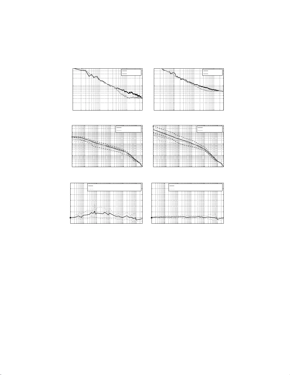
Original Paper
Loading high-quality paper...
Comments & Academic Discussion
Loading comments...
Leave a Comment