In this series of seven papers, predominantly by means of elementary analysis, we establish a number of identities related to the Riemann zeta function. Whilst this paper is mainly expository, some of the formulae reported in it are believed to be new, and the paper may also be of interest specifically due to the fact that most of the various identities have been derived by elementary methods.
Deep Dive into Some series and integrals involving the Riemann zeta function, binomial coefficients and the harmonic numbers. Volume II(a).
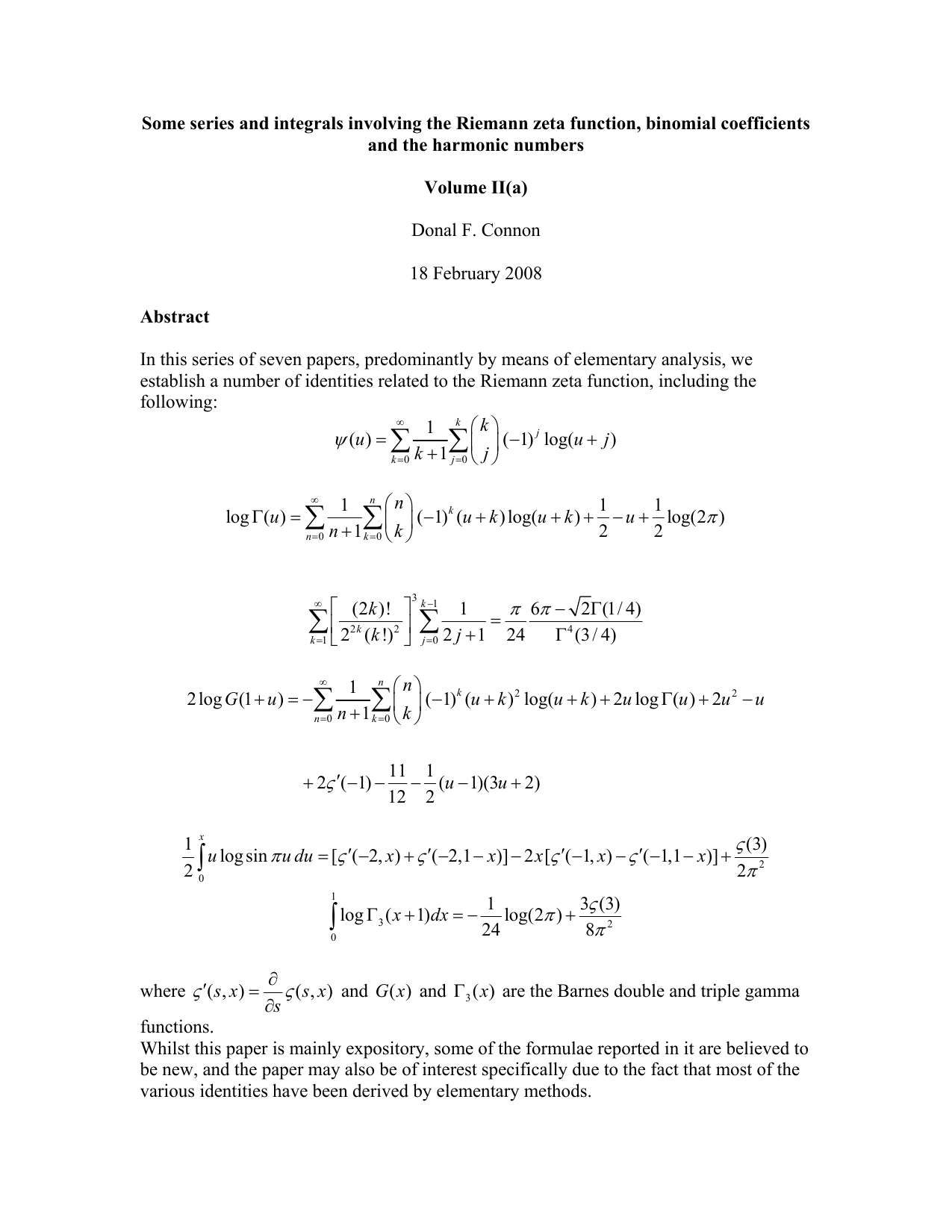
In this series of seven papers, predominantly by means of elementary analysis, we establish a number of identities related to the Riemann zeta function. Whilst this paper is mainly expository, some of the formulae reported in it are believed to be new, and the paper may also be of interest specifically due to the fact that most of the various identities have been derived by elementary methods.
( 1) log( ) 1
0 0 1 2 log (1 ) ( 1) ( ) log( ) 2 log ( ) 2 1 11 1 2 ( 1) ( 1)(3 2) 12 2 1) log( 2 Whilst this paper is mainly expository, some of the formulae reported in it are believed to be new, and the paper may also be of interest specifically due to the fact that most of the various identities have been derived by elementary methods. In this part we derive alternative proofs of the Flajolet and Sedgewick identities (3.16a), (3.16b) and (3.16c) contained in Volume I.
First of all, we consider the following integral (using L’Hôpital’s rule we note that the integrand remains finite as 0 x → ) (4.1.1) 0 1 (1 )
Using the binomial expansion we have (4.1.2) 0 (1 ) ( 1)
and J therefore becomes (4.1.3)
Alternatively, using the substitution x u -= 1 in (4.1.1), we get (4.1.4)
(having used the geometric series in the second part).
(4.1.5) 1Equating (4.1.3) and (4.1.5), we obtain This therefore proves the Flajolet and Sedgewick identity (3.16a): see also the collection of formulae at (4.4.155a) et seq.
We previously used the identity (4.1.7) in (3.5), where it was mentioned that the formula was due to Euler. An alternative proof of (4.1.7) was given by Buschman [37] Formula (4.1.7b) is contained in Higher Transcendental Functions by Erdélyi et al. [58b] and is convergent for Re( ) x a + > 0.
The digamma function is employed later in (4.3.32). Reference should also be made to Appendix E of Volume VI for more details of the digamma function.
We now divide (4.1.6) by t and integrate over the interval [0, x ] to obtain 1, using (4.1.3).
(4.1.10)
, using (4.1.6).
we obtain (4.1.11) 1, using (4.1.9).
(4.1.12)
, using (4.1.10).
Using (4.1.12) we can write (4.1.13)
From the formula (3.17) given by Adamchik we have (4.1.14)
and hence we have an alternative derivation of Flajolet and Sedgewick’s formula (3.16b). (4.1.15) ( )
As a matter of interest, I also found formula (4.1.14) reported by M.E. Levenson in a 1938 volume of The American Mathematical Monthly [98] in a problem concerning the evaluation of (4.1.15a) . A different proof of (4.1.15a) is given in Appendix E of Volume VI.
We can repeat the exercise again by dividing (4.1.10) by x and integrating over the interval [0, t ]. This results in (4.1.16) Quite obviously the method may be extended to produce identities for
where s is an integer.
The formula (4.1.18) is not new: the following generalised identity is referred to as Dilcher’s formula in the Mathworld website [134] and also see the papers by Dilcher [54], Hernández [79] and Prodinger [109]. (4.1.18a)
Reference should also be made to (E.60) in Volume VI for the following identity given by Olds [94aa] in 1936 (4.1.18b)
Dividing (4.1.9) by x , and integrating as before, we obtain (4.1.19) 1and, using (4.1.13) to substitute for the sum in parentheses, we get (4.1.20)
The formula (4.1.21) was obtained by substituting the equivalent of (4.1.14) in (4.1.20). Formula (4.1.21) is the same as Adamchik’s result (3.20c) and hence we have an alternative proof of the Flajolet and Sedgewick equation (3.16c) for ) 3 ( n S (which is rather good news because the author has still not familiarised himself with Mellin transforms, Rice/Nörlund integrals and Bell polynomials!).
We therefore have the following useful identities: (4.1.22a)
We also note that Spieß [123bi] has derived the following identities (4.1.22d) (1)
Note that the coefficients in the final identity are the same as (4.3.26).
Some additional identities involving the harmonic numbers are considered below.
Let us revisit equation (4.1.6) 1 1
( 1) 1and if we let 1 t t → -, we have (1 ) 1 ( 1)
and this can be written as (1 ) 1 ( 1)
Dividing by t we get
Dividing by t and integrating in the range [1, ] t we obtain Four other very different proofs of (4.1.25) are contained in [17a] (and (4.1.24) corrects the minor misprint contained in the solution provided by O.P. Lossers).
In one of the solutions to (4.1.25) in [17a], A.N.’t Woord employs the relation (4.1.26) 1
which is easily proved by mathematical induction. It is clear that (4.1.26) is true for 1 n = and for n > 1 we have
Applying this identity to (3.16a) we have (as was obtained previously in (4.1.12)). Repeating the process we may easily derive the identity in (4.1.18)
Using (4.1.23b) and (4.1.26) we see that (4.1.27) (2)
(1) 1 2 1 1
( 1)
We now refer back to (4.1.25) ( 3 ) 1 0
1 1 (1 ) ( 1) log
1 0 1 (1 ) 1 ( 1) log
and, using (4.1.6), this may be written as
This then gives us (4.1.28) [ ]
log (1 )[ ( ) (3)] 2 We know from [75, p.188
(An alternative proof of (4.2.1) is contained in (4.4.1). I subsequently discovered that yet another proof, using partial fractions, is contained in Further Mathematics [108, p.43]: I must have read, and since forgotten, that proof when I was 17!). The connection between ( ) g x and the gamma function ( ) x Γ is referred to in more detail in Appendix E of Volume VI.
In passing, we note that an application of (4.1.26) to (4.2.1) resul
…(Full text truncated)…
This content is AI-processed based on ArXiv data.