Verified Real Number Calculations: A Library for Interval Arithmetic

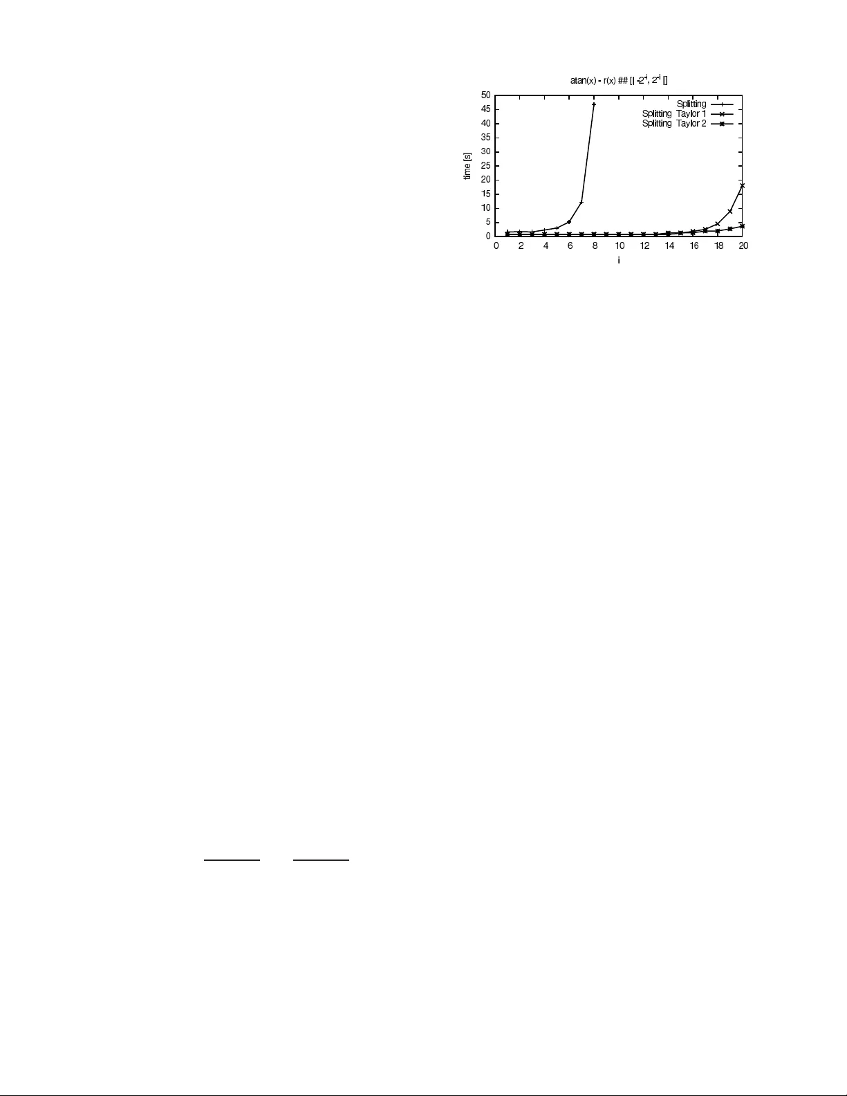
1 V erified Real Number Calc ulations: A Library for Interv al Arithmetic Marc Daumas, David Lester , and César Muñoz Abstract — Real number calculations on elementary fun ctions are remar kably diffi cult to handl e in mechanical proofs. In this paper , we show how these calculations can b e performed within a theorem prov er or proof assistant in a con ve nient and h ighly automated as well as interacti ve way . First, we f orma lly establish upper and lower bound s for el ementary fu nctions. Then, based on these bound s, we dev elop a rational interv al arithmetic where real number calculations take place in an algebraic settin g. In order to reduce the dependency effect of interv al arithmetic, we integrate two techniq ues: int erv al sp litting and taylor series expansions. This pragmatic approach has been developed, and fo rmally verified, in a theorem prov er . The forma l d ev elopment also incl udes a set of customizable strategies to automate proofs in volving expl icit calculations ov er real numbers. Our ul timate goal is to p ro vide guara nteed pro ofs of numerical pro perties with minimal human theorem-prov er interaction. Index T erms — Real number calculations, interva l arithmetic, proof checki ng, theorem proving I . I N T RO D U C T I O N Deadly and disastro us failures [1]–[ 3] confirm the shar ed belief that trad itional testing, simulation , and peer-revie w are not suf ficient to guarantee the correctness of critical soft- ware. F ormal Methods in compu ter science refer s to a set of mathem atical techniqu es and too ls to verif y saf ety p rop- erties of a system design an d its impleme ntation fu nctional requirem ents. In th e verification of eng ineering applicatio ns, such as aer ospace systems, it is o ften nece ssary to p erform explicit calculations with n on-alge braic functions. Despite all of the developments concerning real analysis in theorem provers [4]–[8 ], the formal verification of the corr ectness of these calculations is no t routin e. T ake, for example, the for mula 3 π 180 ≤ g v tan( 35 π 180 ) ≤ 3 . 1 π 180 , (1) where g is the gr avitational force and v = 250 knots is the groun d sp eed of an aircra ft. This formu la app ears in the verification of N ASA ’ s Airborn e Info rmation fo r Lateral Spacing (AILS) algo rithm [9]. It states that the turn rate of an aircra ft flying at g round speed v with a bank angle of 35 o is about 3 o per second. A direct proof of this f ormula is M. D aumas ( marc.dauma s@lirmm.fr ) is with the LIRMM, CNRS, UM2 and EL IA US, UPVD and he is supported in part by the PICS 2533 of the CNRS. D. Lester ( dlester@cs. man.ac.uk ) is with the Uni ve rsity of Manch- ester , Oxford Road, Manchester M13 9PL, UK and he is supported in part by the French Région Languedoc- Roussillon . C. Muñoz ( munoz @nianet.org ) is with the Nationa l Institute of Aerospace , 100 Exploration W ay , Hampton, V A 23666, USA and he is supported in part by he Natio nal Aeronautics and Space Administrati on under NASA Cooperat i ve Agreement NCC-1-02043 and by the Uni v ersity of Perpignan. about a pag e long and requir es the use of several trigonometric proper ties. In many cases the formal checking of numerica l calculations is so cumbersome that the ef fort seems futile; it is then tempting to perf orm th e calculation s ou t of the system, and introdu ce th e resu lts as axioms. 1 Howe ver , chances ar e that the external calculations will be performed using floating-point arithmetic. Wi thout formal checkin g o f the results, we will never be sur e o f the correctn ess of th e c alculations. In this paper we p resent a set of interactive tools to auto mat- ically prove num erical p roperties, such as Formula (1), within a proof assistant. The point of departure is a collection of lower and upper b ounds for rational and non-ration al o perations. Based on provable prop erties of these bo unds, we develop a rational interval a rithmetic wh ich is amen able to automation. The series approximatio ns and interval arithm etic presented here ar e well-k nown. Howe ver , to o ur kn owledge, th is is the most com plete formaliza tion in a theorem p rover of interval arithmetic that includ es non -algebraic f unctions. Our ultimate g oal is to provide guaranteed f ormal p roofs of num erical prop erties with minimu m hum an effort. As automated proce sses are bo und to fail on degen erate cases and waste time and me mory on simple ones, we hav e d esigned a set of h ighly cu stomizable p roof strategies. T he d efault values of the parameters are sufficient in most simple cases. Howe ver , a d omain expert can set these p arameters to obtain a desired result, e.g. , the accura cy of a particular calculation. This pa per merges an d extend s the resu lts presented in [10], [1 1]. The rest of th is do cument is organized as follows. Section II defines bo unds fo r elem entary f unctions. Sec tion I II presents a rational interval arith metic based o n th ese b ounds. Section IV describ es a m ethod to prove numeric al propo si- tions. The imp lementation of this m ethod in a theore m pr over is described in Sectio n V. L ast section summar izes ou r work and co mpares it to related work. The mathema tical development presented in this pa per ha s been written and fully verified in th e Pro totype V erification System ( PVS) [12] 2 . PVS provides a strongly typed specifica- tion language and a theorem prover for higher-order logic. It is developed by SRI In ternational. Our dev elopment is freely av ailable on the Inte rnet. The results o n upper and lower boun ds have been integrated to the NASA Langley PVS Libraries 3 and the rational interval arithmetic and the PVS strategies fo r num erical p roposition s are available fr om on e of 1 As a matter of fact , the original verificati on of NASA ’ s AILS algorithm contai ned se vera l such axioms. 2 PVS is av ailabl e from http: //pvs.csl.sri.c om . 3 http://shemesh .larc.nasa.gov/f m/ftp/larc/PVS- library/pvslib.h t m l the authors 4 . For readability , we will use standard m athematical no tations along th is p aper and PVS n otations will be limited to illustrate the use of the libr ary . In the following, we use the first letters of the alphabet a, b , . . . to denote rationa l nu mbers, and the last letters o f the alpha bet . . . x, y , z to denote arbitrary re al variables. W e use bo ldface for inter val variables. Furthermor e, if x is an interval variable, x denotes its lower b ound an d x denotes its up per boun d. I I . B O U N D S F O R E L E M E N TA RY F U N C T I O N S A PVS basic the ory of bou nds for square root and trigono - metric fu nctions was originally pro posed for th e verification of N ASA ’ s A ILS a lgorithm [9 ]. W e have co mpleted it and extended with b ound s fo r natural logarithm , expone ntial, and arctangen t. Th e basic idea is to provide for eac h real f unction f : R 7→ R , func tions f : ( R , N ) 7→ R and f : ( R , N ) 7→ R closed un der Q , such that f or all x , n f ( x, n ) ≤ f ( x ) ≤ f ( x, n ) , (2) f ( x, n ) ≤ f ( x, n + 1) , (3) f ( x, n + 1) ≤ f ( x, n ) , (4) lim n →∞ f ( x, n ) = f ( x ) = lim n →∞ f ( x, n ) . (5) Formula (2) states that f and f are, resp ectiv ely , lower and upper boun ds of f , and formu las (3), (4), and (5) state that these bo unds can ultimately b e imp roved, as mu ch as need ed, by in creasing the app roximation parameter n . For transcendental functio ns, we use taylor appr oximation series. W e pe rformed a co arse range red uction [13] since the conv ergence of taylor series is usually best for small values. More elaborate range redu ction techniq ues [1 4] would signif- icantly en hance the speed and the accura cy of the func tions defined in Sections II and III. All the stated propositions in this section have b een fo rmally verified in th e verification system PVS. A. Squ ar e r oot For s quare root, we use a simple approx imation by Newton’ s method. For x ≥ 0 , sqrt( x, 0) = x + 1 , sqrt( x, n + 1) = 1 2 ( y + x y ) , where y = sqrt( x, n ) , sqrt( x, n ) = x sqrt( x, n ) . Pr oposition 1 : ∀ x ≥ 0 , n : 0 ≤ sqrt ( x, n ) ≤ √ x < sqrt( x, n ) . The first inequ ality is strict when x > 0 . 4 http://researc h.nianet.org/~mu noz/Interval . B. T rig onometric fu nctions W e u se the p artial app roximation by serie s. sin ( x, n ) = m X i =1 ( − 1) i − 1 x 2 i − 1 (2 i − 1)! sin( x, n ) = m +1 X i =1 ( − 1) i − 1 x 2 i − 1 (2 i − 1)! , cos ( x, n ) = 1 + m +1 X i =1 ( − 1) i x 2 i (2 i )! , cos( x, n ) = 1 + m X i =1 ( − 1) i x 2 i (2 i )! , where m = 2 n if x < 0 ; oth erwise, m = 2 n + 1 . Pr oposition 2 : ∀ x, n : sin ( x, n ) ≤ sin( x ) ≤ sin( x , n ) . Pr oposition 3 : ∀ x, n : cos ( x, n ) ≤ cos( x ) ≤ cos( x, n ) . C. Ar ctangent an d π W e first use the alternating p artial appro ximation by series for 0 ≤ x ≤ 1 . atan( x, n ) = 2 n +1 X i =1 x 2 i +1 ( − 1) i 2 i + 1 , if 0 < x ≤ 1 , atan( x, n ) = 2 n X i =1 x 2 i +1 ( − 1) i 2 i + 1 , if 0 < x ≤ 1 . W e no te that for x = 1 (which we migh t naïvely wish to use to define π / 4 and hence π ) th e series: 1 − 1 3 + 1 5 − 1 7 + 1 9 − · · · does conv erge, but very slo wly . Instead, we u se the equality π 4 = 4 atan(1 / 5) − atan(1 / 23 9) , tha t h as mu ch b etter co n vergence proper ties. Using this identity we can d efine bo unds on π : π ( n ) = 16 a tan(1 , n ) − 4 atan(1 , n ) , π ( n ) = 16 atan(1 , n ) − 4 a ta n(1 , n ) . Pr oposition 4 : ∀ n : π ( n ) ≤ π ≤ π ( n ) . Now , using prop erties o f arctangen t, we extend the range of the fu nction to the whole set of r eal num bers: atan(0 , n ) = atan(0 , n ) = 0 , atan ( x, n ) = π ( n ) 2 − atan( 1 x , n ) , if 1 < x, atan ( x, n ) = − atan( − x, n ) , if x < 0 , atan( x, n ) = π ( n ) 2 − atan ( 1 x , n ) , if 1 < x, atan( x, n ) = − atan( − x, n ) , if x < 0 . Pr oposition 5 : ∀ x, n : atan ( x, n ) ≤ atan( x ) ≤ atan( x, n ) . These are strict ineq ualities except when x = 0 . The PVS definition o f bo unds on atan and π are presen ted in L isting 1. PVS developments are organized in theories, which are collections of mathematical and logical objects such a s f unction definitio ns, variable decla rations, axioms, and lemmas. The a tan_approx th eory first imports th e definition of the arctange nt function. Then, it declares v ariables n,x,px of types nat ( natural n umbers) , real (real nu m- bers), and posrea l (p ositiv e real number s), respectively . For the scope of the theory , th ese variables are imp licitly univer - sally quantified . Though writing definitio ns, lemmas, theor ems and specially p roofs in PVS requires some training, reading theories is p ossible to anyb ody with a m inimal backg round in logic. D. Expo nential The series we use for the expo nential function is exp( x ) = ∞ X i =0 x i i ! . W e co uld directly fin d bou nds f or negative x fr om this series as, in this case, the series is alternating. Howe ver , we will subsequen tly find that it is co n venient to show that our bou nds for the exponential function are strictly po siti ve, and this is no t true fo r all x ≤ 0 . Y et, this pro perty holds fo r − 1 ≤ x ≤ 0 . W e define exp ( x, n ) = 2( n +1)+1 X i =0 x i i ! , if − 1 ≤ x < 0 , exp( x, n ) = 2( n +1) X i =0 x i i ! , if − 1 ≤ x < 0 . Using p roperties o f the exponential functio n, we obtain bound s f or the whole set of real nu mbers: exp (0 , n ) = exp(0 , n ) = 1 , exp ( x, n ) = exp( x −⌊ x ⌋ , n ) −⌊ x ⌋ , if x < − 1 exp ( x, n ) = 1 exp( − x, n ) , if x > 0 , exp( x, n ) = exp( x −⌊ x ⌋ , n ) −⌊ x ⌋ , if x < − 1 exp( x, n ) = 1 exp( − x, n ) , if x > 0 . Notice that unless we can ensure that all of the bounding function s are strictly positiv e we will run into type-check ing problem s using the bound de finitions for x > 0 , e.g. , 1 / exp( − x, n ) is o nly defined provided exp( − x, n ) 6 = 0 . Pr oposition 6 : ∀ x, n : 0 < exp ( x, n ) ≤ exp( x ) ≤ exp( x, n ) . These are strict ineq ualities except when x = 0 . E. Natural Logarithm For 0 < x ≤ 1 , we use the alternating series for natural logarithm : ln( x + 1) = ∞ X i =1 ( − 1) i +1 x i i . PVS Listing 1 Definition of b ounds on atan and π atan_approx: THEORY BEGIN IMPORTING atan n: VAR nat x: VAR real px: VAR posreal atan_pos_le1_u b(n,x): real = atan_series_n( x,2 * n) atan_pos_le1_l b(n,x): real = atan_series_n( x,2 * n+1) atan_pos_le1_b ounds: LEMMA 0 < x AND x <= 1 IMPLIES atan_pos_le1_l b(n,x) < atan(x) AND atan(x) < atan_pos_le1_ub(n, x) pi_lbn(n): posreal = 4 * (4 * atan_pos_le1_l b(n,1/5) - atan_pos_le1_u b(n,1/239)) pi_ubn(n): posreal = 4 * (4 * atan_pos_le1_u b(n,1/5) - atan_pos_le1_l b(n,1/239)) pi_bounds: THEOREM pi_lbn(n) < pi AND pi < pi_ubn(n) atan_pos_lb(n, px): real = IF px <= 1 THEN atan_pos_le1_l b(n,px) ELSE pi_lbn(n)/2 - atan_pos_le1_u b(n,1/px) ENDIF atan_pos_ub(n, px): real = IF px <= 1 THEN atan_pos_le1_u b(n,px) ELSE pi_ubn(n)/2 - atan_pos_le1_l b(n,1/px) ENDIF atan_lb(x,n): real = IF x > 0 THEN atan_pos_lb(n, x) ELSIF x = 0 THEN 0 ELSE -atan_pos_ub(n,- x) ENDIF atan_ub(x,n): real = IF x > 0 THEN atan_pos_ub(n, x) ELSIF x = 0 THEN 0 ELSE -atan_pos_lb(n,- x) ENDIF atan_bounds: THEOREM atan_lb(x,n) <= atan(x) AND atan(x) <= atan_ub(x, n) END atan_approx Therefo re, we defin e ln ( x, n ) = 2 n X i =1 ( − 1) i +1 ( x − 1) i i , if 1 < x ≤ 2 , ln( x, n ) = 2 n +1 X i =1 ( − 1) i +1 ( x − 1) i i , if 1 < x ≤ 2 . Using pr operties of the natural logarith m fun ction, we obtain ln (1 , n ) = ln(1 , n ) = 0 ln( x, n ) = − ln( 1 x , n ) , if 0 < x < 1 , ln( x, n ) = − ln( 1 x , n ) , if 0 < x < 1 . Finally , we extend the rang e to the wh ole set o f positive r eals. If x > 2 , we find a n atural nu mber m an d real numb er y such that x = 2 m y and 1 < y ≤ 2 , b y u sing th e following recu rsi ve algorithm similar in spirit to Euclide an division: lnnat(x:posre al,k:posnat): [nat ,posreal] = if x < k then (0,x) else let (m,y) = lnnat(x/k,k) in (m+1,y) endif W e next p rove the fo llowing prop erty: Pr oposition 7 : ∀ x ≥ 1 , k > 1 : k m ≤ x < k m +1 , y < k , x = k m y , wh ere ( m, y ) = l nnat ( x, k ) . If ( m, y ) = ln nat (2 , x ) , we o bserve that ln( x ) = ln(2 m y ) = m ln(2 ) + ln( y ) . Hence, ln ( x, n ) = m ln(2 , n ) + ln( y , n ) , if x > 2 , ln( x, n ) = m ln(2 , n ) + ln( y , n ) , if x > 2 . Pr oposition 8 : ∀ x > 0 , n : ln ( x, n ) ≤ ln( x ) ≤ ln( x, n ) . These are strict ineq ualities except when x = 1 . I I I . R AT I O NA L I N T E R V A L A RI T H M E T I C Interval arithme tic has b een u sed for decad es as a standard tool for nu merical analysis on en gineering application s [15 ], [16]. In interval arith metic, o perations are evaluated on r ange of nu mbers rather than o n real numbe rs. A (closed) interva l [ a, b ] is the set o f real nu mbers between a an d b , i.e. , [ a, b ] = { x | a ≤ x ≤ b } . The bou nds a and b ar e called th e lower bou nd and up per bound of [ a, b ] , respectively . Note that if a > b , the interval is the em pty set. The notation [ a ] ab breviates the po int-wise interval [ a, a ] . Interval compu tations can be perform ed on the en dpoints or on the center and th e radiu s. For this work , we d ecided to work on r ational e ndpoin ts. Trigonometric and transcen dental function s fo r inter val arithmetic are d efined using the bo unds presented in Section II. Listing 2 shows a few definitions fro m the PVS the- ory Interv al . Do ts are used to simp lify the presenta tion and h ide some technical p arts. The theory defines the typ e Interval as a record with fields ub and l b of typ e rat (rational numbe rs), variables x,y of type real , variable n of typ e nat , and variables X,Y of ty pe Inter val . PVS Listing 2 Definition of in terval arithm etic Interval : THEORY BEGIN Interval : TYPE = [# lb : rat, ub : rat #] x,y : VAR real n : VAR nat X,Y : VAR Interval +(X,Y): Interval = [|lb(X)+lb(Y ), ub(X)+ub(Y)|] -(X,Y): Interval = [|lb(X)-ub(Y ), ub(X)-lb(Y)|] -(X) : Interval = [|-ub(X), -lb(X))|] * (X,Y): Interval = ... /(X,Y): Interval = X * [|1/ub(Y), 1/lb(Y)|] Abs(X): Interval = ... Sq(X) : Interval = ... ^(X,n): Interval = ... U(X,Y) : Interval = [|min(lb(X) ,lb(Y)), max(ub(X),ub( Y))|] ... END Interval If X is a PVS interval, lb(X) is the lower bo und and ub(X) is the upper b ound of X . In PVS, we define the syntactic sugar [| x,y|] to represent th e interval [ x, y ] . Interval union x ∪ y , written in PVS X U Y , is defined as the smallest rationa l interval that co ntains bo th x and y . The four basic interval o peration s are defin ed as fol- lows [17]: x + y = [ x + y , x + y ] , x − y = [ x − y , x − y ] , x × y = [min { xy , x y , x y , x y } , max { xy , xy , xy , xy } ] , x / y = x × [ 1 y , 1 y ] , if yy > 0 . W e also d efine the unary negation , absolute value, an d power operator s f or inter vals: − x = [ − x , − x ] , | x | = [min {| x | , | x |} , max {| x | , | x |} ] , if x x ≥ 0 . | x | = [0 , max {| x | , | x |} ] , if xx < 0 . x n =        [1] if n = 0 , [ x n , x n ] if x ≥ 0 or od d? ( n ) , [ x n , x n ] if x ≤ 0 and even? ( n ) , [0 , max { x n , x n } ] otherwise . Interval operatio ns are defined such that they inclu de th e result of their correspo nding real opera tions. This prop erty is called the inc lusion pr operty . Pr oposition 9 (Inclusion Pr operty for Basic Operators): If x ∈ x an d y ∈ y then x ⊗ y ∈ x ⊗ y , where ⊗ ∈ { + , − , × , / } . Moreover , − x ∈ − x , | x | ∈ | x | , and x n ∈ x n , for n ≥ 0 . It is assumed that y does not contain 0 in th e case o f interval division. Listing 3 specifies this property in PVS. The propo sition x ∈ x is written x ## X . PVS Listing 3 Basic inc lusion p roperties Add_inclusion : LEMMA x ## X AND y ## Y = ⇒ x+y ## X+Y Sub_inclusion : LEMMA x ## X AND y ## Y = ⇒ x-y ## X-Y Neg_inclusion : LEMMA x ## X = ⇒ -x ## -X Mult_inclusio n : LE MMA x ## X AND y ## Y = ⇒ x * y ## X * Y Div_inclusion : LEMMA NOT 0 ## Y AND x ## X AND y ## Y = ⇒ x/y ## X/Y Abs_inclusion : LEMMA x ## X = ⇒ abs( x) ## abs(X) Sq_inclusion : LEMMA x ## X = ⇒ sq(x ) ## sq(X) Pow_inclusion : LEMMA x ## X = ⇒ x^n ## X^n The inclu sion property is fund amental to interval arithmetic. It guarante es that evaluations of an expr ession using interval arithmetic bo und its exact real value. Any oper ation in in terval arithmetic must satisfy the inclu sion proper ty with respec t to its correspo nding r eal oper ation. A. Interva l compa risons There a re several possible ways to c ompare intervals [18]. In this work, we use interval-rational comp arisons and interval inclusions. x < a if x < a, similarly fo r ≤ , x > a if x > a, similarly for ≥ , x ⊆ y if y ≤ x an d x ≤ y . Pr oposition 1 0: Assume that x ∈ x , 1) if x ⊲ ⊳ a th en x ⊲ ⊳ a , for ⊲ ⊳ ∈ { <, ≤ , > , ≥} , and 2) if x ⊆ y then x ∈ y . W e use 6 ⊲ ⊳ to deno te ≥ , > , ≤ , or < , when ⊲ ⊳ is, respec ti vely , < , ≤ , > , or ≥ . Pr oposition 1 1: If x ⊲ ⊳ a and x 6 ⊲ ⊳ a , then x is empty . Notice that ¬ ( x ⊲ ⊳ a ) does not imp ly x 6 ⊲ ⊳ a . For instance, [ − 1 , 1 ] is n either g reater nor less than 0 . B. Squ ar e r oot, ar ctangent, e xponentia l, an d natural loga- rithm Interval fu nctions for square root, ar ctangent, π , expon en- tial, an d n atural log arithm are defined for an approx imation parameter n ≥ 0 : [ √ x ] n = [sqrt( x , n ) , sqrt( x , n )] , if x ≥ 0 , [atan( x )] n = [atan( x , n ) , a tan( x , n )] , [ π ] n = [ π ( n ) , π ( n )] , [exp( x )] n = [exp ( x , n ) , exp( x , n )] , [ln( x )] n = [ln ( x , n ) , ln( x , n )] , if x > 0 . As c onsequen ce of Propo sitions 1, 5, 6, an d 8 in Sec tion I I, and the fact that these f unctions ar e inc reasing, the above function s satisfy the following inclusion prop erty . Pr oposition 1 2: For all n , if x ∈ x th en f ( x ) ∈ [ f ( x )] n , where f ∈ { √ , atan , exp , ln } . Moreover , π ∈ [ π ] n . It is assumed that x is non-n egati ve in the ca se of squ are ro ot, and x is positive in the case o f natural log arithm. C. T rigon ometric functions Parametric functions for interval trigonometric function s are defined by cases an alysis on quadr ants wh ere the func tions are in creasing or decreasing . The mathematica l definitio ns are presented in Figu re 1. Note that sin and cos are defined f or the whole real line. Howe ver , fo r an gles α such th at | α | > π both f unctions will return the inter val [ − 1 , 1] , a valid b ound but no t a very g ood one. Furthermor e, the expression n + 5 in Formula (8) is necessary to gu arantee that lower an d up per bound s of co sine are strictly positi ve in the interval [ − π ( n +5) 2 , π ( n +5) 2 ] , and thus, the interval tangent func tion is always defined in that inter val. The interval trig onometr ic func tions satisfy th e inclusion proper ty . Pr oposition 1 3: If x ∈ x th en f ( x ) ∈ [ f ( x )] n , wh ere f ∈ { sin , cos } . Mo reover , if x ⊆ [ − π ( n +5) 2 , π ( n +5) 2 ] , tan( x ) ∈ [tan( x )] n . The next sectio n p roposes a method to prove numerical propo sitions based on the interval arithmetic de scribed h ere. I V . M E C H A N I C A L P R O O F S O F N U M E R I C A L P RO P O S I T I O N S Arithmetic expr ession s are d efined by the following gr am- mar , where V is an denum erable set of real variables: e ::= a | x | e + e | e − e | − e | e × e | e/e | | e | | e i | √ e | π | sin( e ) | cos( e ) | tan( e ) | exp( e ) | ln( e ) | a tan( e ) a ∈ Q i ∈ N x ∈ V Numerical pro positions P have either the fo rm e 1 ⊲ ⊳ e 2 , where ⊲ ⊳ ∈ { <, ≤ , >, ≥} , o r th e form e ∈ a , whe re a is a constant inter val (an interval with con stant ratio nal endp oints). As usual, parentheses are used to group real and interval expressions as n eeded. [sin( x )] n =            [sin ( x , n ) , sin( x , n )] if x ⊆ [ − π ( n ) 2 , π ( n ) 2 ] , [sin ( x , n ) , sin( x , n )] else if x ⊆ [ π ( n ) 2 , π ( n )] , [min { sin( x , n ) , sin( x , n ) } , 1 ] else if x ⊆ [0 , π ( n )] , − [sin( − x )] n else if x ⊆ [ − π ( n ) , 0] , [ − 1 , 1 ] otherwise , (6) [cos( x )] n =        [cos ( x , n ) , cos( x , n )] if x ⊆ [0 , π ( n )] , [cos( − x )] n else if x ⊆ [ − π ( n ) , 0] , [min { cos ( x , n ) , cos( x , n ) } , 1] else if x ⊆ [ − π ( n ) 2 , π ( n ) 2 ] , [ − 1 , 1 ] otherwise , (7) [tan( x )] n = [ sin cos ( x , n + 5) , sin cos ( x , n + 5 )] , if x ⊆ [ − π ( n + 5) 2 , π ( n + 5) 2 ] . (8) Fig. 1. Interv al trigonometric functi ons A context Γ is a set of hypoth eses of the form x ∈ x . A gr ound context is a context where all the intervals ar e constant. In the following, we u se logical judgments in the sequent calculu s style, e.g. , Γ ⊢ P , wh ere all free variables occurrin g in P ar e in Γ . T he intend ed semantics of a judgme nt Γ ⊢ P is that the numer ical pro position P is true under th e hypoth eses Γ . Giv en a context Γ , an appr oximation p arameter n , and an expression e , such that the free variables of e are in Γ , we define th e interval expression [ e ] Γ n by re cursion on e . [ a ] Γ n = [ a ] , [ x ] Γ n = x , where ( x ∈ x ) ∈ Γ , [ e 1 ⊗ e 2 ] Γ n = [ e 1 ] Γ n ⊗ [ e 2 ] Γ n , where ⊗ ∈ { + , − , × , / } , [ e i ] Γ n = ([ e ] Γ n ) i , [ − e ] Γ n = − [ e ] Γ n , [ | e | ] Γ n = | [ e ] Γ n | , [ π ] Γ n = [ π ] n , [ f ( x )] Γ n = [ f ([ x ] Γ n )] n , where f ∈ { sin , cos , tan , exp , ln , a tan } . Theor em 1 (In clusion): Let Γ be a context, n an appro xi- mation para meter , and e a well-defined arithmetic expression in Γ , i.e. , side co nditions for d ivision, squar e root, log arithm, and tan gent are satisfied, Γ ⊢ e ∈ [ e ] Γ n . (9) Pr oof: By structu ral induction on e and proposi- tions 4, 9, 12, and 13. A. A general method for n umerical p r o positions W e p ropose a g eneral metho d to prove numerica l pr oposi- tions. First, con sider a judg ment o f the fo rm Γ ⊢ e 1 ⊲ ⊳ e 2 , where Γ is a grou nd c ontext. 1) Select an a pprox imation parameter n . 2) Define e = e 1 − e 2 . 3) Ev aluate [ e ] Γ n ⊲ ⊳ 0 . If it ev aluates to true, th e following judgmen t h olds Γ ⊢ [ e ] Γ n ⊲ ⊳ 0 . In tha t case go to step 5 . 4) Ev aluate [ e ] Γ n 6 ⊲ ⊳ 0 . If th is ev aluates to tr ue then fail. By Proposition 11, the judgment Γ ⊢ [ e ] Γ n ⊲ ⊳ 0 cann ot hold. If [ e ] Γ n 6 ⊲ ⊳ 0 ev aluates to false, increase the approximation parameter an d retu rn to step 3. 5) By Theo rem 1 , Γ ⊢ e ∈ [ e ] Γ n . 6) Proposition 10 yields Γ ⊢ e ⊲ ⊳ 0 . 7) By definition , Γ ⊢ e 1 − e 2 ⊲ ⊳ 0 . 8) Therefore, Γ ⊢ e 1 ⊲ ⊳ e 2 . The me thod ab ove c an be easily ad apted to judg ments of the for m Γ ⊢ e ⊲ ⊳ a . In this c ase, the inter val expression [ e ] Γ n ⊆ a is evaluated. If the expression evaluates to true, then the o riginal judgm ent hold s by The orem 1 and Pro position 1 0. Otherwise, th e metho d should fail. The gen eral method is sou nd , i.e. , all the steps can be effecti vely computed and each one is formally justified. In particular, the pro positions [ e ] Γ n ⊲ ⊳ 0 , [ e ] Γ n 6 ⊲ ⊳ 0 , and [ e ] Γ n ⊆ a can be mec hanically com puted as they only in volv e rational arithmetic a nd constant numerical values. The method is not complete as it d oes not necessarily term inate. Even if e only in volves the four basic operation s and n o variables, it may be that bo th [ e ] Γ n ⊲ ⊳ 0 and [ e ] Γ n 6 ⊲ ⊳ 0 evaluate to false. The absence o f a co mpleteness result is a fundamen tal limitation on any gene ral computable arithmetic. At a practica l lev el, the problem arises because all we h av e av ailable ar e a sequenc e o f appro ximations to the real numb ers x and y ; provided x an d y differ , with luck we will eventually have a p air of appro ximations who se in tervals do n ot overlap, and hence we can return a result for x ⊲ ⊳ y . H owe ver , if x and y are the same real numb er (n ote we migh t no t n ecessarily get the same sequ ence of approx imations f or both x and y ), we can never b e sure w hether fur ther e valuation mig ht result in us b eing able to distinguish the nu mbers. B. Depen dency effect The d ependen cy effect is a well-known b ehavior of in terval arithmetic due to the f act that interval identity is lost in interval ev aluations. This may have surprising results, fo r instance x − x is [0] only if x is poin t-wise. Moreover , as we have seen in Section III-A, both x ≥ a and x < a may be false. Add itionally , interval arith metic is subdistributi ve, i.e. , x × ( y + z ) ⊆ x × y + x × z . In th e general case the inclu sion is strict and some dep endency effects appear as soon as a variable is u sed mor e than once in an expr ession. For the metho d presented in Section IV -A, it means that the arrange ment o f th e expre ssion e ma tters. For instan ce, assum e that we want to p rove x ∈ [0 , 1] ⊢ 2 × x ≥ x . This is pretty obvious in ar ithmetic as x is a non-negative re al. Using o ur me thod, we first consider the arithme tic expression e = 2 × x − x and then construct the interval expression [ e ] Γ n = 2 × x − x , where x = [0 , 1] . For any ap proxim ation parameter n , [ e ] Γ n ev aluates to [ − 1 , 2] wh ich is n either greater nor less than 0 . The refore, the metho d will not term inate. On the other hand, if instead o f the arithmetic expression 2 × x − x , we consider the eq uiv alent arithmetic expression x , we have [ x ] Γ n = [0 , 1] and [0 , 1] ≥ 0 evaluates to true. A second observation is th at because of the dependen cy effect th e wid th of intervals also m atters. Co nsider ag ain the expression e = 2 × x − x . W e have seen that the interval ev aluation of [ e ] Γ n , for x ∈ [0 , 1] , results in [ − 1 , 2 ] , which is n ot sufficient to prove that [ e ] Γ n ≥ 0 . On the o ther han d, the expression [ e ] Γ n ev aluates to [ − 1 / 2 , 1] when x ∈ [0 , 1 / 2 ] and it e valuates to [0 , 3 / 2 ] wh en x ∈ [1 / 2 , 1 ] . Therefo re, we can prove that, for x ∈ [0 , 1 ] , [ e ] Γ n ⊆ [ − 1 / 2 , 1] ∪ [0 , 3 / 2] , i.e. , [ e ] Γ n ⊆ [ − 1 / 2 , 3 / 2] , which is a better a pprox imation than [ − 1 , 2 ] . I f w e con tinue d ividing the inter val [0 , 1] and com- puting the union of the resulting in tervals, we can eventually prove th at [ e ] Γ n + ǫ ≥ 0 for an a rbitrary small ǫ > 0 . These o bservations lead to two enhan cements of the gener al method. First, we cou ld di vide each inter val in Γ be fore applying the gen eral technique. Second, we may want to replace the origina l expression by an equiv alent one that is less prone to the depe ndency effect. C. In terval splitting In interval arithm etic, th e depen dency effect of the union of the parts is less tha n the depend ency effect o f th e whole. Indeed , the simplest way to r educe the dep endency effect is to divide th e interval variables into se veral tiles (sub intervals) and to e v aluate the original expression on these tiles s eparately . This techniqu e is c alled in terval splitting or sub- paving and is expressed by th e f ollowing d eduction rule. Pr oposition 1 4: Let Γ be a co ntext, e an expression wh ose free variables are x and those in Γ , e an interval expression, and x , x 1 , . . . , x n intervals su ch that x = S 1 ≤ i ≤ n x i , ∀ 1 ≤ i ≤ n : x ∈ x i , Γ ⊢ e ∈ e [Splitting] x ∈ x , Γ ⊢ e ∈ e The Splitting r ule can be iterated to obtain a splitting for multiple variables. No te that the numb er of tiles g enerated b y interval splitting is exponential in the number of variables. Indeed , if k 1 is the numb er o f tiles of th e first variable alone , k 2 is the number of tiles of the second variables alone , and so forth, the total numb er of tiles to be con sidered for m variables is Q 1 ≤ j ≤ m k j . The integration o f the Splitting rule into th e genera l metho d is straig htforward. First, a splitting is co mputed for a given set of variables in Γ . Then, the general method is applied to all cases. If the gen eral method is successfu l in all of th em, by Proposition 14, th e orig inal ju dgment holds. Oth erwise, the method fails and a n ew splitting ma y be considere d. D. T a ylor Series E xpansions Replacing 2 × x − x by x can be do ne au tomatically . In fact, as we will see in Section V, these kind s o f simplificatio ns are perfor med by our PVS imp lementation of the gen eral metho d. Howe ver , th ese simp lifications may n ot be sufficient even for simple expressions suc h as x × (1 − x ) , wh ere x ∈ [0 . 1] . The subdistributi vity p roperty o f interval arithmetic states that the interval ev aluation of x × (1 − x ) is better than that of the equiv alent exp ression x − x 2 . Un fortuna tely , that evaluation is no t goo d en ough to prove that x × (1 − x ) ∈ [0 , 1 / 4] . In this case, as a domain expert k nows, th e optimal an swer is obtained with the equiv alent expr ession 1 / 4 − (1 / 2 − x ) 2 . Th e solution is a lo t less intuitive when non -algebra ic function s are in volved. T aylor’ s theo rem states th at a n -d ifferentiable fu nction c an be app roximated nea r a g iv en p oint b y a polyno mial of d egree n who se co efficients depen d o n th e de riv ati ves of th e fu nction at that point. In interval arith metic, taylor’ s theo rem can be expressed by th e f ollowing dedu ction rule. Pr oposition 1 5: Let x , x 0 , . . . , x n be strictly pro per inter- vals, f a n -differentiable function o n a variable x ∈ x , an d c ∈ x a constant, ∀ 0 ≤ i < n : ⊢ f ( i ) ( c ) ∈ x i x ∈ x ⊢ f ( n ) ( x ) ∈ x n [T aylor] x ∈ x ⊢ f ( x ) ∈ Σ n i =0 ( x i × ( x − c ) i ) /i ! The e xpression of T aylo r’ s rule s hows that interval x appears only once in each term o f o rder i for i b etween 1 and n − 1 preventing any depen dency effect due to x in a term alone. The term of or der n suffers some depend ency effect as x also appears in the defin ition of x n . In mo st cases, n = 2 is used to cancel first order dep endency effects as p resented Listing 4. But in cases whe re th e first der i vati ves nearly vanish or where the e v aluation of the la st deri vati v e introduc es significant depend ency effects, we compute m ore terms to reach some better b ounds. Using T aylor’ s r ule requir e mo re work than the Splitting rule. I n particular , we n eed to provide in tervals x 0 , . . . , x n and constant c that satisfy the hypoth eses of th e rule. For c we choose th e mid dle p oint of x unless the user propo ses an other point. It follow imm ediately that c ∈ x . For 0 ≤ i < n , we choose x i = [ f ( i ) ( c )] n and, by The orem 1, we h av e f ( i ) ( c ) ∈ x i . Finally , we choose x n = [ f ( n ) ( x )] Γ n , where Γ is th e context x ∈ x . By T heorem 1, we have Γ ⊢ f ( n ) ( x ) ∈ x n . In order to prove the judgmen t x ∈ x ⊢ f ( x ) ∈ a , we consider the interval expression Σ n i =0 ( x i × ( x − c ) i ) /i ! ⊆ a for a given n . If it evaluates to true, then the orig inal judgment holds by T aylor’ s rule and Prop osition 10. If the ev aluation returns false, the method fails and a high er expansion degree n m ay be consider ed. For better results, the evaluation of Σ n i =0 ( x i × ( x − c ) i ) /i ! ⊆ a can be per formed u sing th e sp litting techniqu e. Contr ary to the appro ach de scribed in [ 19], we do not have to generate a new taylor appro ximation for each tile. By using an inter val- based taylor expan sion, the same expr ession can be re used for all the tiles. One single glob al taylor expan sion h as to be validated, an d the proo fs f or all the tiles simply consist in an interval ev aluation of this expansion. W e do not suf fer from the taylor co efficients bein g irrational n umbers, they ar e simply giv en by interv al expressions inv olving rational fun ctions. Relying on ration al inter val arithmetic leads to concep tually simpler p roofs. Section V describes h ow the g eneral m ethod and its ex- tensions are implemented in the PVS theor em prover and illustrates the practical use of th e library with a few examples. V . V E R I FI E D R E A L N U M B E R C A L CU L AT I O N S I N P V S The inter val arithmetic presented in this p aper h as been developed as a PVS libr ary called Interval . This library contains the specification of interval arithmetic describe d here and the fo rmal proofs of its proper ties. W e b eliev e that a domain expert can use this lib rary with a basic knowledge of theorem provers. Minimal PVS e xpertise is required as most of the technica l b urden of provin g numerical properties is alread y implemented as p roof strategies. A. Strate gies The numerical strategy is the basic strategy that im- plements the general meth od and its extension s described in Section IV. For instance, Formu la 1 can be spe cified in PVS as fo llows (comm ents in PVS start with the symb ol % and extend to the en d of the line): g : posreal = 9.8 %[m/s^2] v : posreal = 250 * 0.514 %[m/s] tr35: LEMMA (g * tan(35 * pi/180)/v) * 180/pi ## [| 3, 3.1 |] %|- tr35: PROOF (numerical) QED W e empha size that, in PVS, tan and pi ar e the real math- ematical function tan an d constant π , respectively . Lemma tr35 is automatically discharged by the numerical strat- egy , which can be entered interactively or in batch mode, as in this case, via the ProofLite libr ary developed by o ne of the authors [2 0]. Another example is the proof of the inequ ality 4.1.35 in [13]: ∀ x : 0 < x ≤ 0 . 582 8 = ⇒ | ln(1 − x ) | < 3 x 2 . The key to pr ove this in equality is to pr ove that the fu nction G ( x ) = 3 x 2 − ln(1 − x ) satisfies G (0 . 5 8 28) > 0 . In PVS: G(x|x < 1): real = 3 * x/2 - ln(1-x) A_and_S : lemma G(0.5828) > 0 %|- A_and_S : PROOF (numerical :defs "G") QED In this case, th e option al parameter :defs "G" tells numerical that the user-defined fun ction G has to be expanded before performin g the nume rical evaluation. Th e original proof of this lemma in PVS requ ired the manual expansion of 1 9 ter ms of the ln ser ies. The numerical strategy is aimed to practicality rather than completeness. In particular, it always te rminate and it is configurab le fo r better ac curacy (at the expen se of perfor- mance). T erminatio n is tri vially achieved as th e strategy does no t iterate for different approxima tions, i.e. , step 3 either goes to step 5 or fails. In oth er words, if nu merical does not succeed, it does no thing. Furtherm ore, numerical uses a default app roximatio n pa rameter n = 3 , wh ich gives an accuracy of ab out 2 decimals f or trigonome tric functio ns. Howe ver , the user can incre ase this parame ter or set a different approx imation to each fun ction ac cording to his/her accuracy needs and av ailability of computation al po wer . Currently , there is no direct relation between the app roximation param eter and th e accuracy , as all the bo unding fu nctions h av e different conv ergence rate s. On-going w ork aims to provide, an absolute error of at most 2 − p for any expression with a new ap prox- imation param eter p . The strategy has not been de signed to reuse past comp utations. Therefore, it will be pro hibitively expensiv e to a utomatically iterate nume rical to achieve a small ap proxim ation on a complex arithm etic expression. In order to reduce the d ependen cy effect, the nume rical strategy au tomatically rearran ges arith metic expressions using a simple factorization algorithm. Due to the su bdistributi vity proper ty , the ev aluation of factorized interval expr essions is more accurate than that of non-factorized ones. A set of lemmas of th e NASA L angley PVS Librar ies are a lso used as rewriting rules on a rithmetic expression s p rior to num erical ev aluations. Th is set of lemmas is parameteriza ble an d can be extended by th e user . For instance, trig onometr ic functio ns applied to notable angles are automatically rewritten to their exact v alue. Therefo re, numeri cal is able to prove that sin( π / 2) ∈ 1 , even if this pro position is not provable using our interval arithmetic operators alone. Althou gh it is no t curren tly implemented , this appro ach can also be u sed to normalize angles to the range [ − π , π ] that is suitable for the interval trigono metric fu nctions in Sections III-C. The splitting techniq ue is implemented by allowing the user to specify the nu mber of tiles to be con sidered for each interval v ariable or a default value for all of them. Th e strategy will e venly divide each interval. For example, the simp le expression in Section IV -D can be pr oven to be in the r ange [0 , 9 / 32] u sing a splitting o f 16 subintervals. fair : LEMMA x ## [|0,1|] IMPLIES x * (1-x) ## [|0,9/32|] %|- fair : PROOF (instint :splitting 16) QED In this example we have used the instint strategy . This strate gy is built on top of numerical and per- forms some basic lo gic manip ulations suc h as intro duction of real variables and interval constants. In this case, the proof command (initint :splitting 16) is eq uiv- alent to (then (skee p) (numerical :vars ("x" "[|0,1|]" 16))) . I t instructs PVS to in troduce th e real variable x an d then to apply numerical by splitting 16 times the interval [0 , 1] . The taylor series expansion technique is implemented in two steps. First, the tay lor strategy automatically proves Proposition 15 for a particu lar fun ction f and d egree n . In the following exam ple, we show th at x ∈ x ⊢ x × (1 − x ) ∈ P 2 i =0 ( x i × ( x − c ) i ) /i ! , pr ovided th at x is strictly pro per . F(X) : MACRO Interval = X * (1-X) DF(X) : MACRO Interval = 1 - 2 * X D2F(X): MACRO Interval = [| -2 |] ftaylor : LEMMA x ## X AND StrictlyProper ?(X) I MPLIES x * (1-x) ## Taylor2[X](F,DF, D2F) %|- ftaylor : PROOF (taylor) QED The keyw ord MACRO tells the the orem p rover to a utomati- cally expand the definitio n of the functio n. Th e expr ession Taylor2[X](F ,DF,D2F) c orrespon ds to P 2 i =0 ( x i × ( x − c ) i ) /i ! , where F , DF , and D 2F are the interval function s correspo nding to f , it 1st, and its 2 nd d eriv ati ve. Finally , the strategy instint is called with the lemma ftaylor . best : LEMMA x ## [|0,1|] IMPLIES x * (1-x) ## [|0, 1/4|] %|- best : PROOF %|- (instint :taylor "ftaylor") %|- QED B. A simple case stud y The arctang ent fun ction is h eavily used in aeron autic app li- cations as it is fun damental to many Geodesic formulas 5 . One common implementation technique uses an app roximation of the arctan gent on th e inter val x = [ − 1 / 3 0 , 1 / 30] af ter argument reduction [2 1]. For efficiency reasons, one may want to appr oximate the fu nction a tan( x ) to single precision by the polyno mial r ( x ) = x − 11184 811 33554 432 x 3 − 13421 773 67108 864 x 5 . The coefficients of the po lynomial appro ximation are stored exactly using IEEE sing le p recision. The o bjectiv e of this case study is to show that x ∈ [ − 1 / 3 0 , 1 / 30] ⊢ atan( x ) − r ( x ) ∈ [ − 2 − i , 2 − i ] , for different values of i . The PVS sp ecification of this p roblem for some values of i is presen ted in Listing 4. All the lemm as 5 See, for e xample, Ed W il liam’ s A viation Formula ry at http://william s.best.vwh.net/a vform.htm . Fig. 2. Time required to prove tan( x ) − r ( x ) ∈ [ − 1 / 30 , 1 / 30] are auto matically discharged by the instint stra tegy with different splitting and taylo r’ s expa nsion degrees. As expected taylor’ s expansions and splitting get better results than splitting alone. Moreover, second degree exp ansions are alm ost always better than first degree expan sions. This is not n ecessarily the case as illustrated by lem mas fair_a tan_t1_14 and fair_atan_t2 _14 : for i = 14 , a first d egree expan sion with no splitting is enough to prove the pro perty , while a second degree expan sion requir es a splitting o f 2. On a tile t of x , the width of the err or expression E that does not use taylo r’ s theo rem ev aluated on t is larger than the sum of the width of expressions Atan and R . As the deriv ati ve of the arctan gent is b etween 0 . 9 989 an d 1 on x , we could expect th at th e width of R is at least twic e the width of tile t . Theref ore, to obtain an error bo und of [ − 2 − i , 2 − i ] we ca nnot u se tiles larger than 2 − i and we will n eed at least 2 i / 15 ≈ 2 i − 1 . 4 tiles. W e use the same kind of simp le calcu lation to show th at since | e ′ ( x ) | ≤ 2 . 37 · 10 − 6 we will n eed abou t 2 i − 14 . 8 tiles of width 2 − i · 1 0 6 / 2 . 37 . Th is figu res are a ccurate wh en we use second degree expan sion but actual compu tations m ay requ ire more tiles due to some depen dency effects in troduced when we u se first degree expan sions. Figure 2 presents a summ ary o f the time requir ed to prove tan( x ) − r ( x ) ∈ [ − 1 / 30 , 1 / 30 ] for i in the rang e [0 , 20] using splittin g, splitting and first degree taylor’ s expansion, and splittin g and second degree taylo r’ s expansion. C. Implementa tion and P erforman ce Issues Actual defin itions in PVS have been slightly mo dified for efficiency reasons. For instance, multiplication is defined using a case analysis on the sign of the oper ands. Additionally , all inter val op erations are completed by retur ning an em pty interval if side condition s are no t satisfied. This techn ique av oids some type correctn ess che cks that are expensive. The strategies in this library work over the PVS built-in real n umbers. T he m ajor advantage o f th is ap proach is that the function ality of the strategies ca n b e extended to h andle user defined real functio ns without m odifyin g th e strategy co de. Indeed , optional parameters to the nu merical strategy allow for the specification of arbitrar y real functio ns. If the in terval interpretatio ns are not provided, the st rategy tries to build them PVS Listing 4 Accuracy of the ar ctangent app roximatio n fair_atan : THEORY BEGIN x : var real r(x) : MACRO real = x - (11184811/335 54432) * x^3 - (13421773/671 08864) * x^5 e(x) : MACRO real = atan(x) - r(x) Xt : Interval = [| -1/30, 1/30 |] fair_atan_8 : LEMMA x ## Xt IMPLIES e(x) ## [|-2^-8, 2^-8|] %|- fair_atan_8 : PROOF (instint :splitting 18) QED X : var Interval R(X) : MACRO Interval = X - 11184811/33554 432 * X^3 - 13421773/6710 8864 * X^5 E(X) : MACRO Interval = Atan(X,4) - R(X) DE(X) : MACRO Interval = 1 / (1 + Sq(X)) - 1 + 3 * (X^2 * (11184811/335 54432)) + 5 * (X^4 * (13421773/671 08864)) atan_taylor1 : LEMMA StrictlyPr oper?(X) AND x ## X IMPLIES e( x) ## Taylor1[X](E, DE) %|- atan_taylor1 : PROOF (taylor) QED fair_atan_t1_ 14: LE MMA x ## Xt IMPLIES e(x) ## [|-2^-14, 2^-14|] %|- fair_atan_t1_14 : PROOF (instint :taylor "atan_taylor1") QED fair_atan_t1_ 20: LEMMA x ## Xt IMPLIES e(x) ## [|-2^-20, 2^-20|] %|- fair_atan_t1_20 : PROOF (instint :taylor "atan_taylor1" :splitting 13) QED D2E(X) : MACRO Interval = -2 * X/Sq(1 + Sq(X)) + 20 * (X^3 * (13421773/671 08864)) + 6 * ((11184811/33 554432) * X) atan_taylor2 : LEMMA StrictlyPr oper?(X) AND x ## X IMPLIES e( x) ## Taylor2[X](E, DE,D2E) %|- atan_taylor2 : PROOF (taylor) QED fair_atan_t2_ 14: LE MMA x ## Xt IMPLIES e(x) ## [|-2^-14, 2^-14|] %|- fair_atan_t2_14 : PROOF (instint :taylor "atan_taylor2" :spitting 2) QED fair_atan_t2_ 20: LE MMA x ## Xt IMPLIES e(x) ## [|-2^-20, 2^-20|] %|- fair_atan_t2_20 : PROOF (instint :taylor "atan_taylor2" :splitting 5) QED END fair_atan from the syntactic definition of the functions. The trade-o ff for the use of the PVS type re al , in fa vor of a defined d ata type for arithmetic expression s, is that th e func tion [ e ] Γ n and Theorem 1 a re a t the me ta-lev el, i.e. , they are not written in PVS. It also means th at the sou ndness o f our m ethod cann ot be proven in PVS itself. In particu lar , Theorem 1 has to be proven for e ach par ticular instance o f e a nd [ e ] Γ n . T his is n ot a majo r d rawback as, in additio n to numerical , we have developed a strategy called inclusion tha t discharges the sequent Γ ⊢ e ∈ [ e ] Γ n whenever is needed. PVS strategies are conservati ve in the sense that they do not add in consistencies to the the orem prover . Th erefore, if numeri cal succeeds to discharge a particular g oal the answer is correct. Finally , our method r elies on explicit calculations to ev aluate interval expressions. In theor em pr overs, explicit calcu lations usually means symbolic ev aluations, wh ich are extremely inefficient fo r the in terval functio ns that we want to calcu late. T o avoid symbo lic ev aluations, numerical is implemented using comp utational reflection [2 2]–[24 ]. Interval expre ssions are translated to Common Lisp ( the implemen tation langu age of PVS) and evaluated th ere. The extraction and ev aluation mechanism is pr ovided b y the PVS gro und e v aluator [25]. The result of the e valuation is translated back to the PVS theorem pr over using the PVSio librar y d ev eloped by one of the authors [2 6]. V I . C O N C L U S I O N A N D L I M I T S O F T R AC TAB I L I T Y W e h av e presented a p ragmatic appro ach to verify o rdinary real number com putations in theorem provers. T o this end, bound s for no n-algebr aic functio ns were estab lished based on provable pr operties of their appro ximation series. Furtherm ore, a lib rary for interval arith metic was d ev eloped. The library includes stra tegies that a utomatically disch arges numerical inequalities an d inter val inclusions. The PVS Interval librar y contains 306 lemmas in total. It is roug hly 10 tho usand lines of specification and proof s and 1 thousand lines of strategy d efinitions. These numb ers do n ot take into a ccount the boundin g func tions, w hich h av e been fully integrated to the N ASA L angley PVS Lib raries. It is difficult to estimate the hum an effort for this development as it has evolved over the years f rom an original axio matic specification to a fully founda tional set o f theories. As far as we know , this is the most complete for malization within a th eorem prover o f an interval arithmetic that include s non- algebraic fu nctions. Research on interval an alysis and exact arithmetic is rich and abundan t (see for example [17] , [27] , [28]). Th e go al of interval analysis is to com pute an u pper bou nd of the round -off e rror in a computatio n performed using floating - point num bers. I n contrast, in an exact arithm etic framework, Fig. 3. Alte rnate fair_atan theorems will make use of interv al arithmet ic an accuracy is specified at the beginning o f the computation and the com putation is pe rformed in such way that the final result respects this accur acy . Real n umber s a nd exact a rithmetic is also a subject o f increasing interest in the theorem proving com munity . Pio- neers in this area wer e Har rison an d Ga mboa wh o, indepen- dently , developed extensi ve formalizatio ns of re al nu mbers fo r HOL [ 4] and A CL2 [6]. I n Coq, a n ax iomatic defin ition of reals is given in [7], and con structive definitions of reals are provided in [2 9] and [30]. As real numbers are b uilt-in in PVS, there is not m uch m eta-theore tical work o n real num - bers. Howe ver , a PVS lib rary of real analysis was origin ally developed by Dutertre [31] and currently being maintained and extended as part of the NASA Langley PVS Librar ies. An alternative real an alysis lib rary is pro posed in [8]. Closer to o ur approac h are the tools pr esented in [32] and [10]. These too ls generate bound s on the rou nd-off errors of numer ical pro grams, and formal pro ofs that these bound s are correc t. The for mal proofs are proof scripts that can be ch ecked off-line using a pr oof assistant. Our ap proach is d ifferent fr om previous works in that we focus on autom ation and prag matism. In simple words, our practical co ntribution is a co rrect p ocket calculator fo r real number computa tions in fo rmal proofs. Thanks to all the previous d ev elopmen ts in theorem provin g and real numb ers, lemmas like Lem ma tr35 and Lemma A_and_S are prov- able in HOL, ACL2, Coq, or PVS. T he Interval lib rary make these proof s ro utine in PVS. As in real life, users benefit in man aging both a p ocket calculator and a grap hic tool. The fact that the example propo sed in Section V - B is reach ing the limits of tractab ility is not a problem. Our library aims at providing so me simple tools that can be used seamlessly in proofs. Figure 3 w ould prompt a careful user that fair_a tan theorem s are a con sequence of the fact th at the d eriv ati ve of the error is always po siti ve. Such a fact could happen to be dif ficult to prove lea ding some one to prove that the error is bou nded on som e su bintervals an d that the deriv ati ve is always po siti ve on som e other subintervals. Anyways, such pro ofs will inv olve our library mor e than on ce. W e continu e de veloping this library and it is currently being used to ch eck num erical proper ties of aircraft navigation algorithm s developed at the Nation al In stitute o f Aerospace (NIA) an d NASA. Futu re enh ancements inclu de: • De velopment of a f ully fu nctional floatin g point arith- metic library [ 33] in order to gener ate guaran teed proo fs of ro und-o ff-errors [32 ]. • Integration of this library and an exact a rithmetic fo rmal- ization in PVS developed b y on e of the auth ors [3 4]. • Implementation o f latest d ev elopmen ts on T aylo r M od- els [3 5]–[3 7], wh ich will en able a gr eater auto mation of the T aylor ’ s ser ies expan sion techniqu e. R E F E R E N C E S [1] Information Mana gement and T echnology Di vision , “Pat riot missile defense: software problem led to system fail ure at Dhahran, Saudi Ara- bia, ” United States General Accounting Offic e, Report B-247094, 1992. [Online]. A vailab le: http:// www .f as.org/sp p/starw ars/gao/im92026.htm [2] J.-L. Lions et al. , “ Ariane 5 flight 501 failu re report by the inqui ry board, ” European Space Agenc y , Paris, France, T ech. Rep., 1996. [Online]. A vailab le: http:// rav el.esrin .esa.it/docs/esa- x- 1819eng.pdf [3] D. Gage and J. McCormick, “W e did nothing wrong, ” Baseline , v ol. 1, no. 28, pp. 32–58, 2004. [Onl ine]. A vaila ble: http:/ /common.zif fda visin ternet.com/down load/0/2529/Baseline0304- DissectionNEW .pd f [4] J. Harrison, Theor em Pro ving with the R eal Numbers . Springer -V erlag, 1998. [5] J. Fleuriot and L. Paulson, “Mechanizi ng nonstandard real analysis, ” LMS J ournal of Computa tion and Mathematics , vol . 3, pp. 140–190 , 2000. [Online]. A vaila ble: http://www .lms.ac.uk/jcm/3/lms1999 - 027/ [6] R. Gamboa, “Mechani cally verifying real-v alued algorithms in A CL2, ” Ph.D. dissertat ion, Univ ersity of T exas at Austin, 1999. [Online]. A vail able: ftp:// ftp.cs.ute xas.edu/p ub/boyer/diss/gamboa.pdf [7] M. Ma yero, “F ormalisa tion et automatisation de preuves e n analyse ré elle e t numérique, ” Ph.D. disserta tion, Uni versi té Pierre et Mari e Curie, Paris, Franc e, 2001. [Online]. A vail able: http:/ /www . pps.jussieu.fr/~maye ro/specif/the se- mayero.ps [8] H. Gottli ebsen, “ Aut omated theorem provi ng for m athemat ics: real analysi s in PV S, ” Ph.D. dissertation, Univ ersity of St Andre ws, 2001. [Online]. A vailab le: http:// www .dcs.qmul.ac .uk/~hago/ thesis.ps.gz [9] C. Muñoz, V . Carreño, G. Dowek, and R. Butler , “Formal verifica tion of conflict detec tion algo rithms, ” Internat ional Journal on Softwar e T ools for T e chnol ogy T ransfe r , vol. 4, no. 3, pp. 371–380, 2003. [Online]. A vailab le: http:// dx.doi.org/ 10.1007/s1000 9- 002 - 0084- 3 [10] M. Daumas, G. Melquiond, and C. Muñoz , “Guara nteed proofs using interv al arithmetic , ” in Pr oceedi ngs of the 17th Symposium on Computer Arithmet ic , P . Montuschi and E. Sc hwarz , Eds., Cape Cod, Massac husetts, 2005, pp. 188–195. [Online]. A v a ilable : http:/ /hal.arc hi ve s- o uvertes.fr/hal- 00164621 [11] C. Muñoz and D. Lester , “Real number calcula tions and theore m provi ng, ” in 18th Internat ional Confer en ce on Theore m P r ov ing in Higher Order Logic s , Oxford, England, 2005, pp. 239–254. [Online]. A vail able: http:/ /dx.doi.or g/10.1007/ 11541868_13 [12] S. Owre, J. M. Rushby , and N. Shankar , “PVS: a prototyp e v erificat ion system, ” in 11t h International Co nfer ence on Automate d Deduction , D. Kapur , Ed. Saratoga , New- Y ork: Springer -V erla g, 1992, pp. 748–752. [Online]. A va ilable : http:/ /pvs.csl.sri.com/pa pers/cade92- pvs/cade92- pv s.ps [13] M. Abramo witz and I. A. Stegun, Eds., Handbook of mathemati cal functi ons with formulas, graphs, and mathematical tables . Dover publica tions, 1972, ninth printing. [14] J.-M. Muller , Eleme ntary functions, algorithms and implemen tation . Bi rkhauser , 2006. [Online]. A v a ilable : http:/ /www . springer .com/west/home/birkhauser/computer+science?SGWID=4- 40353- 2 2 - [15] A. Neumaier , Interval methods for systems of equations . Cambridge Uni ve rsity Press, 1990. [16] L. Jaulin, M. Kieffe r , O. Didrit, and E. W al ter , Applied interva l analysis . Springer , 2001. [Onlin e]. A vaila ble: http:/ /www . springeronl ine.com/sgw/ cda/frontpage/0, 10735, 5- 40 106- 22- 2093571- 0, 00.h t [17] R. B. Kearfo tt, Ed., Rigorou s global searc h: continu ous probl emes . Kluwer Academic Publishers, 1996. [18] A. Y akovl e v , “Classification approach to programming of localiz ationa l (interv a l) computations, ” Interval Computation s , vol. 1, no. 1, pp. 61– 84, 1992. [19] J. Sawada, “Formal verificati on of di vide and square root algorithms using series calcul ation, ” in 3rd Internati onal W orkshop on the ACL2 Theor em Pro ver and its Application s . Uni ve rsity of Grenoble, 2002, pp. 31–49. [20] C. Muñoz, “Batch prov ing and proof script ing in PVS, ” NIA-NASA Langle y , National Institut e of Aerospac e, Hampton, V A, Report NIA Report No. 2007-03, NASA/CR-200 7-214546, February 2007. [21] P . Markstein, IA-64 and elementa ry functions: speed and precisi on . Prentic e Hall, 2000. [22] J. Harrison, “Metatheory and reflectio n in theorem proving : A s urve y and critique , ” SRI Cambridge, Miller s Y ard, Cambridge, UK, T echni cal Report CRC-053, 1995. [23] S. Boutin, “Using reflection to build ef ficien t and certi fied decision procedure s, ” in P r ocee dings of the Third International Symposium on Theor etic al Aspects of Computer Software , L ondon, United Kingdom, 1997, pp. 515–529. [24] F . W . von Henke, S. Pfab, H. Pfeifer , and H. Rueß, “Case Studies in Meta-Le v el Theorem Provi ng, ” in Pr oc. Intl. Conf . on Theorem Pro ving in Higher Or der Logics , ser . L ecture Notes in Computer Scienc e, J. Grundy and M. Newe y , Eds., no. 1479. Spri nger- V erla g, Sept. 1998, pp. 461–478. [25] N. Shankar , “Effic ientl y ex ecuti ng PVS, ” Computer Science Laboratory , SRI Internat ional, Menlo Park, CA, Project report, Nov . 1999, av ailabl e at http:// www .csl .sri.com/shankar/ PVSe val.ps.gz . [26] C. Muñoz, “Rapid prototyping in PVS, ” NIA-NASA Langley , Nationa l Institut e of Aerospace, Hampton, V A, Report NIA Report No. 2003-03, NASA/ CR-2003-21 2418, May 2003. [27] P . Go wland and D. L ester , “ A survey of exac t arithmet ic implementa tions, ” in 4th Internation al W orkshop on Computability and Comple xity in Analysis , Swansea, United Kingdom, 2000, pp. 30–47. [Online]. A v ail able: http:/ /www . link.springe r . de/link/service/series/0558/bibs/2064/20640030.htm [28] V . Méni ssier-Mo rain, “ Arbitrary precision real arithmetic : design and algorithms, ” J ournal of Logic and Alg ebrai c Pr ogr amming , vol. 64, no. 1, pp. 13–39, 2005. [Onl ine]. A v aila ble: http:/ /dx.doi.or g/10.1016/ j.jlap.2004.07.003 [29] A. Ciaff aglio ne and P . Di Gianantoni o, “ A certified, co recursi v e implement ation of exac t real numbers, ” Theoret ical Compute r Scienc e , vol. 351, no. 1, pp. 39–51 , 2006. [Online]. A vail able: http:/ /dx.doi.or g/10.1016/ j.tcs.2005.09.061 [30] J. Hughes and M. Niqui, “ Adm issible digit sets, ” Theore tical Computer Scienc e , vol. 351, no. 1, pp. 61–73 , 2006. [Online]. A vail able: http:/ /dx.doi.or g/10.1016/ j.tcs.2005.09.059 [31] B. Dutertre, “Elements of mathematica l analysis in PVS, ” in Theore m Pr ovi ng in Highe r Order Logic s: 9th Internat ional Confere nce . TPHOLs’97 , ser . Lecture Notes in Computer Science , J. von Wright, J. Grundy , , and J. Harrison, Eds., no. 1125. T urku, Finl and: Springer -V erlag, August 1996, pp. 141–156. [Online ]. A vai lable : http:/ /www . sdl.sri.com/pape rs/tphol96/ [32] M. Daumas and G. Mel quiond, “Generat ing formally cert ified bounds on v alues and round-of f errors, ” in Real Numbers and Computer s , Dagstuhl, Germany , 2004, pp. 55–70. [Online]. A vaila ble: http:/ /hal.inri a.fr/inria- 00070739 [33] S. Boldo and C. Muñoz, “Prov ab ly faithful e v alua tion of polynomia ls, ” in Pr oc eedings of the 2006 ACM Symposium on Applied Computing , D ijon, France, 2006, pp. 1328–1332. [Online]. A vail able: http://d oi.acm.org/ 10.1145/114 1277.1141586 [34] D. Lester and P . Gowland, “Using PVS to va lidate the algorith ms of an exa ct arithmetic, ” Theoreti cal Computer Science , vol. 291, no. 2, pp. 203–218, Nov . 2002. [35] K. Makino and M. Berz, “T a ylor models and other valid ated functional inclusi on metho ds, ” Internatio nal J ournal of Pure and Applied Mathemat ics , vol. 4, no. 4, pp. 379–456, 2003. [Online]. A vaila ble: http:/ /bt.pa.msu.edu/pu b/papers/TMIJP AM03/TMIJP AM03.pdf [36] F . Chá ves and M. Daumas, “ A library to T ayl or models for PVS automatic proof checke r , ” in Proc eedings of the NSF workshop on reliab le engineeri ng computi ng , Sav an nah, Georgia, 2006, pp. 39–52. [Online]. A vaila ble: http:/ /www . gtsav .gatech.ed u/worksh op/rec06/papers/Chave s_paper .pdf [37] F . Cháves, M. Daumas, C. Muñoz, and N. Rev ol, “ Auto matic s trate gies to ev aluat e formulas on Taylor models and genera te proofs in PVS, ” in 6th Internati onal Congress on Industrial and A pplied Mathemat ics , Zurich, Switzerla nd, 2007. [Online]. A vail able: http:/ /www . iciam07.ch /