Piecewise linear regularized solution paths

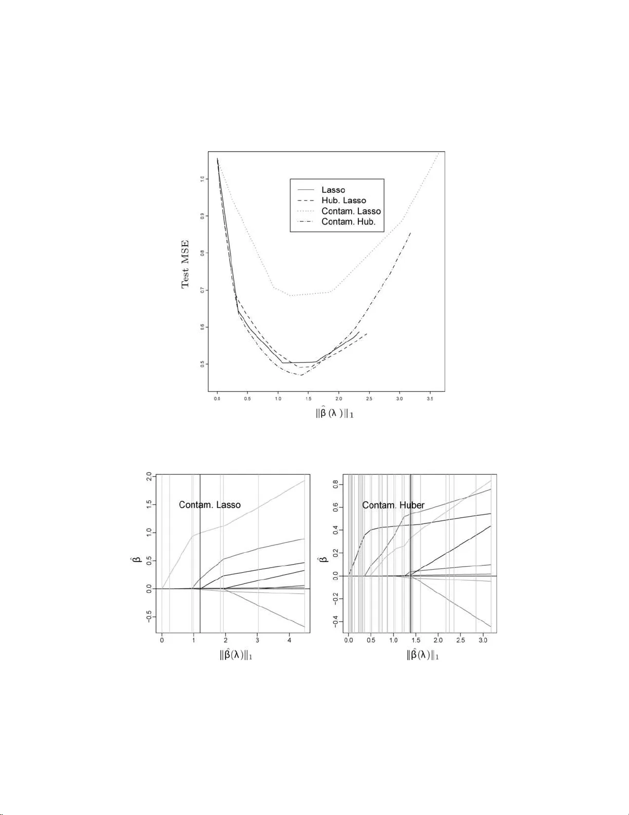
The Annals of Statistics 2007, V ol. 35, No. 3, 1012–10 30 DOI: 10.1214 /00905 3606000001370 c  Institute of Mathematical Statistics , 2007 PIECEWISE LINEAR REGULARIZE D SOLUTION P A THS By Saharon R osset and Ji Zhu 1 IBM T. J. Watson R ese ar ch Center and University of Michigan W e consider the generic regularized optimization problem ˆ β ( λ ) = arg min β L ( y , X β ) + λ J ( β ). Efron, Hastie, Johnstone and Tibshirani [ A nn. Statist. 32 (2004) 407–499] hav e show n th at for the LASSO— that is, if L is squared error loss a nd J ( β ) = k β k 1 is the ℓ 1 norm of β —the optimal co efficient path is piecewise li near, that is, ∂ ˆ β ( λ ) /∂ λ is piecewise constan t. W e derive a general character ization of t h e prop erties of (los s L , p enalt y J ) pairs which give piecewis e linear coefficient paths. S uch pairs allo w f or efficient generation of the full regularized coefficien t paths. W e in vestigate th e nature of efficient path follo wing algorithms which arise. W e use our results to sug- gest robust versions of the LASS O for regression and classification, and to deve lop new, efficien t algorithms for existing problems in the literature, i ncluding Ma mmen and v an de Geer’s lo cally adaptive re- gression splines. 1. In tro duction. Regularizati on is an essent ial component in mod ern data analysis, in particular when the num b er of predictors is large, p os- sibly large r than the num b er of observ ations, and nonregularized fitting is lik ely to giv e badly o ver-fitt ed and useless mo dels. In this p ap er w e consider the g eneric regularized optimizat ion problem. The inputs w e ha ve are: • A training data sample X = ( x 1 , . . . , x n ) ⊤ , y = ( y 1 , . . . , y n ) ⊤ , where x i ∈ R p and y i ∈ R for regression, y i ∈ {± 1 } for t w o-class classification. • A conv ex nonnegativ e loss functional L : R n × R n → R . • A con vex nonnegativ e p enalt y fu nctional J : R p → R , with J ( 0) = 0. W e will almost excl usiv ely use J ( β ) = k β k q in this pap er, that is, p enalizatio n of the ℓ q norm of the co efficien t v ector. Received S eptember 2003 ; revised June 2006 . 1 Supp orted b y NS F Gran t DMS-05-05432. AMS 2000 subje ct classific ations. Primary 62J07; secondary 62F35, 62G08, 62H30. Key wor ds and phr ases. ℓ 1 -norm p enalty, p olynomial spli nes, regulariza tion, solution paths, sparsit y , total v ariation. This is an electronic reprint of the orig inal article published by the Institute of Mathematical Statistics in The Annals of Statistics , 2007, V o l. 35, No . 3, 10 12–10 30 . This r e print differs from the original in pagination and typogra phic detail. 1 2 S. R OSSET AND J. ZHU W e wan t to find ˆ β ( λ ) = arg min β ∈ R p L ( y , X β ) + λJ ( β ) , (1) where λ ≥ 0 is the regula rization parameter; λ = 0 corresp onds to no regu- larizatio n, while lim λ →∞ ˆ β ( λ ) = 0. Man y of the commonly u sed m etho d s f or data mining, mac h ine learning and statistica l mo deling can b e describ ed as exact or approxima te regu- larized optimizati on approac hes. The ob vious examples from the statistics literature are explicit regularized linear r egression approac hes, suc h as ridge regression [ 9 ] and the LASSO [ 17 ]. Both of these use squared err or loss, but they differ in the p enalty they imp ose on the co efficien t v ector β : Ridge : ˆ β ( λ ) = min β n X i =1 ( y i − x ⊤ i β ) 2 + λ k β k 2 2 , (2) LASSO : ˆ β ( λ ) = min β n X i =1 ( y i − x ⊤ i β ) 2 + λ k β k 1 . (3) Another example from the statistics literature is the p enalized logist ic re- gression mo del for classification, whic h is w idely us ed in medical decision and credit scoring mo dels: ˆ β ( λ ) = min β n X i =1 log(1 + e − y i x ⊤ i β ) + λ k β k 2 2 . Man y “mo dern” metho ds f or mac h ine learning and signal pr o cessing can also b e cast in the framewo rk of regularized optimization. F or example, the regularized sup p ort v ector mac hine [ 20 ] uses the hinge loss function and the ℓ 2 -norm p enalt y: ˆ β ( λ ) = min β n X i =1 (1 − y i x ⊤ i β ) + + λ k β k 2 2 , (4) where ( · ) + is the p ositiv e part of the argument. Bo osting [ 6 ] is a p opular and highly successful metho d for iterativ ely b uilding an additiv e mo del from a dict ionary of “w eak learners.” In [ 15 ] we hav e sho wn that the AdaBo ost algorithm appr oximately follo ws the path of the ℓ 1 -regularized solutions to the exp onen tial loss fu nction e − y f as the regularizing parameter λ decreases. In this pap er, w e concen trate our atten tion on (loss L , p enalt y J ) pairings where the optimal p ath ˆ β ( λ ) is pie c ewise line ar as a fun ction of λ , that is, ∃ λ 0 = 0 < λ 1 < · · · < λ m = ∞ and γ 0 , γ 1 , . . . , γ m − 1 ∈ R p suc h that ˆ β ( λ ) = ˆ β ( λ k ) + ( λ − λ k ) γ k for λ k ≤ λ ≤ λ k +1 . Such mo dels are attractiv e b ecause they allo w us to generate th e whole regularized p ath ˆ β ( λ ) , 0 ≤ λ ≤ ∞ , simply b y sequ ential ly calculating the “step s izes” b et wee n eac h t w o consecutiv e λ PIECEWISE LIN EAR SOLUTIO N P A THS 3 v alues and the “directions” γ 1 , . . . , γ m − 1 . O ur discussion will concen trate on ( L , J ) pairs which al lo w efficien t generation of the w hole path and giv e statistic ally useful mo deling to ols. A canonical example is the LASSO ( 3 ). Recen tly [ 3 ] has shown that the piecewise linear co efficien t paths prop erty holds for the LASSO, and sug- gested the LAR–LASS O algorithm whic h tak es adv ant age of it. Similar algo- rithms were suggested for the LASSO in [ 14 ] and for total-v ariatio n p en alized squared error loss in [ 13 ]. W e hav e extended some p ath-follo wing ideas to v ersions of the regularized supp ort v ector mac h ine [ 7 , 21 ]. In this pap er, w e systemati cally in vesti gate the usefulness of piece wise linear solution paths. W e aim to com bine efficien t computational methods based on piecewise linear paths and stati stical considerations in suggest- ing new algorithms for exist ing regularized problems and in defining new regularized problems. W e tac kle three main questions: 1. What are the “families” of regularized problems that h a ve the piece- wise linear prop ert y? Th e general answer to this question is that the loss L has to b e a pie c ewise quadr atic function and the p enalt y J has to b e a pie c ewise line ar function. W e giv e some detail s and surv ey the resu lting “piecewise linear to olb o x” in Section 2 . 2. F or wh at m em b ers of these families can we design efficien t algo- rithms, either in the spirit of the LAR–LASSO algorithm or using differen t approac hes? Our main fo cus in this pap er is on d irect extensions of LAR– LASSO to “almost- quadratic” loss functions (Section 3 ) and to nonpara- metric regression (Section 4 ). W e briefly discuss some non-LAR t yp e results for ℓ 1 loss in Section 5 . 3. Out of the regularized problems we can th u s s olve efficien tly , whic h ones are of statistica l in terest? This can b e for t w o distinct reasons: (a) Regularized problems that are widely studied and used are obvio usly of interest , if we can offer n ew, efficien t algorithms for solving them. In this p ap er w e d iscuss in th is conte xt lo cally adaptive regression splines [ 13 ] (Section 4.1 ), quantil e r egression [ 11 ] and supp ort vect or mac h ines (Section 5 ). (b) Our efficien t algorithms allo w us to p ose s tatistic ally motiv ated reg- ularized pr oblems that h av e not b een considered in th e literature. In this con text, we prop ose robu st ve rsions of the LASSO for regression and classi- fication (Section 3 ). 2. The piecewise linear to olb ox. F or the co efficient paths to b e piece- wise linear, we require that ∂ ˆ β ( λ ) ∂ λ / k ∂ ˆ β ( λ ) ∂ λ k b e a piecewise constan t v ector as a fun ction of λ . Using T a ylor expansions of the normal equations for the min- imizing problem ( 1 ), w e can sh o w th at if L, J are b oth t wice d ifferen tiable 4 S. ROSSET AND J. ZHU in the neigh b orho o d of a solution ˆ β ( λ ), then ∂ ˆ β ( λ ) ∂ λ = − [ ∇ 2 L ( ˆ β ( λ )) + λ ∇ 2 J ( ˆ β ( λ ))] − 1 ∇ J ( ˆ β ( λ )) , (5) where we are using the n otatio n L ( ˆ β ( λ )) in the ob vious w ay , that is, w e mak e the dep endence on the data X , y (here assu med constan t) implicit. Pr oposition 1. A sufficient and ne c essar y c ond ition for the solutio n p ath to b e line ar at λ 0 when L, J ar e twic e differ entiable in a neighb orho o d of ˆ β ( λ 0 ) is that − [ ∇ 2 L ( ˆ β ( λ )) + λ ∇ 2 J ( ˆ β ( λ ))] − 1 ∇ J ( ˆ β ( λ )) (6) is a pr op ortional (i.e., c onstant up to multiplic ation by a sc alar) ve ctor in R p as a function of λ in a neighb orho o d of λ 0 . Prop osition 1 implies sufficient conditions f or p iecewise linearit y: • L is piecewise quadratic as a function of β along the optimal path ˆ β ( λ ), when X , y are assumed constan t at their sample v alues; and • J is p iecewise linear as a fun ction of β along this path. W e dev ote the rest of this pap er to examining some families of regularized problems whic h comply with these conditions. On the loss side, th is leads u s to consider fu nctions L which are: • Pure quadratic loss functions, like those of linear regression. • A mixture of quadratic and linear pieces, lik e Hub er’s loss [ 10 ]. These loss functions are of int erest b ecause they generate rob u st mo deling to ols. They will b e the fo cus of Section 3 . • Loss functions whic h a re p iecewise linear. These include sev eral w idely used loss fu nctions, lik e the h in ge loss of the su pp ort vect or mac hin e ( 4 ) and the c h ec k loss of quan tile r egression [ 11 ] L ( y , X β ) = X i l ( y i , β ⊤ x i ) , where l ( y i , β ⊤ x i ) =  τ · ( y i − β ⊤ x i ) , if y i − β ⊤ x i ≥ 0, (1 − τ ) · ( β ⊤ x i − y i ) , otherwise, (7) and τ ∈ (0 , 1) ind icates the qu antile of inte rest. On the p en alty side, our results lead u s to consider the ℓ 1 and ℓ ∞ p enalties as building b lo cks for piecewise linear solution paths. F or lac k of space, we limit the discussion in this pap er to the ℓ 1 p enalt y and its v ariant s (lik e total PIECEWISE LIN EAR SOLUTIO N P A THS 5 v ariatio n p enalties discussed in Sect ion 4 ). Results on the ℓ ∞ p enalt y can b e found in a full tec hnical rep ort on the second author’s homepage. ℓ 1 regularizatio n has several fa vorable statistical prop erties. Using ℓ 1 reg- ularization results in “sparse” solutions with a relativ ely small fraction of nonzero co efficient s, as opp osed to ℓ 2 regularizatio n wh ic h forces all n onzero co efficients [ 17 ]. In particular, if the num b er of predictors is larger than the n um b er of observ ations ( p > n ), then for any λ there exists an ℓ 1 -regularized solution with at most n nonzero co efficients [ 15 ]. Thus, in situations where the num b er of relev an t v ariables is small and there are a lot of irrelev an t “noise” v ariables, ℓ 1 regularizatio n ma y p ro ve far sup erior to ℓ 2 regulariza- tion from a prediction error p ersp ectiv e. F rom an inf erence/in terpretation p ersp ectiv e, ℓ 1 regularizatio n giv es “smooth” v ariable sele ction and m ore compact mo dels than ℓ 2 regularizatio n. In the case of orthogonal wa v elet bases, the soft thr esholding metho d p rop osed by [ 2 ], which is equiv alen t to ℓ 1 regularizatio n, is asymptotically nearly optimal (in a minimax sense) ov er a wide v ariet y of loss f unctions and estimated functions. It is n ot surprisin g, therefore, that ℓ 1 regularizatio n and its v arian ts h a ve b een widely and successfully used in differen t fields, including engineering and signal pr o cessing (suc h as basis pu rsuit and wa v elet thresholding), ma- c hine learning (suc h as b o osting and ℓ 1 SVM) and, obvi ously , statistics, where ℓ 1 and total v ariation p enalties are prev alen t. 3. Almost quadratic loss functions with ℓ 1 p enalt y . In this section, w e first define a f amily of “almost quadratic” loss f u nctions w hose ℓ 1 -p enalized v ersions generate p iecewise linear solution paths. W e formulate and prov e an algorithm, w hic h is an extension of the LAR–LASSO algorithm, that gener- ates the ℓ 1 -p enalized solution p aths for all memb ers of this family . W e then concen trate on t w o members of this family—Hub erized LASSO for regres- sion and ℓ 1 -p enalized Hub erized squared h in ge loss for classification—whic h define new, robu st, efficien t and adaptable mo d eling to ols. An R imple- men tation of these to ols is av ailable from the seco nd author’s homepage, www.stat.lsa.umic h.edu/˜jizh u /cod e/piecewise/ . 3.1. Main r esults. W e fix the p enalt y to b e the ℓ 1 p enalt y , J ( β ) = k β k 1 = X j | β j | , (8) and th e loss is required to b e differen tiable and piecewise quadratic in a fixed function of the sample resp ons e and the “prediction” β ⊤ x , L ( y , X β ) = X i l ( y i , β ⊤ x i ) , l ( y , β ⊤ x ) = a ( r ) r 2 + b ( r ) r + c ( r ) , (9) where r = ( y − β ⊤ x ) is the residual for regression and r = ( y β ⊤ x ) is the margin for classificatio n; and l ( r ) is a quadratic spline, that is, a ( · ) , b ( · ) , c ( · ) 6 S. ROSSET AND J. ZHU are p iecewise constan t fun ctions, defined so as to make the function l d iffer- en tiable. Some examples f r om this family are: • The squared error l ( y , β ⊤ x ) = ( y − β ⊤ x ) 2 , that is, a ≡ 1 , b ≡ 0 , c ≡ 0. • Hub er’s loss fun ction with fixe d knot t , l ( y , β ⊤ x ) =  ( y − β ⊤ x ) 2 , if | y − β ⊤ x | ≤ t , 2 t | y − β ⊤ x | − t 2 , otherwise. (10) • Squared hinge loss for classification, l ( y , β ⊤ x ) = (1 − y β ⊤ x ) 2 + . (11) Note that the hinge loss of the supp ort ve ctor mac hine and the chec k loss of quan tile regression d o not b elong to this family as they are not different iable at y β ⊤ x = 1 and y − β ⊤ x = 0, r esp ectiv ely . Theorem 2. Al l r e gularize d pr oblems of the form ( 1 ) using ( 8 ) , ( 9 ) (with r b eing ei ther the r esidual or the mar gin) gener ate pie c ewise line ar optimal c o efficient p aths ˆ β ( λ ) as the r e gularization p ar ameter λ varies. Pr oof. W e prov e th e theorem formally u sing the Karush –Ku hn–T uck er form u lation of the optimization problem. W e rewrite the regularized optimization problem as min β + ,β − X i l ( y i , ( β + − β − ) ⊤ x i ) + λ X j ( β + j + β − j ) sub ject to β + j ≥ 0 , β − j ≥ 0 ∀ j. The Lagrange primal function is X i l ( y i , ( β + − β − ) ⊤ x i ) + λ X j ( β + j + β − j ) − X j λ + j β + j − X j λ − j β − j . The deriv ativ es of th e pr imal and the corresp ond ing KKT conditions imply ( ∇ L ( β )) j + λ − λ + j = 0 , − ( ∇ L ( β )) j + λ − λ − j = 0 , λ + j β + j = 0 , λ − j β − j = 0 . Using these w e can figure that at the optima l solution for fixed λ the fol- lo wing scenarios should hold: λ = 0 ⇒ ( ∇ L ( β )) j = 0 ∀ j (unconstrained solution) , β + j > 0 , λ > 0 ⇒ λ + j = 0 ⇒ ( ∇ L ( β )) j = − λ < 0 ⇒ λ − j > 0 ⇒ β − j = 0 , β − j > 0 , λ > 0 ⇒ β + j = 0 (by similar reasoning) , | ( ∇ L ( β )) j | > λ ⇒ contradic tion. Based on these p ossible scenarios w e can see that: PIECEWISE LIN EAR SOLUTIO N P A THS 7 • V ariables can ha ve nonzero co efficien ts only if th eir “generalize d absolute correlatio n” |∇ L ( ˆ β ( λ )) j | is equal to λ . Thus, for eve ry v alue of λ we hav e a set of “activ e” v ariables A = { j : ˆ β j ( λ ) 6 = 0 } such that j ∈ A ⇒ |∇ L ( ˆ β ( λ )) j | = λ, sgn( ∇ L ( ˆ β ( λ )) j ) = − sgn( ˆ β ( λ ) j ) , (12) j / ∈ A ⇒ |∇ L ( ˆ β ( λ )) j | ≤ λ. (13) • When λ c hanges, the direction in whic h ˆ β ( λ ) is movi ng, that is, ∂ ˆ β ( λ ) ∂ λ , should b e suc h that it main tains the conditions ( 12 ), ( 13 ). So, if w e kn o w wh at the “activ e” set A is, it is a simple task to c h eck that as lo ng as we are in a r egion wh ere the loss is t wice differen tiable and the p enalt y is righ t differen tiable, w e will ha v e ∂ ˆ β ( λ ) A ∂ λ = − ( ∇ 2 L ( ˆ β ( λ )) A ) − 1 sgn( ˆ β ( λ ) A ) , (14) whic h is ju st a v ersion of ( 5 ), limited to only the activ e v ariables and sub- stituting the ℓ 1 p enalt y for J . F or the family of almost quadratic loss functions, we can deriv e ∇ 2 L ( ˆ β ( λ )) A explicitly , ∇ 2 L ( ˆ β ( λ )) A = X i 2 a ( r ( y i , ˆ β ( λ ) ⊤ A x A i )) x A i x ⊤ A i . Since a ( · ) is a piecewise constan t function, then ∇ 2 L ( ˆ β ( λ )) A and ∂ ˆ β ( λ ) A /∂ λ are also piecewise constan t; th erefore, the solution p ath ˆ β ( λ ) is piecewise linear. When one of the follo wing “ev ent s” o ccurs, t w ice differen tiabilit y is vio- lated and hence the direction in ( 14 ) will change: • Add a v ariable: A new v ariable should join A ; that is, w e reac h a p oin t where |∇ L ( ˆ β ( λ )) A C | ≤ λ will cease to hold if ˆ β ( λ ) k eeps mo ving in the same direction. • Drop a v ariable: A coefficien t in A hits 0. In that case, we reac h a n on- differen tiabilit y p oint in the p enalt y and w e can see that sgn( ∇ L ( ˆ β ( λ )) A ) = − sgn( β A ) will cease to h old if we conti n ue in the same direction. Thus w e need to drop the co efficien t hitting 0 from A . • Cross a knot: A “generalized r esidu al” r ( y i , ˆ β ( λ ) ⊤ x i ) hits a non-t wice differen tiabilit y p oint (a “knot”) in L , for example the “Hub erizing” p oint t in ( 10 ), or the hinge p oint 1 in ( 11 ). So we conclude that the path ˆ β ( λ ) w ill b e piecewise linear, with the direction giv en by ( 14 ) and direction c hanges occurring whenev er one of the three ev ents ab o ve happ ens . When it h app ens, w e need to up date A or a ( r ) to get a feasible scenario and recalculate the direction using ( 14 ).  8 S. ROSSET AND J. ZHU Based on the arguments in the pro of we can deriv e a generic algorithm to generate co efficien t paths for all mem b ers of the “almost quadratic” family of loss functions with ℓ 1 p enalt y . The LAR–LASSO algorithm [ 3 ] is a simplified v ersion of this algorithm since “knot crossing” ev ents do not o ccur in the LASSO (as the loss is twice d ifferentia ble). Our algorithm starts at λ = ∞ and follo ws the linear p ieces, while identifying the “ev en ts” and recalculating the direction when they o ccur. Algorithm 1. An algorithm for “almost quadratic” loss with ℓ 1 p enalt y . 1. Initialize: β = 0 , A = arg max j |∇ L ( β ) | j , γ A = − sgn( ∇ L ( β )) A , γ A C = 0 . 2. While (max |∇ L ( β ) | > 0): (a) d 1 = min { d > 0 : |∇ L ( β + dγ ) j | = |∇ L ( β + dγ ) A | , j / ∈ A } , d 2 = min { d > 0 : ( β + dγ ) j = 0 , j ∈ A} (h it 0), d 3 = min { d > 0 : r ( y i , ( β + dγ ) ⊤ x i ) hits a “knot,” i = 1 , . . . , n } . Find step length: d = min( d 1 , d 2 , d 3 ). (b) T ake step: β ← β + dγ . (c) If d = d 1 then add v ariable attaining equ alit y at d to A . If d = d 2 then remo ve v ariable attaining 0 at d from A . If d = d 3 for i ∗ , then assign n ew a ( r ( y i ∗ , β ⊤ x i ∗ )) from ( 9 ). (d) Calculate new direction: C = X i a ( r ( y i , β ⊤ x i )) x A ,i x ⊤ A ,i , γ A = C − 1 · sgn( β A ) and γ A C = 0 . It should b e noted that our formula tion here of the “a lmost quadratic” family with ℓ 1 p enalt y has ignored the existence of a nonp enalized in tercept. This has been done for simplicit y of exp osition, ho wev er incorp orating a nonp enalized in tercept in to the algorithm is straigh tforward. 3.2. Computationa l c onsider ations. What is the computational complex- it y of ru n ning Algorithm 1 on a d ataset w ith n observ ations and p v ariables? The ma jor computational cost for eac h step in volv es figur in g out the step length in (2a), and up dating the new d irection in (2d). The former tak es O ( np ) calc ulations, and the la tter requires O ( |A| 2 ) computations b y using in verse up d ating and do w ndating. It is difficult to p redict the num b er of steps on the solution p ath for arbitrary data. According to our exp erience, the total num b er of steps tak en PIECEWISE LIN EAR SOLUTIO N P A THS 9 b y the alg orithm is on a v erage O ( n ). T his can b e heur istically understo o d as follo ws. If n > p , it tak es O ( p ) steps to add all v ariables and O ( n ) steps for knot crossing; if n < p , since at most n v ariables are allo wed in the fitted mo del, it tak es O ( n ) steps for b oth add ing v ariables and crossing knots; the “drop even ts” are usually rare, O (1). Since the maxim um v alue of |A| is min( n, p ), it su ggests the ov erall computational cost is O ( n 2 p ). 3.3. The Hub erize d LASSO for r e gr ession. W e no w concen trate on t w o mem b ers of the “almost quadratic” family of loss functions—one for regres- sion and one for classificatio n. W e first consider the Hu b erized LASSO for regression. Th e loss is giv en b y ( 10 ). It is robust in the sense defined in [ 10 ], in that it protects against “con tamination” of the assumed n ormal errors. I t is “almost quadr atic” as defined in Sectio n 3.1 , and so T heorem 2 and Algorithm 1 apply to its ℓ 1 regularized solution paths. Pr ostate c anc er dataset. W e use the “prosta te cancer” dataset [ 17 ] to compare the pr ediction p erformance of the Hu b erized LASSO to th at of the LASSO on the original d ata and after w e artificially “con taminate” the data b y adding large constan ts to a small n um b er of resp onses. W e used the training-test split as in [ 8 ]. The training set consists of 67 observ ations and the test set of 30 observ atio ns. W e r an the LASSO and the Hub erized LASSO w ith a knot a t t = 1 on the original dataset, and on the “con taminated” dataset where 5 has b een added/su b tracted to the resp onses of 12 observ ations. Figure 1 sh o ws the mean squ ared error on the 30 test set observ ations for the four resulting regularized solution paths from solving the LASSO and Hub erized LASS O for all p ossible v alues of λ on the t wo datasets. W e ob- serv e that on the n oncon taminated data, the LASS O (solid) and Hub erized LASSO (dashed) p erform quite similarly . When w e add conta mination, the Hub erized LASSO (dash-dotted) do es not s eem to suffer from it at all, in that its b est te st set p erform ance is comparable to that of b oth r egular- ized mo dels on the n oncon taminated d ata. The prediction p erformance of the standard LASSO (dotted), on the other hand, deteriorates s ignifican tly ( t -test p -v alue 0 . 045) when cont amination is added, illustrating the lac k of robustness of squared error loss. The tw o LASSO solutions con tain n ine linear pieces eac h, while the Hub er- LASSO path for the noncon taminated d ata conta ins 41 p ieces, and the one for the conta minated data con tains 39 pieces; b oth agree with our conjecture in Section 3.2 th at the num b er of steps is O ( n ) . Figure 2 sho ws the solution paths for the con taminated LASS O mo del and the cont aminated Hub er- LASSO mo del. W e observe that the t w o paths are quite different and the t wo b est m o dels (corresp ond in g to the solid v ertical lines) are also different. 10 S. ROSSET AND J. ZHU Fig. 1. T est M SE of the mo dels along the r e gularize d p aths. Se e text f or details. Fig. 2. Solution p aths of the LASSO ( left ) and th e Hub erize d LASSO ( right ) on the c ontaminate d pr ostate c anc er tr aining data. The vertic al gr ey lines c orr esp ond to the steps along the solution p aths. The vertic al solid lines c orr esp ond to the mo dels that give the b est p erformanc es on the test data. PIECEWISE LIN EAR SOLUTIO N P A THS 11 Fig. 3. R e gularize d p aths and pr e diction err ors for the lo gistic loss ( left ) , Hub erize d squar e d hinge l oss ( midd l e ) and squar e d hinge loss ( right ) . The lo gistic loss and the Hu- b erize d squar e d hinge l oss ar e b oth less affe cte d by the outlier. 3.4. The Hub erize d squ ar e d hinge loss for classific ation. F or classification w e would lik e to ha v e a loss wh ich is a function of the margin, r ( y , β ⊤ x ) = ( y β ⊤ x ). This is true of all loss fun ctions t ypically used for classificati on, lik e the negativ e binomial log-lik eliho o d for logistic r egression, the h inge loss for the sup p ort ve ctor mac hine and exp onen tial loss for b o osting. Th e prop erties w e w ould lik e from our classification loss are: • W e would lik e it to b e “almost quadr atic,” so we can apply the Algorithm 1 in Section 3.1 . • W e would lik e it to b e robust, that is, linear for large abs olute v alue negativ e margins (lik e the logi stic or hinge), so that outl iers will h a ve a small effect on the fit. This leads u s to suggest for classification the “Hub erized squared hinge loss,” that is, ( 11 ) “Hub erized” at t < 1, l ( y , β ⊤ x ) =    (1 − t ) 2 + 2( 1 − t )( t − y β ⊤ x ) , if y β ⊤ x ≤ t , (1 − yβ ⊤ x ) 2 , if t < y β ⊤ x ≤ 1, 0 , otherwise. (15) 12 S. ROSSET AND J. ZHU It is a simple task to sho w that arg min f E y l ( y , f ) = 2 Pr( y = 1) − 1 . Hence the p opulation minimizer of the Hub erized squared hinge loss giv es the correct sign for classification. T o illustrate the robustness of this loss ( 1 5 ) and its computational su- p eriorit y ov er the logistic loss, we considered the follo wing simple example: x ∈ R 2 with class cente rs at ( − 1 , − 1) (class “ − 1”) and (1 , 1) (class “1”) with one big outlier at (30 , 100) b elonging to the cl ass “ − 1.” Th e Ba y es mod el, ignoring the outlier, is to classify to class “1” if and only if x 1 + x 2 > 0. Figure 3 sho ws the regularized solution paths and misclassificati on rate for this example using the logi stic loss (l eft), the Hub erized squared hinge loss (middle) and the squared hinge loss (righ t), all with ℓ 1 p enalt y . W e observ e that the logistic and Hu b erized regularized mo del p aths are b oth less affe cted b y the outlier than the non-Hub erized squared loss. Ho wev er, logistic loss d o es not allo w for efficien t calculation of the ℓ 1 regularized path. 4. Nonparametric regressio n, total v ariatio n p enalties and piec ewise lin- earit y . T otal v ariation p enalties and closely asso ciated sp line metho ds for nonparametric regression hav e exp erienced a surge of inte rest in the statistics literature in recent ye ars. The tota l v ariation of a univ ariate differen tiable function f ( x ) is TV dif ( f ) = Z ∞ −∞ | f ′ ( x ) | dx. If f is nondifferentia ble on a coun table set x 1 , x 2 , . . . , then TV ( f ) is the sum of TV dif ( f ), calculate d ov er the differenti able set only and the absolute “jumps” in f where it is noncon tin uous . In what f ollo ws we assume the range of f is limited to [0 , 1]. T otal v ariation p enalties tend to lead to regularized s olutions wh ic h are p olynomial splines. [ 13 ] in vest igates the solutions to total-v ariat ion p enalized least squ ares pr oblems. The authors use total v ariation of ( k − 1)st ord er deriv ativ es, n X i =1 ( y i − f ( x i )) 2 + λ · TV ( f ( k − 1) ) . (16) They sh o w that there alw ays exists a solution ˆ f k ,λ suc h that ˆ f ( k − 1) k ,λ is p iece- wise constan t, that is, ˆ f k ,λ is a p olynomial s p line of ord er k . F or k ∈ { 1 , 2 } the knots of the spline solutions are guaran teed to b e at the data p oint s. A similar setup is considered in [ 1 ]. Their taut-string and lo c al squ e ezing metho ds lead to solutions that are p olynomial splines of d egree 0 or 1, with knots at data p oints. PIECEWISE LIN EAR SOLUTIO N P A THS 13 No w, consider a p olynomial spline f of order k , with h knots lo cated at 0 < t 1 < · · · < t h < 1, that is, f ( x ) = h X j = 1 β j ( x − t j ) k − 1 + + q ( x ) , (17) where q ( x ) is a p olynomial of degree k − 1. The total v ariation of the ( k − 1)st deriv ativ e of f clearly corresp ond s to an ℓ 1 norm of the set of co efficients of the appropriate spline basis functions, anc h ored at the knots, TV ( f ( k − 1) ) = ( k − 1) ! · h X j = 1 | β j | . (1 8) If the knots t 1 , . . . , t h are fixed in adv ance (e.g., at the d ata p oints) , then a total v ariation p enalized problem is equiv alen t to an ℓ 1 -p enalized r egression problem, with p = h d eriv ed predictors. If w e also emp lo y squared error loss, w e get a LASSO problem, and w e can use the LAR–LASSO algorithm to compute the complete regularized solution path. T he only difference from the standard LAS S O is the existence of k nonp enalized co efficien ts for the p olynomial q ( x ), instead of the interce pt only f or the LASSO. This requires only a slight mo d ification to the LAR–LASSO algorithm. Th is leads to es- sen tially the same algorithm as Algorithm 2 of [ 13 ] for finding the regularized path for an y k w ith a fixe d, pr e determine d set of candidate kn ots. 4.1. L o c al ly adaptive r e gr ession splines. W e no w concen trate on the fam- ily of p enalized problems ( 16 ) defined by Mammen and v an de Geer [ 13 ]. As we hav e men tioned, [ 13 ] dev elops an exact metho d for finding ˆ f k ,λ when k ∈ { 1 , 2 } and appr oximate metho ds for k > 2 (where the kn ots of the op- timal solutions are not guaran teed to b e at the data p oin ts). W e no w show ho w we can u s e our app roac h to fin d the spline solution ˆ f k ,λ exactly for an y natural k . The resulting alg orithms get p ractical ly more complicated as k increases, but their theoretical computational complexit y remains fixed. When the knots are not guarant eed to b e at the data p oin ts, we can still write the total v ariation of p olynomial splines as the sum of ℓ 1 norms of co efficients of basis fu nctions, as in ( 18 ). How ev er, we do not h a ve a finite predefined set of candidate basis functions. Rather, we are dealing with an infinite set of candidate basis functions of the form X = { ( x − t ) k − 1 + : 0 ≤ t ≤ 1 } . Our algorithm for tracki ng the regularized solution p ath ˆ f k ,λ in this case pro ceeds as follo ws. W e start at the solution for λ = ∞ , whic h is the least squares ( k − 1)st degree p olynomial fit to the data. Giv en a solution ˆ f k ,λ 0 for some v alue of λ 0 , wh ic h includes n λ 0 knots at t 1 , . . . , t n λ 0 , d enote z ( x ) = (1 , x, x 2 , . . . , x k − 1 , ( x − t 1 ) k − 1 + , . . . , ( x − t n λ 0 ) k − 1 + ) ⊤ , 14 S. ROSSET AND J. ZHU whic h is the curren t predictor v ector. F ollo wing ( 17 ) we can write ˆ f k ,λ 0 ( x ) = ˆ β ( λ 0 ) ⊤ z ( x ) . F ollo wing the logic of the LAR–LASSO algorithm, we see that the solution will c han ge as ˆ f k ,λ 0 − d = ( ˆ β ( λ 0 ) + dγ ) ⊤ z ( x ) , where γ = − ( k − 1)! · ( Z ⊤ Z ) − 1 · s , Z = ( z ( x 1 ) , . . . , z ( x n )) ⊤ and s ∈ R k + n λ 0 is a vect or with 0 comp onen ts corresp ond ing to 1 , x, . . . , x k − 1 and ± 1 com- p onent s corresp onding to eac h ( x − t j ) k − 1 + [with the sign b eing th e opp osite of the sign of ( x − t j ) k − 1 ⊤ + ( y − ˆ f k ,λ 0 )]. What we n o w need to id entify is the v alue of λ at whic h an additional kn ot needs to b e added, and the lo cation of that knot. Consid er fi r st a fixed kn ot candidate t . Th en we can see that the LAR–LASSO criterion for add ing this kn ot to the set of “activ e” kn ots is | x ⊤ t ( y − Z ˆ β ( λ 0 ) − ( λ 0 − λ ) Z γ ) | = λ, where x t = ( x − t ) k − 1 + (column v ector of length n ). More explicitly , define λ + ( t ) = x ⊤ t ( y − Z ˆ β ( λ 0 ) − λ 0 Z γ ) 1 − x ⊤ t Z γ , (19) λ − ( t ) = x ⊤ t ( y − Z ˆ β ( λ 0 ) − λ 0 Z γ ) − 1 − x ⊤ t Z γ . (20) Then we can write λ ( t ) =  max( λ + ( t ) , λ − ( t )) , if max( λ + ( t ) , λ − ( t )) ≤ λ 0 , min( λ + ( t ) , λ − ( t )) , if m ax ( λ + ( t ) , λ − ( t )) > λ 0 . (21) No w w e see that w e can in f act let t b e a parameter and find the next knot to b e added to the optimal solution path by maximizing λ ( t ), that is, λ add = max t ∈ (0 , 1) \{ t 1 ,...,t n λ 0 } λ ( t ) , (22) whic h is the v alue of λ where we stop mo ving in d irection γ , add a knot at the argumen t of the maxim u m and recalculate the direction γ . Solving ( 22 ) requires find ing the lo cal extrema of the functions in ( 21 ), whic h are rational fu nctions within eac h int erv al b etw een t wo p oin ts which are either data p oin ts or knots (with n umerator and denominator b oth of degree k − 1). Thus, a r easonable tactic is to fin d the extrema w ithin eac h suc h in terv al, then compare them b etw een the int erv als to find the o ve rall solution to ( 22 ). F or sm aller v alues of k it can b e solve d manual ly and exactly: PIECEWISE LIN EAR SOLUTIO N P A THS 15 • F or k ∈ { 1 , 2 } , w e get a ratio of co nstan t or linear functions in ( 21 ), and therefore the extrema—and the knots—are guarante ed to b e at the data p oin ts, leading to the algorithm of [ 13 ]. • F or k = 3 we get a r atio of quadratics in ( 21 ), and we can find the extrema within eac h segmen t analytical ly . These extrema ma y not corresp ond to the segment’ s end p oin ts, and so we ma y hav e knots that are not at data p oin ts. Assuming w e ha v e the co de to solv e the maximization problem in ( 22 ), Algorithm 2 giv es a general sc h ema f or follo w ing the solution path ˆ f k ,λ for an y v alue of k . Algorithm 2. T rac kin g the path of TV-p enalized solutions. 1. Initialize: f ( x ) = (1 , x, . . . , x k − 1 ) ⊤ β ls is the LS p olynomial fit of degree k − 1 , u = arg max t ∈ (0 , 1) | ( x − t ) k − 1 ⊤ + ( y − f ( x )) | (assumed u nique) , T = { u } , λ 0 = ( k − 1)! · | ( x − u ) k − 1 ⊤ + ( y − f ( x )) | , Z = ( 1 , x , . . . , x k − 1 , ( x − u ) k − 1 + ) , ˆ β ( λ 0 ) = ( β ⊤ ls , 0) ⊤ , s = ( 0 ⊤ k , − sgn { ( x − u ) k − 1 ⊤ + ( y − f ( x )) } ) ⊤ . 2. While P i ( y i − f ( x i )) 2 > 0: (a) Set γ = − ( k − 1)!( Z ⊤ Z ) − 1 s . (b) ∀ t ∈ (0 , 1) \ T d efi n e λ + ( t ) , λ − ( t ) , λ ( t ) as in ( 19 )–( 21 ). (c) Solv e the maxim u m problem in ( 22 ) to get λ add . (d) Let λ rem = λ 0 − min { d > 0 : ∃ j > k s.t. ˆ β j ( λ 0 ) + dγ j = 0 } . (e) If λ add > λ rem add a knot at the p oin t attaining the maxim um in ( 22 ), and up d ate T , Z and s . (f ) Similarly , if λ add < λ rem remo ve th e knot attaining 0 at λ rem . (g) In b oth cases, up d ate: ˆ β ( λ 0 ) ← ˆ β ( λ 0 ) + ( λ 0 − max( λ add , λ rem )) γ , λ 0 ← max( λ add , λ rem ) . Since we can neve r ha ve more than n − k knots in a solution ˆ f k ,λ [ 15 ], the computational complexit y of eac h iteration of the algorithm is b oun ded at O ( n 2 ) calculations for finding the next kn ot and O ( n 2 ) for calculating the next direction (us in g up dating form u las). The num b er of steps of the algorithm is difficult to b oun d, b ut fr om our exp erience seems to b ehav e like O ( n ) (wh ic h is the conjecture of [ 13 ]). 16 S. ROSSET AND J. ZHU Fig. 4. Applying Algorith m 2 ( w i th k = 3 ) to a data example wher e the underlying curve is a quadr atic spli ne with knots at 0 . 25 , 0 . 5 and 0 . 75 . Se e text for details. 4.2. Simple data example : k = 3 . W e illustrate our algorithm on a simp le data example. W e select 100 x samples uniformly on (0 , 1). W e d ra w the corresp onding y v alues as N ( g ( x ) , 0 . 03 2 ), where g ( x ) is a p olynomial s pline with knots at 0 . 25 , 0 . 5 and 0 . 75, g ( x ) = 0 . 125 + 0 . 125 x − x 2 + 2( x − 0 . 25 ) 2 + − 2( x − 0 . 5) 2 + + 2( x − 0 . 75) 2 + . g ( x ) is plotted as the solid line in Figure 4 , and the noisy y v alues as circles. The signal-to-noi se ratio is ab out 1 . 4. W e app ly our Algorithm 2 with k = 3 . Figure 4 s ho ws the r esu lting mo dels after 5, 15 and 50 iterat ions of the algorithm. After 5 iterat ions, the r egu- larized spline con tains three knots lik e the true g , bu t these are all around 0 . 5. The fitted mo del, dra wn as a d ashed cur v e, is clearly underfitted. The corresp onding reducible squared prediction error is 9 . 5 × 10 − 4 . PIECEWISE LIN EAR SOLUTIO N P A THS 17 After 15 iterations, the sp line con tains four kn ots, at 0.225, 0.255, 0.485 and 0 . 755. The fir st one h as a small co efficien t, and the other three closely corresp ond to the knots in g . The resulting fit (dotted curv e) is a reasonable appro ximation of g , and the reducible squared error is ab out 3 . 1 × 10 − 4 . After 50 iterations the m o del cont ains ten knots and the data is clearly o ve rfitted (dash-dotted curv e, reducible squared error 8 . 2 × 10 − 4 ). Although the algorithm should in principle con tinue until it interp olates the data, in practice it terminates b efore (in this case after ab out 180 itera- tions) and is n umerically unable to further impr ov e the fit. This is analogous to the situation describ ed in [ 7 ] for ke rnel SVM, w h ere the effectiv e rank of the kernel m atrix is significant ly smaller than n , since many eigen v alues are effectiv ely zero. 5. Using ℓ 1 loss and its v ariants. Pie cewise linear nondifferent iable loss functions app ear in practice in b oth regression and classification problems. F or regression, absolute v alue loss v arian ts lik e the qu an tile regression loss are qu ite p opular [ 11 ]. F or classification, the hinge loss is of great imp ortance, as it is the loss underlying the su pp ort v ector mac hine [ 20 ]. Here w e consider a generalized formulati on, w h ic h co v ers b oth of ( 7 ) and ( 4 ). The loss function has the form l ( r ) =  b 1 · | a + r | , if a + r ≥ 0, b 2 · | a + r | , if a + r < 0, (23) with the generalized “residu al” b eing r = ( y − β ⊤ x ) for r egression and r = ( y · β ⊤ x ) for classification. When these loss functions are com bined with ℓ 1 p enalt y (or total v ariation p enalt y , in appropr iate f u nction classes [ 12 ]), the resulting regularized p r ob- lems can b e formulated as linear pr ogramming p roblems. When the path of regularized solutions ˆ β ( λ ) is considered, it turns out to hav e in teresting structure with regard to λ : Pr oposition 3. F or loss functions of the form ( 23 ) , ther e exists a set of values of the r e gularization p ar am eter 0 < λ 1 < · · · < λ m = ∞ such that : • The solution ˆ β ( λ k ) is not uniqu e ly define d, and the set of optimal solutions for e ach λ k is a str aight line in R p . • F or any λ ∈ ( λ k , λ k +1 ) , the solution ˆ β ( λ ) is fixe d and e q u al to the min- imum ℓ 1 norm solution for λ k and the maximum ℓ 1 norm solution for λ k +1 . Prop osition 3 generalizes observ ations on the path of s olutions made in the con text of quantile regression in [ 12 ] and in the con text of 1 -norm sup p ort v ector machines in [ 21 ]. Note that this leads to d escribin g a r egularized path 18 S. ROSSET AND J. ZHU whic h is pie c ewise c onstant as a function of the regularization p arameter λ , with j umps at the v alues λ 1 , . . . , λ m . Ho wev er, it is still pie c ewise line ar in the ℓ 1 norm of the soluti on, k ˆ β ( λ ) k 1 . The alg orithm for computing the solution path follo ws the spirit of our earlier wo rk [ 21 ]. F or brevit y we omit the details. W e note, h o wev er, that it is fund amen tally differ ent from the LARS–LASSO algorithm and Algorithm 1 , b ecause we are now d ealing with a nondifferent iable loss function. An in teresting v ariant of piecewise linea r loss is to replace the ℓ 1 loss with an ℓ ∞ loss, wh ic h is also p iecewise linear and nondifferent iable. It leads to in teresting “mini-max” estimat ion pro cedur es, p opu lar in man y areas, including engineering and con trol. F or example, [ 19 ] p rop oses the use of ℓ 1 - p enalized ℓ ∞ -loss solutions in an image reconstruction problem (b ut do es not consider th e solution path). P ath-follo w ing algorithms can b e d esigned in the same spirit as the ℓ 1 loss case. 6. Conclusion. In this pap er w e com bine computational and statistical considerations in designing regularize d modeling to ols. W e emp h asize the imp ortance of b oth appropr iate regularization and robust loss functions for successful practical mo d eling of data. F rom a statistica l p ersp ectiv e, w e can consider robustness and regularization as almost ind ep endent desirable pr op- erties dealing with different issues in predictiv e mo deling: • Robustness mainly protects u s against wrong assumptions ab out our error mo del. It d o es little or nothing to protect us against the uncertain ty ab out our mo d el structure whic h is inh eren t in the fin iteness of our data. F or example, if our errors r eally are normal, then squared err or loss minimizes the asymptotic v ariance of th e coefficien ts, no matter h o w lit tle data w e ha ve or ho w inapp r opriate our mo del is [ 10 ]. Using robust loss in su c h a situation is always coun ter-pro d uctiv e. • Regularization deals mainly with the un certain t y ab out our p redictiv e mo del structure b y limiting the mo del sp ace. Note, in this con text, the equiv alence b et ween the “p enalized” f orm u lation ( 1 ) and a “constrained” form u lation min β L ( y , X β ) sub j ect to J ( β ) ≤ s . The tw o form u lations share the same solution path. The constrained formulati on exp oses the goal of regularizatio n as “simplifying” the mo del estimation problem b y limiting the set of considered m o dels. There are man y inte resting directions in which our work can b e extended. W e m a y ask, how can our geometric understanding of the regularized solu- tion paths h elp us to analyz e the statistical prop erties of the mo dels along the path? F or exa mple, [ 3 ] h as offered analysis of the LASS O p ath. This b ecomes m u c h m ore c h allenging once w e stray a wa y fr om s quared error loss. W e may also consider more complex p enalt y structure, su c h as lo cal or d ata- dep endent p enalties [ 1 ] or multiple p enalties [ 18 ]. PIECEWISE LIN EAR SOLUTIO N P A THS 19 Finally , it is w orth noting that limiting our d iscus s ion to con vex p roblems, for whic h efficien t algorithms can b e designed, lea v es out some other statisti- cally we ll m otiv ated fitting approac h es. The use of a noncon vex p enalt y was adv o cated b y F an and collab orators in several pap ers [ 4 , 5 ]. Th ey exp ose the fav orable v ariable selectio n pr op ert y of the p enalt y fun ction they offer, whic h can b e viewed as an imp ro vemen t o ver the use of ℓ 1 p enalt y . [ 16 ] ad- v o cates the use of n onconv ex ψ -loss in the classification s etting, minimizing the effect of outliers and misclassified p oint s. Th is approac h can b e view ed as an ev en m ore robus t versio n of our Hub erized loss fu nction, with strong statistic al motiv atio n in terms of asymptotic b ehavio r. Ac kn o wledgment s. W e thank the referee, Asso ciate Ed itor and Co-Editors J. F an and J. Marden for their thought ful and useful commen ts, and in par- ticular for introducing us to th e relev an t literature on total v ariation p enal- ties. W e thank B. Efron, J. F riedman, T. Hastie, R. Tibsh irani, B. Y u and T. Zhang for their helpful commen ts and suggestions. REFERENCES [1] Da vi es, P. L. and Ko v ac, A . (2001). Lo cal extremes, run s, strings and multireso- lution ( with d iscussion). Ann. Statist. 29 1–65. MR183395 8 [2] Donoho, D. , Johnstone, I., Kerky a charian, G . and Picard, D. (1995). W a velet shrink age: Asympt opia? (with discussion). J. R oy. Statist. So c. Ser. B 57 301– 369. MR132334 4 [3] Efr on, B., Ha stie, T., Johnstone, I. M. and Tibshirani, R. (2004). Least angle regressio n (with discussion). Ann. Statist. 32 407–499. MR206016 6 [4] F an, J. and Li, R. (2001). V aria ble selection v ia nonconcav e p enalized lik elihoo d and its oracle prop erties. J. Amer. Statist. Asso c. 96 1348–136 0. MR194658 1 [5] F an, J. and Peng, H. (200 4). Nonconca ve p enalized likelihoo d with a diverging num b er of parameters. Ann. Statist. 32 928–961. MR206519 4 [6] Freund, Y. and Schapi re, R. E. (1996). Exp eriments with a n ew b oosting algo- rithm. In Pr o c. 13th International Confer enc e on Machine L e arning 148– 156. Morgan K auffman, S an F rancisco. [7] Hastie, T., R osset, S., Tibshirani, R. and Zhu, J. (2004). The entire regulariza- tion p ath for the supp ort vector mac hine. J. Mach. L e arn. R es. 5 1391–1415. [8] Hastie, T., T ibshirani, R. and Friedman, J. (2001). The Elements of Statis- tic al Le arning : Data Mi ning , Infer enc e and Pr e di ction . Sp ringer, New Y ork. MR185160 6 [9] Hoerl, A. and Kennard, R. (1970). R idge regression: Biased estimation for nonorthogonal p roblems. T e chnomet rics 12 55–67. [10] Huber, P. (1964). R obu st estimation of a location parameter. Ann. Math. Statist. 35 73–101. MR016141 5 [11] Koenker, R. (2005). Quantile R e gr ession . Cambridge U niv. Press. MR2268657 [12] Koenker, R., Ng, P. and Por tno y, S. (1994). Quantile smoothing splines. Biometrika 81 673–680. MR132641 7 [13] Mammen, E. and v an de Gee r, S. (1997). Lo cally adaptive regression splines. Ann. Statist. 25 387–413. MR142993 1 20 S. ROSSET AND J. ZHU [14] Osborne, M., Presnell, B. and Turlach, B. (2000). On the LASS O and its dual. J. Comput. Gr aph. Statist. 9 319– 337. MR182208 9 [15] Rosset, S ., Zhu, J. and Ha stie, T. (2004). Boosting as a regularized path to a maxim um margin classifier. J. M ach. L e arn. R es. 5 941–973. [16] Shen, X., Tse ng, G., Zhang, X. and W ong, W. H. (200 3). On ψ -learning. J. Amer . Statist. Asso c. 98 724–734 . MR2011686 [17] Tibshirani , R. (1996). R egression shrink age and selection via t he lasso. J. R oy. Statist. So c. Ser. B 58 267–288. MR137924 2 [18] Tibshirani , R. , Saunders, M., Ross et, S ., Zhu, J. and Knight, K. (2005). Spar- sit y and smo othness v ia the fused lasso. J. R . Stat. So c. Ser. B Stat. Metho dol. 67 91–108. MR213664 1 [19] Tsuda, K. and Ra tsch, G. (2005). I mage reconstruction by linear p rogramming. IEEE T r ans. Image Pr o c ess. 14 737–74 4. [20] V apnik, V. (199 5). The Natur e of Statistic al L e arning The ory . Springer, New Y ork. MR136796 5 [21] Zhu, J., R osset. S ., Hastie, T. and Tibshira ni, R. (2003). 1-norm supp ort vecto r mac hines. In A dvanc es in Neur al Information Pr o c essing Systems 16 . Predictive Modeling Group IBM T. J. W a tson Research Center Yorktow n Heights, New York 10 598 USA E-mail: srosset@us.ibm.com Dep ar tment of St a tistics University of Michigan 1085 South University Ann Arbor, Michigan 48109 USA E-mail: jizhu@umic h.edu