Diversity of MIMO Multihop Relay Channels - Part I: Amplify-and-Forward

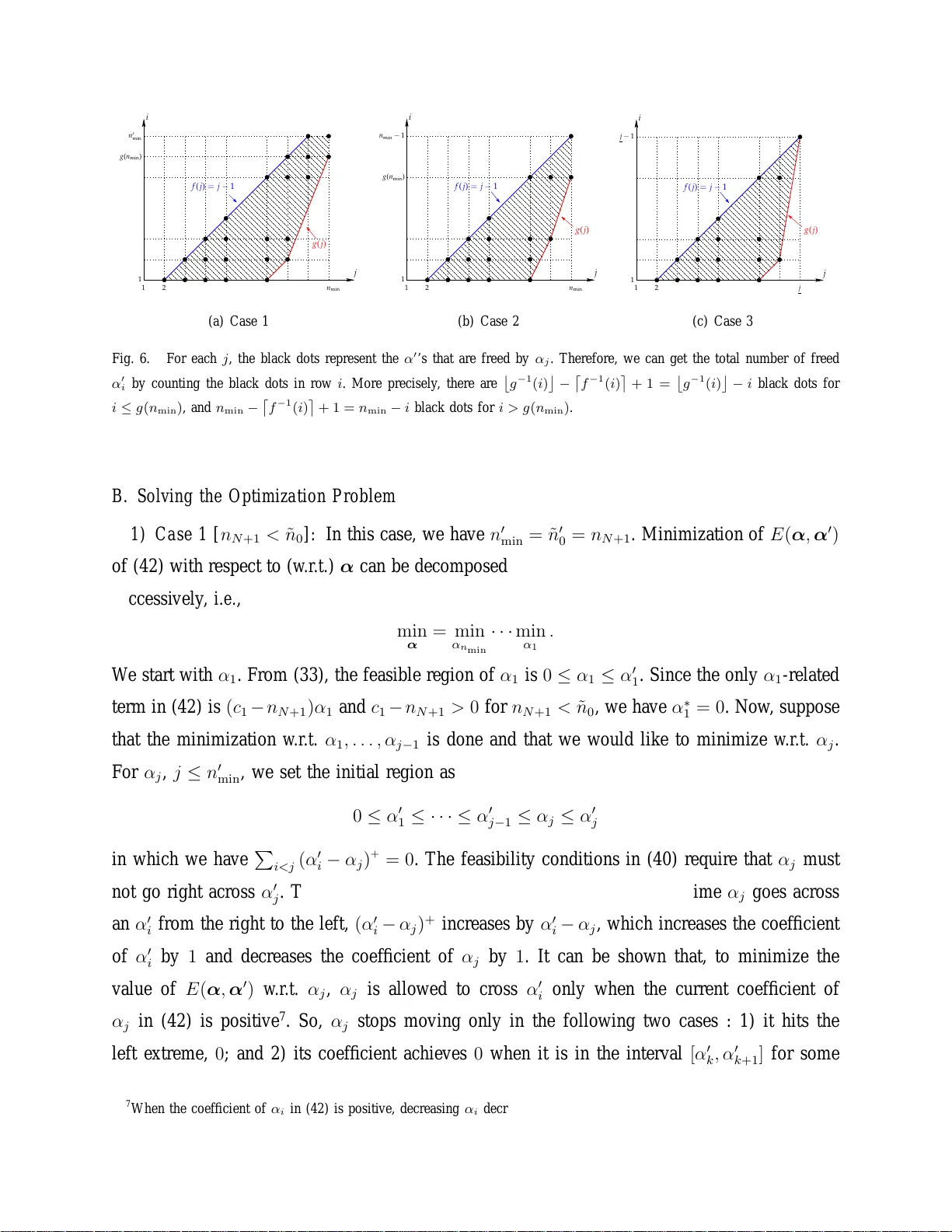
Di v ersity of MIMO M ultihop Relay Channels—P art I: Amplif y-and-F orwar d Sheng Y ang and Jean-Claude Be lfiore Abstract In this two-part paper, we consider the multiantenna multihop relay chan nels in which the source signal ar riv es at the destination th rough N indepen dent relaying ho ps in series. The main concer n of this work is to design relay ing strategies that utilize efficiently the relay s in such a way that th e div ersity is maximized. In part I, we fo cus on the am plify-and -forward (AF) strategy with which the relays simply scale the r eceiv ed signal and retransmit it. More specifically , we characterize the diversity-multiplexing tradeoff (DMT) of th e AF schem e in a general multiho p channel with arbitrary number of antennas and arbitr ary n umber of hops. The DMT is in clo sed-form expression as a function of the num ber of antennas at each no de. First, we provide some basic results on the DMT of the g eneral Rayleigh produ ct channels. I t tur ns ou t that these results hav e very simple and intuiti ve interpr etation. Then , the results are applied to the AF multihop channels which is shown to be equivalent to th e Rayleigh p roduct channel, in the DMT sense. Finally , the project-and- forward (PF) sche me, a variant of the AF schem e, is proposed. W e sh ow that th e PF scheme has the same DMT as the AF scheme, while the PF can have significant po wer gain over the AF scheme in some cases. In par t II, we will der iv e the u pper bou nd on the div ersity of the m ultihop channe ls and show that it can be achieved by partitioning the multihop channel into AF sub channels. Index T erms Multihop, multiple-input multiple output (MIMO), relay channel, amplify-and-fo rward (AF), di versity- multiplexing trad eoff (DMT). Manuscript submitted to the IEEE T ransactions on Information Theory . The authors are with the Departmen t of Commu- nications and Electronics, ´ Ecole Nationale Sup ´ erieure des T ´ el ´ ecommunications, 46, rue Barrault, 7501 3 Paris, France (e-mail: syang@enst.fr; belfiore@enst.fr). October 22, 2021 DRAFT 1 Di v ersity of MIMO M ultihop Relay Channels—P art I: Amplif y-and-F orwar d I . I N T RO D U C T I O N A N D P RO B L E M D E S C R I P T I O N W ireless relaying system s have lots of advantages over tradit ional direct transmission sy stems. For e xample, the periphery can be e xtended by the re lays and the co verage of the e x isting netw ork can be improve d. Using relays can also shorten th e point to point transmis sion distance, which results i n lower power (interference) lev el or in high er throughput . Furthermore, all these b enefits can be realized in a more fle xible, easier and cheaper t o deploy network. Recently , t here has been a boosting interest in the cooperative d iv ersity w ith which the spatial div ersity is exploited through distributed relays. Since the work of Sendonaris et al. [1], [2] that introd uced the notio n of cooperativ e diver sity , a number of relaying protocols hav e been proposed (see, e.g. , [3]–[10]). Most of the previous works consi der th e singl e-antenna two-hop relay channel where the source signal i s abl e to arrive at the dest ination t hrough at most two hops, i.e. , the source-relay hop and relay-destination hop. In an N -relay channel, i t is shown that a diversity order of N + 1 (respectively , N ) can be achie ved with (respecti vely , wit hout) the direct source-destin ation link. In this work, we consi der the MIMO mult ihop channel model without direct s ource-destination link. That is, the source signal arrives at the desti nation through N independent relaying hops in series. In the two-hop case, our model is reduced to the model st udied by Jing and Hass ibi [6]. The central concern of our work is to de sign relaying strategies that utilize ef ficiently the relays in such a way that the div ersity is m aximized. In part I, we focus on the am plify-and-forward (AF) strategy wit h wh ich the relays simply scale the recei ved signal and retransmit it. The main contributions of this paper are as follows. 1) First, we obtain the dive rsity-mult iplexing tradeof f (DMT) of the Rayleigh product channel, whose channel matrix i s a product of independent Gaussi an matrices. It turns o ut that each Rayleigh product channel belongs to an equiv alent class that is uniquely represented by th e so-called minimal form . F urthermore, based on t he closed-form expression of the DMT , we deriv e a recursive DM T characterization that ha ve very simple and in tuitive interpretation. October 22, 2021 DRAFT 2 2) Then, it is shown that the AF multihop channel is actually equi valent to the Rayleigh product channel. W e can thus identify the two channels and all pre v iously established results apply to the multihop channel. Therefore, t he di versity properties of the AF m ultihop channel in terms of th e number of hops and the number of antennas in each nod e are completely characterized. W e also propose the project-and-forwar d (PF) scheme, a variant of the AF scheme, in the case where full antenna cooperation is possible. It is sho wn that, al though the PF scheme has t he sam e DMT as the AF scheme, the PF can have significant power gain over the AF scheme in some cases. 3) Finally , it is poin ted out that us ing less relayin g antennas improve the power gain by a voiding the har dening o f relayed noise, a particular phenom enon in the AF mult ihop channel. And reducing t he number of t ransmit antennas can l owe r significantly the codin g delay and decoding complexity . The vertical channel reducti on result gives exactly the minimum num ber of antennas w e need at each node t o keep the s ame DMT . In part II o f this paper , we will derive an upper bound on the diversity of the multihop channels and show that the AF scheme is not optimal in general. Then, we will proposed both distrib uted and non-distributed schem es that achie ve the upper bou nd. The m ain idea is to partition the multihop channel in to AF sub channels. The rest of part I is organized as foll ows. Sec tion II presents the channel model and the AF scheme wi th som e basic assumptions. The Rayleigh product channel is introduced and studied in section III. Results concerning the AF and PF schemes are col lected in section IV. In s ection V, numerical results on so me t ypical scenarios are s hown. Finally , we draw a brief conclusion in section VI. For fluidi ty of the presentation, all demonstrati ons of proofs are delayed to the appendices. In this paper , we use boldface lower case letters v v v to denote vectors, boldface capital let ters M M M to denote matrices. C N represents the complex Gaussian random variable. [ · ] T , [ · ] † respectiv ely denote the matrix transpositio n and conju gated transposition operatio ns. k·k is the vector n orm. ( x ) + means max(0 , x ) . Det( M M M ) is the absolute value of the determinant det( M M M ) . The square root √ P P P of a positiv e s emi-definite matrix P P P is defined as a positive semi-definite matrix s uch that P P P = √ P P P  √ P P P  † . The ordered eigen values of a positive semi -definite matrix P P P are denoted October 22, 2021 DRAFT 3 n 0 n 1 n N n N − 1 Fig. 1. A MIMO multihop relay channel. by λ ( P P P ) or µ ( P P P ) . W e define α ( P P P ) and β ( P P P ) by α i ( P P P ) , − log λ i ( P P P ) / log SNR and β i ( P P P ) , − log µ i ( P P P ) / log SNR . And we call them t he eigen-exponents of P P P , with a sl ight abuse of terminolog y . W e drop the ar guments of λ , µ , α , β when confusion is not likely . For any quantity q , q . = SNR a means lim SNR →∞ log q log SNR = a and similarly for ˙ ≤ and ˙ ≥ . The t ilde notation ˜ n n n is us ed to denot e th e (increasing) ordered version of n n n . Let m m m and n n n be two v ectors of s ame length L , then m m m  n n n means ˜ m i ≤ ˜ n i , ∀ i . I I . S Y S T E M M O D E L A. Channel Model The cons idered N -hop relay channel m odel is ill ustrated in Fig. 1, where t here are one source (node # 0 ), one dest ination (node # N ), and N − 1 clusters of int ermediate relays. Each cluster i s lo gically seen as a node (node # 1 to no de # N − 1 ) that is equipped with mult iple antennas ( n i antennas for node # i ). W e assum e that node # i can only hear node # i − 1 . Mathematically , we have y y y i = H H H i x x x i − 1 + z z z i where H H H i ∈ C n i × n i − 1 is the channel between node # i − 1 and node # i ; x x x i , y y y i ∈ C n i × 1 is the transmitted and recei ved sign al at node # i ; z z z ∈ C n i × 1 ∈ C N (0 , I ) is the additive wh ite Gaussi an noise at node # i . The channels H H H i ’ s are ind ependent and modeled as Rayleigh quasi-static channels, i.e. , the entries of H H H i are i.i.d. C N (0 , 1) dist ributed and do not change during the October 22, 2021 DRAFT 4 D D D 1 H H H 1 channel 1 x x x 1 y y y 1 z z z 1 y y y N − 1 channel N y y y N H H H N z z z N x x x N D D D N − 1 x x x 2 Fig. 2. Amplify-and-forwa rd str ategy for multihop channels. transmissio n of a d ata frame. For simplicity , it is assum ed t hat the intermediate nodes work in full-duplex 1 mode and all transmi tting nod es are s ubject t o the s ame short-term power constraint E {k x x x i k 2 } ≤ SNR , ∀ i (1) where the e xpectation is taken on the noises. All terminals are su pposed to have full channel state information (CSI) at the recei ver and no CSI at the transmitter . From now on, we denote the channel as a ( n 0 , n 1 , . . . , n N ) mul tihop channel. B. Amplif y-and-F o rwar d Pr otocol The AF strategy is d escribed as follows. At each node, the recei ved si gnal of each antenna is normalized to t he same po wer le vel and then retransmitted. As s hown in Fig. 2, the signal model is y y y i = H H H i x x x i + z z z i , x x x i +1 = D D D i y y y i where the transmitted signal x x x i has the short-term power constraint E  | x x x i [ j ] | 2  ≤ SNR n i ; the scaling matrix D D D i ∈ C n i × n i is diagonal wi th the normali zation factors 2 D D D i [ j, j ] = s 1 SNR n i − 1  P n i − 1 k =1 | H H H i [ j, k ] | 2  + 1 · r SNR n i . (2) 1 The assumption is merely for simplicity of notation. As one can easily verify , since no cross-talk between differen t channels, the half-duplex constraint i s directly translated to a reduction of deg rees of freedom by a factor of two and does not impact the relaying strategy . This is achie ved by letting all ev en-numbe red (respectiv ely , o dd-numbered) nod es transmit (respective, receive) in e ven-n umbered time slot and receiv ed (respectiv e, transmit) in odd-numbered time slots. 2 In the case where long-term po wer constraint is imposed, we simply replace the channel coefficients | H H H i [ j, k ] | in (2) by 1 ’ s. October 22, 2021 DRAFT 5 C. Diversity-Multiplexing T radeof f In this paper , we use the di versity-multiplexing tradeoff (DMT) as the performance measure. Definition 1 (Multiplex ing and diversity gains [11]): The multipl e xing gain r and diversity gain d of a fading channel are defined by r , lim SNR →∞ R ( SNR ) log SNR and d , − lim SNR →∞ log P out ( SNR , R ) log SNR where R ( SNR ) is the tar get d ata rate and P out ( SNR , R ) is the outage probability for a tar get rate R . A more compact form is P out ( SNR , r log SNR ) . = SNR − d . (3) Note that in the definition we us e the outage probability instead of the error probabil ity , since it is shown in [11] th at the error probabil ity is dominated by t he outage probabi lity in the high SNR regime and that the thus defined DMT is the best that we can achieve wit h any codin g scheme. Lemma 1: The DMT of a n t × n r Rayleigh channel i s a piece wise-linear function connecting the poi nts ( k , d ( k )) , k = 0 , 1 , . . . , min ( n t , n r ) , where d ( k ) = ( n t − k )( n r − k ) . I I I . T H E R A Y L E I G H P RO D U C T C H A N N E L As it is shown in the next section, the AF multihop channels are intimately related to a m ore general Rayleigh product channel defined below . In this section, we in vestigate the Rayleigh product channel and provides some basic results on the di versity . Let us begin by the following definitions. Definition 2 (Rayleigh pr oduct channel): Let H H H i ∈ C n i − 1 × n i , i = 1 , 2 , . . . , N , be N ind epen- dent com plex Gaussian matrices with i.i.d. zero mean uni t variance entries. A ( n 0 , n 1 , . . . , n N ) Rayleigh product channel is a n N × n 0 MIMO channel defined by y y y = r SNR n 1 · · · n N Π Π Π x x x + z z z (4) where Π Π Π , H H H 1 H H H 2 · · · H H H N ; x x x is th e transmitted si gnal wi th p owe r constraint E ( k x x x k 2 ) ≤ n N ; z z z ∈ C n 0 × 1 ∼ C N (0 , I ) is the additi ve white Gaussian n oise; SNR is the recei ve signal-to-noise ratio (SNR) per recei ve antenna. October 22, 2021 DRAFT 6 Definition 3 (Exponential equivalence): T wo chann els are said to be e xponentially equivalent or equivalent if their eigen-exponents ha ve the same asym ptotical joint pdf. Let ˜ n ˜ n ˜ n be the ordered version of n n n with ˜ n N ≥ ˜ n N − 1 ≥ · · · ≥ ˜ n 0 . Definition 4 (Reduction of Rayleigh product channel): A ( m 0 , m 1 , . . . , m k ) Rayleigh product channel is said to be a r eduction of a ( n 0 , n 1 , . . . , n N ) Rayleigh product channel if 1) th ey are equiv alent , 2) k ≤ N , and 3) ( m 0 , m 1 , . . . , m k )  ( ˜ n 0 , ˜ n 1 , . . . , ˜ n k ) . In particular , if k = N , then it is called a vertical r eduction . Sim ilarly , if ˜ m i = ˜ n i , ∀ i ∈ [0 , k ] , it is a ho rizontal r eduction . Definition 5 (Minimal form): ( ˜ n 0 , ˜ n 1 , . . . , ˜ n N ∗ ) is said to be a minimal form if no reducti on other than itself exists. Similarly , it is called a minimal vert ical form (respectively , minimal horizontal form ) if n o vertical (respecti vely , horizontal) reduction other than it self exists. A channel is said to have or der N ∗ if its minimal form is of length N ∗ + 1 . A. Joint PDF of the Eigen-e xpon ents of Π Π Π Π Π Π † Theor em 1: Let us denote the non-zero ordered eigen values of Π Π Π Π Π Π † by λ 1 ≥ · · · ≥ λ n min > 0 with n min , min i =0 ,...,N n i . Then, t he joint pdf of the eigen-e xponents α satisfies p ( α ) . = ( SNR − E ( α ) , for 0 ≤ α 1 ≤ . . . ≤ α n min , SNR −∞ , otherwise (5) where E ( α ) , n min X i =1 c i α i (6) with c i , 1 − i + min k =1 ,...,N $ P k l =0 ˜ n l − i k % , i = 1 , . . . , n min . (7) By definiti on, n min = ˜ n 0 and we interchange the notations depend ing on th e context. From the theorem, we can see that the asym ptotical ei gen-exponents distribution depends onl y on ( ˜ n 0 , ˜ n 1 , . . . , ˜ n N ) , the ordered version of ( n 0 , n 1 , . . . , n N ) . For example, a ( 3 , 1 , 4 , 2) channel is equiv alent to a (1 , 2 , 3 , 4) channel, in t he eigen-exponent sense. Theor em 2: A ( n 0 , n 1 , . . . , n N ) Rayleigh produ ct channel can b e reduced to a ( ˜ n 0 , ˜ n 1 , . . . , ˜ n k ) channel if and only if k ( ˜ n k +1 + 1) ≥ k X l =0 ˜ n l . (8) October 22, 2021 DRAFT 7 In particular , it can be reduced t o a Rayleigh channel if and only if ˜ n 2 + 1 ≥ ˜ n 0 + ˜ n 1 . (9) This theorem imp lies that ( ˜ n 0 , ˜ n 1 , . . . , ˜ n N ∗ ) is a m inimal form if there e xists no k < N ∗ such that (8) is satisfied. One can also verify that if ( ˜ n 0 , ˜ n 1 , . . . , ˜ n N ∗ ) is a m inimal horizontal form of ( n 0 , n 1 , . . . , n N ) , then 1) it is also a m inimal form; and 2) t he minimal vertical form is ( ˜ n 0 , ˜ n 1 , . . . , ˜ n N ∗ , ¯ n, . . . , ¯ n ) where ¯ n = & P N ∗ l =0 ˜ n i N ∗ − 1 ' . (10) Furthermore, note that the o rder N ∗ is upper-bounded by ˜ n 0 because (8) is always satisfied with k = ˜ n 0 . In other words, the length of the minimal form is bou nded by ˜ n 0 + 1 . In particular , the minimal form of a (1 , n 1 , . . . , n N ) Rayleigh product channel is always (1 , n 1 ) , i.e. , a 1 × ˜ n 1 or ˜ n 1 × 1 Rayleigh channel. Theor em 3: T wo Rayleigh product channels are equi valent if and only if they ha ve the same minimal form. From this theorem, we deduce th at the class of exponential equiv alence is uniquely identified by the minimal form. Therefore, N ∗ can also be defined as th e order of the class. B. Characterization of the Diversity-Multiplexing T radeoff From theorem 1, we can derive the DMT of a Rayleigh product channel. Theor em 4 (Dir ect characterization): The DMT of a Rayleigh product channel ( n 0 , n 1 , . . . , n N ) is a pi ece wise-linear functio n connecting the po ints ( k , d ( k )) , k = 0 , 1 , . . . , n min , where d ( k ) = n min X i = k +1 c i (11) with c i defined by (7). Since the DMT is a bij ection of the coeffi cients c i ’ s, all results ob tained previously apply t o the DMT and two Rayleigh product channels are equiv al ent if and only i f they have the same DMT . Hence, the exponential equivalence class is also the DMT -equiv alence class. Ho w e ver , unlike t he eigen-exponent, the DMT provides an insi ght on th e dive rsity performance of a channel (or a scheme) for dif ferent multiplexing gain. Note that, despite the closed-form n ature of the characterization (11), it is l ack of intuiti on. That is why we search for an alternative characterization. October 22, 2021 DRAFT 8 k k n 0 − k n N − k (a) Interpretation of R ( N ) 1 ( k ) j j n N j n 0 − j n i − j (b) Interpretation of R ( N ) 2 ( i ) Fig. 3. Interpretations of t he DMT of the R ayleigh product channel. Theor em 5 (Recursive characterization): The DMT d ( k ) defined in (11) can be alternativ ely characterized by R ( N ) 1 ( k ) : d ( n 0 ,...,n N ) ( k ) = d ( n 0 − k ,...,n N − k ) (0) , ∀ k ; (12) R ( N ) 2 ( i ) : d ( n 0 ,...,n N ) (0) = min j ≥ 0 d ( n 0 ,...,n i ) ( j ) + d ( j,n i +1 ,...,n N ) (0) , ∀ i ; (13) R ( N ) 3 ( i, k ) : d ( n 0 ,...,n N ) ( k ) = min j ≥ k d ( n 0 ,...,n i ) ( j ) + d ( j,n i +1 ,...,n N ) ( k ) , ∀ i, k . (14) The recursi ve characterization has an intuitive interpretatio n as follows. Let us consider k as a “ network fl ow ” between the source and the destinati on and d ( k ) as the minimum “cost” to lim it the flow to k (the flo w- k event). In particul ar , the maximum diversity d (0) can be seen as the “disconnection cost” . First, R 1 ( k ) says that t he most effi cient way to limit the flow to k is t o keep a ( k , k , . . . , k ) channel fully connected and t o disconnect the ( n 0 − k , n 1 − k , . . . , n N − k ) residual channel, as shown in Fig. 3(a). Then, R 2 ( i ) suggest s that in order to disconnect a ( n 0 , n 1 , . . . , n N ) channel, if we allo w for j flows from the source to some node i , then the ( j, n i +1 , . . . , n N ) chann el from the j “ends” of the flows at node i to the destination must be disconnected. The idea is shown in Fig. 3(b). Ob viously , the most ef ficient way is such that the total cost is m inimized wit h respect to j . This interpretation sheds li ghts on t he typical outage e vent of the Rayleigh product channel. In the trivial case of N = 1 (the Rayleigh channel), there is only one subchannel. The typical and only way for the channel to be in outage is that all the paths are bad, i.e. , the disconn ection cos t is ˜ n 0 × ˜ n 1 . In the non-tri vial cases, there are m ore than October 22, 2021 DRAFT 9 one subchannels and thus t he typical outage e vent is not necessarily for on e of the subchannels being totally bad. The mismat ch of two partially bad subchannels can also cause outage. In a more general w ay , the flo w- k event takes place when both the flow- j e vent in the ( n 0 , . . . , n i ) channel and the flow- k e vent in the ( j, n i +1 , . . . , n k ) channel happen at the same time. W e can verify that ( R 1 ( k ) , R 3 ( i, k )) is equivalent t o ( R 1 ( k ) , R 2 ( i )) . Note that the DMT is com pletely characterized by t hese relations i n a recursive manner . The following corollaries conclude som e properties of the DMT of the Rayleigh product channel. Cor olla ry 1 (Monotonicit y): The DMT is monot onic in the foll owing s enses : 1) if ( n 1 , 0 , n 1 , 1 , . . . , n 1 ,N )  ( n 2 , 0 , n 2 , 1 , . . . , n 2 ,N ) , then d ( n 1 , 0 ,...,n 1 ,N ) ( r ) ≥ d ( n 2 , 0 ,...,n 2 ,N ) ( r ) , ∀ r ; 2) if { n 1 , 0 , n 1 , 1 , . . . , n 1 ,N 1 } ⊇ { n 2 , 0 , n 2 , 1 , . . . , n 2 ,N 2 } , then d ( n 1 , 0 ,...,n 1 ,N 1 ) ( r ) ≤ d ( n 2 , 0 ,...,n 2 ,N 2 ) ( r ) , ∀ r . Cor olla ry 2: L et us define p k ,                ˜ n 0 k = 0 , P k l =0 ˜ n l − k ˜ n k +1 k = 1 , . . . , N − 1 , −∞ k = N . (15) Then, d ( n 0 ,...,n N ) ( r ) = d ( ˜ n 0 ,..., ˜ n k ) ( r ) , for r ≥ p k . While corollary 1 implies that d ( r ) ≤ d ( ˜ n 0 ,..., ˜ n k ) ( r ) in a general wa y , corollary 2 states precisely that d ( r ) coincides with d ( ˜ n 0 ,..., ˜ n k ) ( r ) for r ≥ p k . Cor olla ry 3 (Upper bound and lower bound): ˜ n 0 ˜ n 1 2 < d (0) ≤ ˜ n 0 ˜ n 1 where d (0) i s known as the maximum div ersity gain. From (7) and (11), t he upper bound is obtained by setting ˜ n 2 lar ge enough and t he lower bound is obt ain by setting ˜ n 2 = . . . = ˜ n N . This corol lary implies that th e diver sity of a Rayleig h product channel can alw ays be written as d (0) = a ˜ n 0 ˜ n 1 with a ∈ (0 . 5 , 1 ] . Hence, the diver sity October 22, 2021 DRAFT 10 “bottleneck” of the Rayleigh product channel Π Π Π is not necessarily one of the sub channels H H H i , but rather the virtual ˜ n 0 × ˜ n 1 Rayleigh channel. On the other hand, t he m aximum diversity gain is always strictly larger than ˜ n 0 ˜ n 1 2 , independent of the value N . In order to i lluminate the impact of N o n the DM T , let us consider the sy mmetric case. Cor olla ry 4 (Symmetric Rayleigh p r oduct c hannels): When n 0 = n 1 = . . . = n N = n , we hav e d ( k ) = ( n − k )( n + 1 − k ) 2 + a ( k ) 2 (( a ( k ) − 1) N + 2 b ( k )) (16) where a ( k ) ,  n − k N  and b ( k ) , ( n − k ) mod N . In the symmetric case, on one h and, we observe that the DMT degrades with N . On the other hand, from (16), the degradation stops at N = n and we have d ( k ) = ( n − k )( n + 1 − k ) 2 for N ≥ n . This can also be deduced from th eorem 2 applying which we get that the order of all symmetric Rayleigh product channel wit h N > n is N ∗ = n . Therefore, we l ose less than half of the div ersity gain due to the prod uct of Ra yleigh MIMO channels, in contrast to the intuit ion that the maximum di versity gain could degrade to 1 with N → ∞ . As an e xample, in Fig. 4, we show the DMT of the 2 × 2 and 5 × 5 Rayleigh product channels wi th different va lues of N . C. General Rayleigh Pr oduct Channel In fact, we can define a m ore general Rayleigh product channel as Π Π Π g , H H H 1 T T T 1 , 2 H H H 2 · · · H H H N − 1 T T T N − 1 , N H H H N . (17) Theor em 6: Th e general Rayleigh product channel is equiv alent to 1) a ( n 0 , n 1 , . . . , n N ) Rayleigh product channel, i f all the matrices T T T i,i +1 ’ s are square and their singular values satisfy σ j ( T T T i,i +1 ) . = SNR 0 , ∀ i, j ; 2) a ( n 0 , n ′ 1 , . . . , n ′ N − 1 , n N ) Rayleigh product channel, wit h n ′ i being the rank of the matrix T T T i,i +1 , if th e matrices T T T i,i +1 ’ s are constant. Therefore, the results obtained pre viously for the Rayleigh product channel can be applied to the general one. October 22, 2021 DRAFT 11 0 1 N = 1 , . . . , 5 5 × 5 N = 1 , 2 2 × 2 2 3 4 5 0 5 10 15 20 25 multiplexing gain diversity gain Fig. 4. Div ersity-multiplexing tradeoff of 2 × 2 and 5 × 5 symmetric Rayleigh product channels. I V . A M P L I F Y - A N D - F O RW A R D M U LT I H O P C H A N N E L S Using the results from th e previous s ection, we are going to analyze the performance of the AF scheme presented in section II, in terms of the DMT . A. Equivalence t o the Rayleig h Pr od uct Channel W ith the AF scheme, t he end-to-end equivalent M IMO channel is y y y N = N Y i =1 D D D i H H H i ! x x x 1 + N X j =1 N Y i = j H H H i +1 D D D i ! z z z j (18) where for the sake of simplici ty , we define Q N i =1 A A A i , A A A N · · · A A A 1 for an y matrices A A A i ’ s; H H H N +1 , I and D D D N , I . The standard whit ened form of this channel is y y y = √ R R R N Y i =1 D D D i H H H i ! x x x 1 + z z z where z z z ∼ C N (0 , I ) is the whitened ver sion of t he noise and √ R R R i s the wh itening matrix with R R R the covariance matrix of the noise i n (18). Since it can be shown that λ max ( R R R ) . = λ min ( R R R ) . = SNR 0 , the AF multihop channel is DMT -equiv alent to the channel d efined by H H H N D D D N − 1 · · · H H H 2 D D D 1 H H H 1 , October 22, 2021 DRAFT 12 Q Q Q † 1 D D D 1 Q Q Q † N − 1 D D D N − 1 H H H 1 channel 1 x x x 1 z z z 1 y y y 1 x x x 2 channel N y y y N H H H N z z z N x x x N y y y N − 1 Fig. 5. The project-and-forw ard scheme. which is a general Rayleigh product channel defined in (17) if we ha ve σ j ( D D D i ) . = SNR 0 , ∀ i, j . T o this end, we slightly modify t he matrices D D D i ’ s and g et the new matrices ˆ D D D i with ˆ D D D i [ j, j ] = min { D D D i [ j, j ] , κ } where 0 < κ < ∞ is a constant 3 independent of SNR . Furthermore, it is obvious that the po wer constraint is s till satisfied by replacing D D D i with ˆ D D D i . Therefore, the m ultihop channel with the thus defined AF strategy is DMT -equiv alent to a ( n 0 , n 1 , . . . , n N ) Rayleigh product channel, i.e. , d AF ( k ) = n min X i = k +1 c i . In the rest of the paper , we identify the Rayleigh product channel, the AF multihop channel and the vector ( n 0 , n 1 , . . . , n N ) when confus ion is not likely . B. A V ariant : Pr oject-and-F orwar d W e propose a ne w scheme called proj ect-and-forward (PF), as shown in Fig. 5. This scheme can be us ed o nly when full antenna cooperation within cluster is possi ble, that is, all ant ennas in the same cluster are controll ed b y a central unit. At the node # i , the received sig nal is first projected to the signal subspace S i , spanned by the columns of the channel matrix H H H i . The dimension of S i is r i , the rank of H H H i . After the component-wise normalization, the projected signal is trans mitted using r i (out of n i ) antennas. It is now clear that H H H i +1 ∈ C n i +1 × r i is actually composed of the r i columns of the pre viously defined H H H i +1 , with r 0 , n 0 . More precisely , the Q Q Q i ∈ C n i × r i is an orthogonal basis of S i with Q Q Q † i Q Q Q i = I . W e can re write H H H i = Q Q Q i G G G i 3 The κ is only for theoretical proo f and is not used in practice, since we can always set κ a very large constant but i ndepend ent of SNR . In t his case, ˆ D D D i = D D D i with probability close to 1 for practical SNR . October 22, 2021 DRAFT 13 with G G G i ∈ C r i × r i − 1 . For sim plicity , we let Q Q Q i be obtained by the QR decompositio n of H H H i if n i > r i − 1 and be identity matrix if n i ≤ r i . The m ain idea of the PF scheme is not to use more antennas than n ecessary to forward the sig nal. Since the us eful signal lies only in the r i -dimensional signal subspace, the projection of the receiv ed signal provides su f ficient statisti cs and reduces the noise po wer by a factor n i r i . In this case, only r i antennas are needed to forw ard the projected sign al. Let us define P P P i , D D D i Q Q Q † i . Then, as in the AF case, the PF m ultihop channel is DMT -equivalent t o the channel defined by Π Π Π PF = H H H N P P P N − 1 · · · H H H 2 P P P 1 H H H 1 . The following theorem states that using only r i out of n i antennas to forward the projected signal does no t incur any loss of dive rsity , as compared to the AF scheme. Theor em 7: Th e PF mu ltihop channel is DMT -equiva lent to a ( n 0 , n 1 , . . . , n N ) Rayleigh prod- uct channel. While the PF and AF ha ve the same diversity gain, the PF outp erforms the AF in power g ain for two reasons. One reason is, as stated b efore, that the projectio n reduces the aver age n oise power . The other reason is that the accumulated noise in the AF case is more subst antial t han that in the PF case. This is because in the PF case, less relay antennas are used than in t he AF case. Since the power of independent noises from diffe rent transmit antennas add up at t he recei ver side, the ac cumulated noise in the AF case “enjoys” a lar ger “transmit div ersity order” than in the PF case. W e call it the noise har dening ef fect. Some examples will be given in the section of numerical results. C. Practical Issues 1) S pace-T ime Codin g: From the input-output point of view , the multiho p c hannel with AF/PF protocol is merely a linear MIMO fa ding channel, for which the DMT -achieving space-time c odes exist. For example, i n [11], a Gaussian code is shown to achiev e the DMT of a n 0 × n 1 Rayleigh channel if t he code length l ≥ n 0 + n 1 − 1 . Thi s result can easily be extended to a general linear fading channel and on e can show that Gaussian coding is DMT -achie ving for any f ading statistics if l is lar ge enough. Another family of code constructi on is based on cyclic division algebra (CD A). These cod es hav e minimum lengt h n 0 and are commonly kno wn as the Perfect codes [12], [13]. They are October 22, 2021 DRAFT 14 DMT -achieving thanks to the so-called non-vanishing determinant (NVD) property . It h as been shown that they are approxim ately u niv ersal [13], [14] since they are DMT -achieving for all fading statisti cs. T herefore, we propose to use the rate- ˜ n 0 n 0 × n 0 Perfect codes. In this case, the onl y information that th e source n eed to know is ˜ n 0 . 2) A ntenna Reductio n: In t he AF case, provided the nu mber of total ava ilable ant ennas ( n 0 , n 1 , . . . , n N ) , the vertical reduction result gi ves an exac t num ber of necessary antennas at each node in the DM T sense. This result can be used to reduce the number of transmit and relay antennas 4 . If Perfect space-time codes are used, reducing the numb er of t ransmit antennas n 0 means reducing the coding l ength, i.e. , codin g delay and decodin g com plexity , since the code length is equal to the number of transmit antennas. F or inst ance, only two transmit antennas are needed i n a (4 , 2 , 2 , 2) channel. Therefore , instead of using a 4 × 4 Perfect code the code length of which i s 4 , o ne can u se the Gold en code [15] of length 2 and still achieve the DMT . In fact, less relay antennas also means less relay signaling (relay probing, synchronization, etc.) ove rhead especially when different antennas are from diffe rent relaying t erminals (single- antenna relays). Furthermore, using more relay antennas hardens the relayed noise. This i s the same phenomenon as we stated in th e PF case. Th erefore, t he n umber of relay antennas at each node sho uld be restricted to ¯ n (defined in (10)), the number given by the vertical reduction. V . E X A M P L E S A N D N U M E R I C A L R E S U L T S In this secti on, we provide some examples of mult ihop channels and show t he performance of AF scheme with simulation results. In all cases, we make the same assumptions as in secti on II. A. Horizo ntal and V ert ical Reduction Outage performances versus the receiv ed SNR per n ode of different multihop channels are shown in Fig. 7. Note that both the (2 , 2) and (2 , 2 , 2) channels are minimal and ha ve di versity order 4 and 3 , respectiv ely . The (3 , 2 , 2) channel can be horizontally reduced to (2 , 2) and th us has div ersity 4 . Similarly , the (2 , 2 , 2 , 2) , (4 , 2 , 2 , 2) and (8 , 2 , 2 , 2) channels can be reduced to (2 , 2 , 2) and h a ve diversity 3 . As compared to the (2 , 2 , 2 , 2) channel, t he larger number of 4 Reducing the numb er of receiv e antennas does not do any good, since more receiv e antennas always provide larger po wer gain wit hout increasing t he complex ity . October 22, 2021 DRAFT 15 transmit antennas in the (8 , 2 , 2 , 2) weakens the fading of the first hop and the performance is close to the (2 , 2 , 2) channel. Another example is to illustrate the vertical reduct ion of m ultihop channels, as shown in Fig. 8. W e first consider the case of a (1 , 4 , 1) channel. The necessary antenna number ¯ n is 1 and the minimal vertical form is t hus (1 , 1 , 1) . W e ob serve that, although both the (1 , 4 , 1) and (1 , 1 , 1) channels hav e div ersity 1 , a po wer gain of 7 dB is obtained at P out = 10 − 4 by using only one relay antennas out of four , if the AF scheme is used. As stated in s ection IV -C.2, the gain is due to av oiding t he h ardening of relayed noise. Then, we consider the (3 , 1 , 4 , 2 ) channel. The necessary nu mber of antenn as ¯ n is 2 in this case. As sho wn in Fig. 8, by restricting the n umber of relay antennas to 2 , we h a ve a (3 , 1 , 2 , 2) channel and a g ain of 2 dB is obs ervered at P out = 10 − 4 . W e can further reduce the number of transmit antennas to 2 to get a (2 , 1 , 2 , 2) channel. Un like the reduction of relay antennas, the reduction of transmit antennas does not provide any gain because it does n ot af fect the relayed noi se. In contrast, it degrades the performance si nce the first hop (2 , 1) is faded more seriously than the original first hop (3 , 1) . Ne vertheless, the (2 , 1 , 2 , 2) channel is sti ll better than the (3 , 1 , 4 , 2) channel and i s only 0 . 7 dB from the ( 3 , 1 , 2 , 2) channel. B. Pr oject-and-F orwar d In Fig. 9, we compare the PF scheme wi th the AF scheme for t he (1 , 2 , 1) and (1 , 3 , 2) , respectiv ely . First of all , note that t he AF and the PF have the same diversity order , as predicted. Then, a power gain of 8 . 5 dB (respecti vely , 6 . 5 dB) ov er th e AF scheme is o btained b y th e PF scheme in the (1 , 2 , 1) (respectiv e, (1 , 3 , 2) channel). This is due to t he maximu m ratio combining (MRC) gain in the first hop and t o av oid ing the relayed noise hardening. C. Coded P erforman ce W e no w study the coded performance of the AF mult ihop channel. The performance measure is the sym bol error rate (SER) ver sus t he received SNR under t he m aximum likelihood (ML) decoding. W e still take the (3 , 1 , 4 , 2) channel as an e xample. Since ˜ n 0 = 1 , the diagonal algebraic space-time (D AST) code 5 [16] can be used. As sho wn in F ig. 10, with the D AST code, the symbol error rate performances of in the (3 , 1 , 4 , 2) , (3 , 1 , 2 , 2) and (2 , 1 , 2 , 2) channels have exactly the 5 Note that the DAST code is the diagonal version of the rate-one Perfect code proposed in [12]. October 22, 2021 DRAFT 16 same behavior as the outage performances of the channels d o Fig. 8. Moreover , we can use the Alamouti code [17 ] for the (2 , 1 , 2 , 2) channel. As we can see in the figure, the Alamo uti code outperforms all the D AST codes wit h minimum delay and minim um decoding complexity . The potential benefits from the vertical reduction are thus highligh ted. D. Multih op vs. Dir ect T ransmission Finally , we introduce the path loss model [18] SNR recei ved ∝ dist ance − α SNR transmitt ed where α is t he pat h l oss factor . W e fix the distance from the source to t he dest ination and dispose the relay nodes on the source-destinati on lin e wi th equal distance. E ach node cont ains two antennas. W e compare the 2 -, 3 - and 4 -hop channel wit h the direct transmi ssion (single- hop) channel. the performance measure is the transmit ted power gain of the mul tihop channel over the si ngle-hop channel at certain target outage probability ( 10 − 3 and 10 − 4 ). The path loss factor α takes the typical values [18] 3 , 3 . 5 , and 4 for wireless channels. In Fig. 11(a), the total transmissio n power in th e multihop channel is considered. Po wer gain i s obtained for α = 3 . 5 and 4 . Then, t he transm ission power per node is cons idered in Fig. 11(b). In this case, powe r gain is obtained for all α and is as high as 11 dB. In practice, the transmiss ion power per n ode also represents the int erference lev el for other terminals which has a significant impact on the network capacity . In both figures, the power gain is lower at 10 − 4 than at 10 − 3 . This is due t o the fact that the direct trans mission channel is a 2 × 2 Rayleigh channel and has diversity 4 , while the mul tihop channel is (2 , 2 , . . . , 2) and has div ersity 3 . And low d iv ersity gain m eans decreasing po wer g ain with increasing SNR or equiv alentl y , wi th decre asing outage probability . V I . C O N C L U S I O N Perhaps the sim plest relaying scheme in the MIMO mult ihop channel is the Amplify-and- Forw ard s cheme. In part I of this paper , by identifying t he AF multihop chann el wit h the so- called Rayleigh product channel, we ha ve obtained the com plete characterization o f the diver sity- multiplexing t radeof f of the AF scheme i n a multi hop channel with arbit rary n umber of antennas and hops . The characterization is provided both in direct closed-form and recursive form. Based on the DMT , a number of p roperties of th e AF m ultihop channel have been deriv ed. October 22, 2021 DRAFT 17 In the second part, we will show that the AF scheme is suboptim al i n general, by establishi ng the diversity upper bound of t he multiho p channel wit h any relaying scheme. By partitioni ng the multihop channel into AF subchann els, we achie ve the upper bound wit h both distributed and non-di stributed schemes. A P P E N D I X I P R E L I M I N A R I E S The followings are some preli minary results that are essential to the proofs. Definition 6 (W ishar t Matrix): The m × m random matrix W W W = H H H H H H † is a (central) complex W ishart matrix with n degree s of freedom and cov ariance matrix R R R (denoted as W W W ∼ W m ( n, R R R ) ), if the columns of the m × n matrix H H H are zero-mean independent comp lex Gaus sian vectors with covar iance matrix R R R . Lemma 2: The joint pdf of the eigenv alues of W W W , H H H H H H † ∼ W m ( n, R R R m × m ) is identical to that of any W W W ′ ∼ W m ′ ( n, diag( µ 1 , . . . , µ m ′ )) if µ 1 ≥ . . . ≥ µ m ′ > µ m ′ +1 = . . . = µ m = 0 are the eigen values o f R R R m × m . Pr oof : Let R R R = Q Q Q † diag( µ 1 , . . . , µ m ′ , 0 , . . . , 0) Q Q Q be the eigen v alue decompositi on of R R R . Then, define √ R R R , Q Q Q † diag( √ µ 1 , . . . , √ µ m ′ , 0 , . . . , 0) Q Q Q and H H H can be rewritten as H H H = √ R R R H H H 0 with H H H 0 having i .i.d. C N ( 0 , 1) entries. W e kno w that the eigen values of H H H H H H † are identi cal to those of H H H † H H H = H H H † 0 R R R H H H 0 = ( Q Q Q H H H 0 ) † diag( µ 1 , . . . , µ m ′ , 0 , . . . , 0)( Q Q Q H H H 0 ) = e H e H e H † 0 diag( µ 1 , . . . , µ m ′ , 0 , . . . , 0) e H e H e H 0 = b H b H b H † 0 diag( µ 1 , . . . , µ m ′ ) b H b H b H 0 where e H e H e H 0 , Q Q Q H H H 0 ∈ C m × n has i.i.d. entries as H H H 0 does; b H b H b H 0 ∈ C m ′ × n is composed of the first m ′ rows of e H e H e H 0 and its entries is thus i.i.d . as well. Finally , we prove t he lemm a using the fact that the eigen values of b H b H b H 0 † diag( µ 1 , . . . , µ m ′ ) b H b H b H 0 are identical to those of W W W ′ , (diag ( √ µ 1 , . . . , √ µ m ′ ) b H b H b H 0 )(diag( √ µ 1 , . . . , √ µ m ′ ) b H b H b H 0 ) † . October 22, 2021 DRAFT 18 Lemma 3 ( [19]–[2 2]): Let W W W be a central complex W ishart matrix W W W ∼ W m ( n, R R R ) , wh ere the eigen values o f R R R are di stinct 6 and their ordered values are µ 1 > . . . > µ m > 0 . Let λ 1 > . . . > λ q > 0 be the ordered posi tiv e eigen values of W W W wit h q , min { m, n } . The joint pdf of λ conditionned on µ is p ( λ | µ ) =              K m,n Det( Ξ Ξ Ξ 1 ) m Y i =1 µ m − n − 1 i λ n − m i m Y i g ( n min ) . B. Solving the Optimization Pr o blem 1) Case 1 [ n N +1 < ˜ n 0 ]: In this case, we ha ve n ′ min = ˜ n ′ 0 = n N +1 . Minimization of E ( α , α ′ ) of (42) with respect to ( w .r .t. ) α can be decomposed into n min minimizati ons w .r .t. α 1 , . . . , α n min successiv ely , i.e. , min α = min α n min · · · min α 1 . W e start wit h α 1 . From (33), t he feasible region of α 1 is 0 ≤ α 1 ≤ α ′ 1 . Since the onl y α 1 -related term in (42) is ( c 1 − n N +1 ) α 1 and c 1 − n N +1 > 0 for n N +1 < ˜ n 0 , we ha ve α ∗ 1 = 0 . Now , suppose that the mi nimization w .r .t. α 1 , . . . , α j − 1 is done and that we would like to minimi ze w .r .t. α j . For α j , j ≤ n ′ min , we set the init ial region as 0 ≤ α ′ 1 ≤ · · · ≤ α ′ j − 1 ≤ α j ≤ α ′ j in whi ch we ha ve P i n ′ min , e xcept that the initial re gion is set to 0 ≤ α ′ 1 ≤ · · · ≤ α ′ n ′ min ≤ α j . Therefore, the optimization prob lem can be s olved by count ing the tot al number of freed α ′ i ’ s. As shown in Fig. 6(a) , when j is small, the initial coeffi cient of α j is lar ge and thus α j can free out α ′ j − 1 , . . . , α ′ 1 . W e have α ∗ j = 0 , which corresponds to t he first stopping conditi on. F or lar ge j , the init ial coef ficient of α j is not lar ge enough and only α ′ j − 1 , . . . , α ′ g ( j ) is freed, which corresponds to the second stop ping condition. W i th the abo ve reasoning, we can get g ( j ) g ( j ) = ( j − 1 − ( j − 1 − n N +1 + c j ) + 1 , for j ≤ n ′ min , n N +1 − c j + 1 , for j > n ′ min . (44) From (44) and (7), we get g ( j ) = n N +1 − min k =1 ,...,N $ P k l =0 ˜ n l − ( k + 1) j k % , (45) and  g − 1 ( i )  = min k =1 ,...,N $ P k l =0 ˜ n l − k ( n N +1 − i ) k + 1 % . (46) Now , ˆ E ( α ′ ) can be obtained 8 from Fig. 6(a) ˆ E ( α ′ ) = n ′ min X i =1 ( n N +1 − i + 1) α ′ i + g ( n min ) X i =1 (  g − 1 ( i )  − i ) α ′ i + n ′ min X i = g ( n min )+1 ( n min − i ) α ′ i = g ( n min ) X i =1  1 − 2 i + n N +1 +  g − 1 ( i )  α ′ i + n ′ min X i = g ( n min )+1 (1 − 2 i + n N +1 + n min ) α ′ i = g ( n min ) X i =1 1 − i + min k =2 ,...,N +1 $ P k l =0 ˜ n ′ l − i k %! α ′ i + n ′ min X i = g ( n min )+1 (1 − 2 i + n N +1 + n min ) α ′ i (47) = n ′ min X i =1 1 − i + min k =1 ,...,N +1 $ P k l =0 ˜ n ′ l − i k %! α ′ i (48) = E ′ ( α ′ ) , (49) 8 In the above minimization procedure, we i gnored the feasibility condition α j ≥ α k , ∀ j > k . A more careful analysis can rev eal that it is always sati sfied with t he described procedure. October 22, 2021 DRAFT 25 where (47) is from (46) and the fact that ˜ n ′ 0 = n N +1 , ˜ n ′ l = ˜ n l − 1 , l = 1 , . . . , N + 1 ; (48) can be deriv ed from lemma 9, since p ′ 1 = n N +1 + ˜ n 0 − ˜ n 1 = g ( n min ) and t herefore the term min k in (48) is dominated by k ≥ 2 for i ≤ g ( n min ) and by k = 1 for i > g ( n min ) , corresponding to the two terms in (47), respectiv ely . 2) Case 2 [ n N +1 ∈ [ ˜ n 0 , ˜ n 1 ) ]: In this case, we have n ′ min = n min and ˜ n ′ 1 = n N +1 . From (42), E ( α ′ , α ) = n ′ min X i =1 ( n N +1 − i + 1) α ′ i + n ′ min X j =1 ( j − 1 − n N +1 + c j ) α j + X i 0 , ∀ j ≤ n ′ min , the minimization of E ( α ′ , α ) w .r .t. α is in exactly the same manner as in the previous case. Therefore, ˆ E ( α ′ ) can be obtained from Fig. 6(b) with g ( j ) in the same form as (45) ˆ E ( α ′ ) = n ′ min X i =1 ( n N +1 − i + 1) α ′ i + g ( n min ) X i =1 (  g − 1 ( i )  − i ) α ′ i + n ′ min X i = g ( n min )+1 ( n min − i ) α ′ i = E ′ ( α ′ ) . (51) 3) Case 3 [ n N +1 ∈ [ ˜ n 1 , ∞ ) ]: As in the last case, we hav e n ′ min = n min and the same E ( α ′ , α ) as defined in (50 ). W ithout loss of generality , we assu me that n N +1 ∈ [ ˜ n k ∗ , ˜ n k ∗ +1 ) for some k ∗ ∈ [1 , N ] (we set ˜ n N +1 , ∞ ). Then, we have ˜ n ′ l = ˜ n l , for l = 1 , . . . , k ∗ , (52) and p k ∗ < p ′ k ∗ ≤ p k ∗ − 1 = p ′ k ∗ − 1 ≤ · · · ≤ p 1 = p ′ 1 . (53) Unlike the pre vious ca se, j − 1 − n N +1 + c j is not always posit iv e. Let j be the smallest integer such that th e coeffi cient j − 1 − n N +1 + c j of α j in (50) is zero. It is obvious that for j ≥ j , α ∗ j = α ′ j . Hence, we ha ve ˆ E ( α ′ ) = n ′ min X i =1 ( n N +1 − i + 1) α ′ i + j − 1 X i =1 (  g − 1 ( i )  − i ) α ′ i + n ′ min X j = j ( j − 1 − n N +1 + c j ) α ′ j where the second term is from Fig. 6(c). Furthermore, we can show that j ≤ p ′ k ∗ , since p ′ k ∗ − 1 − n N +1 + c p ′ k ∗ = 0 . Therfore, we get ˆ E ( α ′ ) = j − 1 X i =1  1 − 2 i + n N +1 +  g − 1 ( i )  α ′ i + p ′ k ∗ − 1 X i = j ( n N +1 − i + 1) α ′ i + n ′ min X i = p ′ k ∗ c i α ′ i . (54) October 22, 2021 DRAFT 26 Now , we would like to sho w that the c oeffi cient of α ′ i in (54) coincides with c ′ i . First, for i ≤ j − 1 , i ∈ I ′ k ∗ +1 ∪ · · · ∪ I ′ N and lemma 9 implies that 1 − 2 i + n N +1 +  g − 1 ( i )  = 1 − i + min k =2 ,...,N +1 $ P k l =0 ˜ n ′ l − i k % = 1 − i + min k =1 ,...,N +1 $ P k l =0 ˜ n ′ l − i k % = c ′ i . Then, for i ≥ p ′ k ∗ , we ha ve i ∈ ( I ′ k ∗ ∪ · · · ∪ I ′ 1 ) ∩ ( I k ∗ ∪ · · · ∪ I 1 ) . Hence, c ′ i = 1 − i + min k =1 ,...,k ∗ $ P k l =0 ˜ n ′ l − i k % = 1 − i + min k =1 ,...,k ∗ $ P k l =0 ˜ n l − i k % (55) = c i , where (55) is from (52) and (53). Finally , for i ∈ [ j , p ′ k ∗ ) , let us re write i = p ′ k ∗ − ∆ i . Since i − 1 − n N +1 + c i = 0 , ∀ i ∈ [ j , p ′ k ∗ ) , we have $ P k ∗ l =0 ˜ n l − i − k ∗ n N +1 k ∗ % = $ P k ∗ l =0 ˜ n l − p ′ k ∗ + ∆ i − k ∗ n N +1 k ∗ % =  ∆ i k ∗  = 0 , from whi ch we have ∆ i ∈ [0 , k ∗ − 1 ] and c ′ i = $ P k ∗ l =0 ˜ n l + n N +1 − i k ∗ + 1 % + 1 − i = $ P k ∗ l =0 ˜ n l + n N +1 − p ′ k ∗ + ∆ i k ∗ + 1 % + 1 − i = 1 + n N +1 − i. The proof is complete. October 22, 2021 DRAFT 27 C. Pr o of of Theor em 6 T o prove the first case, we use induction on N . Suppose that it is true for N , which means that the joi nt p df of α ( Π Π Π g Π Π Π † g ) is the same as that of α ( Π Π Π Π Π Π † ) . Furthermore, w e kno w by lemma 8 that α ( Π Π Π g T T T N ,N +1 T T T N ,N +1 † Π Π Π † g ) = α ( Π Π Π g Π Π Π † g ) . Same steps as (38)(39) complete the proof. T o prov e the second statement, we perform a singular value decomposit ion on the matrices T T T i,i +1 ’ s and t hen apply the first statement. A P P E N D I X I I I P RO O F O F T H E O R E M 2 A N D T H E O R E M 3 A. Pr oof of Theor em 2 Let c ( m ) i , 1 − i + min k =1 ,...,m $ P k l =0 ˜ n l − i k % , i = 1 , . . . , n min . What we should prove i s that c ( N ) i = c ( k ) i , for i = 1 , . . . , n min if and on ly if (8) is true. T o this end, it is enough to s how that c ( N ) i = c ( N − 1) i for i = 1 , . . . , n min (56) if and only if p N − 1 ≤ N − 1 , that is, ( N − 1) ( ˜ n N + 1) ≥ P N − 1 l =0 ˜ n l , and then apply the result successiv ely to show the theorem. 1) The Dir ect P art : The direct part is to sho w that, if p N − 1 ≤ N − 1 , then (56) i s true. From lemma 9 , we see t hat c ( N ) i = c ( N − 1) i , ∀ i ≥ p N − 1 . Hence, when p N − 1 ≤ 1 , (56) holds. Now , let us consider the case p N − 1 > 1 . W e would like to sho w that c ( N ) i = c ( N − 1) i for i ∈ [1 , p N − 1 ] . Let j , p N − 1 − i ∈ [0 , p N − 1 − 1] . Then, we re writ e the two quanti ties $ P N l =0 ˜ n l − i N % = ˜ n N +  j N  (57) $ P N − 1 l =0 ˜ n l − i N − 1 % = ˜ n N +  j N − 1  (58) that are identical for p N − 1 ≤ N − 1 , which proves that c ( N ) i = c ( N − 1) i . The proof for the direct part is complete. October 22, 2021 DRAFT 28 2) Con verse: If p N − 1 > N − 1 , then from (57) and (58), we h a ve c ( N ) i 6 = c ( N − 1) i at least for j = N − 1 , that is, i = p N − 1 − ( N − 1) . The proof is compl ete. B. Pr oof of Theor em 3 The direct part of the theorem is trivial. T o s how the conv erse, let ˜ n n n , ( ˜ n 0 , ˜ n 1 , . . . , ˜ n N ) and ˜ n n n ′ , ( ˜ n ′ 0 , ˜ n ′ 1 , . . . , ˜ n ′ N ′ ) be the two concerned minim al forms. In addit ion, we assume, without loss of generality , that ˜ n 1 = · · · = ˜ n i 1 , . . . , ˜ n i M − 1 +1 = · · · = ˜ n i M ˜ n ′ 1 = · · · = ˜ n ′ i ′ 1 , . . . , ˜ n ′ i ′ M ′ − 1 +1 = · · · = ˜ n ′ i ′ M ′ with i M ≤ N and i ′ M ′ ≤ N ′ . No w , let us defi ne c 0 i , c i − (1 − i ) wit h c i defined in (37). It can be shown that M intervals are non-trivial with |I i k | 6 = 0 , k = 1 , . . . , M . Th e values of c 0 i ’ s are in the follo wing form | I i M | z }| { . . . , ˜ n i M , . . . , ˜ n i M | {z } i M , | I i M − 1 | z }| { ˜ n i M − 1 , . . . , ˜ n i M − 1 | {z } i M − 1 , . . . , ˜ n i M − 1 , . . . , ˜ n i M − 1 | {z } i M − 1 , . . . , |I 1 | z }| { ˜ n 2 − 1 , . . . , ˜ n 1 + 1 , ˜ n 1 . Same arguments also apply to ˜ n n n w ith M ′ and i ′ , etc. It is then not difficult to see that to h a ve exactly the same c 0 i ’ s (thus, sam e c i ’ s), we mu st hav e N = N ′ and ˜ n i = ˜ n ′ i , ∀ i = 0 , . . . , N , that is, the same min imal form. A P P E N D I X I V P RO O F O F T H E O R E M 5 A. Sketch of the Pr oof T o prov e the theorem, we will first sho w the following equiv alence relations : ( R ( N ) 1 ( k ) , R ( N ) 3 ( i, k )) ( a ) ⇐ ⇒ ( R ( N ) 1 ( k ) , R ( N ) 2 ( i )) , ∀ i, k ; R ( N ) 3 ( i, k ) ( b ) ⇐ ⇒ R ( N ) 3 ( N − 1 , k ) , ∀ i, k ; ( R ( N ) 1 ( k ) , R ( N ) 2 ( N − 1)) ( c ) ⇐ ⇒ ( R ( N ) 1 ( k ) , R ( N ) 2 ( i ) with ordered n n n ); ( R ( N ) 1 ( k ) , R ( N ) 2 ( i ) with ordered n n n ) ( d ) ⇐ ⇒ ( R ( N ) 1 ( k ) , R ( N ) 2 ( N − 1) wi th ordered and minimal n n n ) . October 22, 2021 DRAFT 29 1) E quivalences ( a ) and ( b ) : T he direct parts of ( a ) , ( b ) , and ( d ) are immediate since the RHS are particular cases of the left hand side (LHS). T o show the reverse part of (a), we rewrite d ( n 0 ,...,n N ) ( k ) = d ( n 0 − k ,...,n N − k ) (0) (59) = min j ≥ 0 d ( n 0 − k ,...,n i − k ) ( j ) + d ( j,n i +1 − k ,...,n N − k ) (0) (60) = min j ′ ≥ k d ( n 0 ,...,n i ) ( j ′ ) + d ( j ′ ,n i +1 ,...,n N ) ( k ) (61) where R 1 is used twice in (59) and (61); R 2 is used in (60 ). As for (b), if R ( N ) 3 ( N − 1 , k ) ho lds, then d ( n 0 ,...,n N ) ( k ) = min j ≥ k d ( n 0 ,...,n N − 1 ) ( j ) + d ( j,n N ) ( k ) (62) = min j ′ ≥ j ≥ k d ( n 0 ,...,n N − 2 ) ( j ′ ) + d ( j ′ ,n N − 1 ) ( j ) + d ( j,n N ) ( k ) (63) = min j ′ ≥ k d ( n 0 ,...,n N − 2 ) ( j ′ ) + d ( j ′ ,n N − 1 ,n N ) ( k ) (64) which prov es R ( N ) 3 ( N − 2 , k ) . By continuing the process, we can sh o w that R ( N ) 3 ( i, k ) is true for all i , provided R ( N ) 3 ( N − 1 , k ) holds. 2) E quivalences ( c ) and ( d ) : Through ( a ) and ( b ) , on e can verify that t he LHS of ( c ) is equiv alent to the RHS of ( a ) of which the RHS of ( c ) is a particular case. Hence, the direct part of ( c ) is sho wn. The re verse part of (c) can be pro ved by i nduction on N . For N = 2 , R ( N ) 2 ( N − 1) can be shown explicitly usi ng the direct char acterization (11). Now , assuming that R ( N ) 2 ( N − 1) for non-ordered n n n , we w ould li ke to show that R N +1 2 ( N ) holds . Let us write min j ≥ 0 d ( n 0 ,...,n N ) ( j ) + d ( j,n N +1 ) (0) = min j ≥ 0 d ( ˜ n 0 ,..., ˜ n i − 1 , ˜ n i +1 ,..., ˜ n N +1 ) ( j ) + d ( j, ˜ n i ) (0) (65) = min k ≥ j ≥ 0 d ( ˜ n 0 ,..., ˜ n i − 1 , ˜ n i +1 ,..., ˜ n N ) ( k ) + d ( k, ˜ n N +1 ) ( j ) + d ( j, ˜ n i ) (0) (66) = min k ≥ j ′ ≥ 0 d ( ˜ n 0 ,..., ˜ n i − 1 , ˜ n i +1 ,..., ˜ n N ) ( k ) + d ( k, ˜ n i ) ( j ′ ) + d ( j ′ , ˜ n N +1 ) (0) (67) = min j ′ ≥ 0 d ( ˜ n 0 ,..., ˜ n N ) ( j ′ ) + d ( j ′ , ˜ n N +1 ) (0) = d ( n 0 ,...,n N +1 ) (0) where the permutation i n variance p roperty is used in (65); R ( N ) 3 ( N − 1 , k ) is us ed in (66) s ince we ass ume that R ( N ) 2 ( N − 1) i s trues; ˜ n i and ˜ n N +1 can be permuted according to R (2) 2 (1) . Finall y , October 22, 2021 DRAFT 30 we shoul d prove the re verse part of (d), i.e. , d ( ˜ n 0 ,..., ˜ n N ) (0) = min j ≥ 0 d ( ˜ n 0 ,..., ˜ n N − 1 ) ( j ) + j ˜ n N (68) provided that R ( N ) 2 ( N − 1) holds for m inimal n n n . If n n n is no t minim al, then showing (c) is equivalent t o showing d ( ˜ n 0 ,..., ˜ n N ∗ ) (0) = min j ≥ 0 d ( ˜ n 0 ,..., ˜ n N ∗ ) ( j ) + j ˜ n N (69) where N ∗ is the order of n n n with ˜ n N ∗ +1 ≤ ˜ n N . Therefore, we shoul d sho w that the minimum is achie ved with j = 0 . According the direct chara cterization (11 ), this is true only when ˜ n N ≥ c 1 . Let us re write c 1 as c 1 = $ P N ∗ l =0 ˜ n l − 1 N ∗ % =  N ∗ ˜ n N ∗ +1 + p N ∗ − 1 N ∗  . Since p N ∗ ≥ N ∗ is alwa ys true according to the reducti on theorem, we ha ve c 1 ≤ ˜ n N ∗ +1 ≤ ˜ n N . The rest of this section i s dev oted to proving that (68) holds for m inimal n n n . B. Minimal n n n Now , we restrict ourselves in the case of m inimal and ordered n n n , i .e. , we would like to prove d ( ˜ n 0 ,..., ˜ n N ∗ ) (0) = min j ≥ 0 d ( ˜ n 0 ,..., ˜ n N ∗ − 1 ) ( j ) + j ˜ n N . (70 ) Since c p N ∗ − 1 = ˜ n N ∗ + 1 − p N ∗ − 1 ≤ ˜ n N ∗ + 1 − N ∗ ≤ ˜ n N ∗ , the opt imal j is in the interval I N ∗ , [1 , p N ∗ − 1 ] . Now , showing (70) is equ iv alent to sh owing p N ∗ − 1 X i =1 1 − i + $ P N ∗ l =0 ˜ n l − i N ∗ % = min p N ∗ − 1 ≥ j ≥ 0 p N ∗ − 1 X i = j +1 1 − i + $ P N ∗ − 1 l =0 ˜ n l − i N ∗ − 1 + j ˜ n N ∗ % which, after some simple manipulat ions, is reduced to p M X i =1  i − p M +  i − 1 M + 1  = min k k X i =1  i − p M +  i − 1 M  (71) October 22, 2021 DRAFT 31 where we set M , N ∗ − 1 for simplicity of notation. Obviously , the minimum of the RHS of (71) is achieved with such k ∗ that k ∗ − p M +  k ∗ − 1 M  ≤ 0 , (72) and ( k ∗ + 1) − p M +  k ∗ M  > 0 . (73) Let us decompose k ∗ as k ∗ = aM + b with b ∈ [1 , M ] . Then, (72) becomes aM + b − p M + a ≤ 0 (74) which also implies that aN + 1 − p M + a ≤ 0 from which a =  p M − 1 M + 1  . The form of a suggests that p M can be decomposed as p M = a ( M + 1) + ¯ b. (75) From (74) and (75), we have b ≤ ¯ b and t hus b = min  M , ¯ b  . W ith the form of optimal k and some basic manipulations, we have finally p M X i =1  i − p M +  i − 1 M + 1  − k ∗ X i =1  i − p M +  i − 1 M  = 0 which ends the proof. A P P E N D I X V P RO O F O F T H E O R E M 7 It can be proved by sho wing a strong er resul t : the asymptotical pdf o f α ( Π Π Π † PF Π Π Π PF ) in the high SNR regime is identi cal t o that of α ( Π Π Π † Π Π Π) . W e show i t by induction on N . For N = 1 , since H H H 1 = H H H 1 , the result is d irect. Suppose that the theorem ho lds for N . Let us show that it also holds for N + 1 . Note that Π Π Π ′ PF = H H H N +1 P P P N Π Π Π PF = H H H N +1 D D D N Q Q Q † N Π Π Π PF , from whi ch we have  Π Π Π ′ PF  † Π Π Π ′ PF ∼ W n 0 ( n N +1 , ( D D D N Q Q Q † N Π Π Π PF ) † ( D D D N Q Q Q † N Π Π Π PF )) ∼ W n min ( n N +1 , λ (( D D D N Q Q Q † N Π Π Π PF ) † ( D D D N Q Q Q † N Π Π Π PF ))) October 22, 2021 DRAFT 32 for a given Π Π Π . Similarly , Π Π Π ′ † Π Π Π ′ ∼ W n min ( n N +1 , λ ( Π Π Π † Π Π Π)) . In the high SNR re gime, we can show that α (( D D D N Q Q Q † N Π Π Π PF ) † ( D D D N Q Q Q † N Π Π Π PF )) = α (( Q Q Q † N Π Π Π PF ) † ( Q Q Q † N Π Π Π PF )) = α ( Π Π Π † PF Π Π Π PF ) where the first equality comes from lemma 8 and the second on e holds because ( Q Q Q † N Π Π Π PF ) † ( Q Q Q † N Π Π Π PF ) = Π Π Π † PF Π Π Π PF . Finally , since we s uppose th at t he joint pdf of α (( Π Π Π † PF ) Π Π Π PF ) is the same as that of α ( Π Π Π † Π Π Π) , we can draw the same conclusion for α ((  Π Π Π ′ PF  † ) Π Π Π ′ PF ) and α (( Π Π Π ′ ) † Π Π Π ′ ) . R E F E R E N C E S [1] A. Sendo naris, E . Erkip, and B. Aazhang, “User cooperation di versity—Part I: System description, ” IEEE T rans. Commun. , vol. 51, no. 11, pp. 1927–19 38, No v . 2003. [2] ——, “User cooperation div ersit y—Part II: Implementation aspects and performance analysis, ” IEEE T rans. Commun. , vol. 51, no. 11, pp. 1939–19 48, No v . 2003. [3] J. N. Laneman and G. W . W ornell, “Distributed space-time-coded protocols for ex ploiting coop erativ e div ersi ty in wireless networks, ” IEEE T rans. Inform. Theory , vol. 49, no. 10, pp. 2415–2425 , Oct. 2003. [4] J. N . Laneman, D. N. C. Tse, and G. W . W ornell, “Co operati ve div ersity in wireless networks : Ef ficient protocols and outage behavio r , ” IEEE T rans. Inform. Theory , vo l. 50, no. 12, pp. 3062– 3080, Dec. 2004. [5] R. U. Naba r , H. B ¨ olcskei, and F . W . Kneub ¨ uhler, “F ading relay chan nels: P erformance limits and spac e-time si gnal design, ” IEEE J . Select. Are as Commun. , vol. 22, no. 6, pp. 1099– 1109, Aug. 2004. [6] Y . Jing and B. Hassibi, “Di stributed space-time coding in wirel ess relay networks, ” IEEE T rans. W ir el ess Commun. , vol. 5, no. 12, pp. 3524– 3536, Dec. 2006. [7] K. Azarian, H. El Gamal, and P . Schniter , “On the achie v able div ersity-multiplexing tradeof f in half-duplex coop erativ e channels, ” IEEE Tr ans. Inform. Theory , vol. 51, no. 12, pp. 4152–41 72, Dec. 2005. [8] S. Y ang an d J.-C. Belfi ore, “Optimal space-time codes for the MIMO amplify-and-forward cooperati ve channel, ” I EEE T rans. Inform. Theory , vo l. 53, no. 2, pp. 647–66 3, F eb . 2007. [9] ——, “T owards the optimal amplify-and-forward cooperati ve di versity scheme, ” Mar . 2006, accepted for publication. [Online]. A vailable: http://arxi v .org/pdf/cs.IT/06031 23 [10] P . Elia and P . V . Kumar , “ Approximately uni versal optimality ov er se veral dyna mic and non-dynamic cooperati ve di versity schemes for wireless network s. ” [Online]. A vailab le: http://fr.arxi v .org/pdf/cs.IT/0512028 [11] L. Zhen g and D. N. C. Tse, “Div ersity an d multiplex ing: A fundamental tradeo ff in multiple-antenn a chann els, ” IEEE T rans. Inform. Theory , vo l. 49, no. 5, pp. 1073–1 096, May 2003. [12] F . Oggier , G. Rekaya, J. -C. Belfiore, and E. V iterbo, “Perfect space-time blo ck codes, ” IE EE T rans. Inform. Theory , vol. 52, no. 9, pp. 3885–3 902, Dec. 2006. October 22, 2021 DRAFT 33 [13] P . E lia, B. A. Sethuraman, and P . V . Kumar , “Perfect space-time codes with minimum and non-minimum delay for any number of antennas, ” IEE E Tr ans. Inform. Theory , Dec. 2005, submitted for publication. [14] S. T avildar and P . V iswanath, “ Approximately uni versal cod es ov er slow fading channels, ” IEEE T ran s. Inform. Theory , vol. 52, no. 7, pp. 3233–325 8, July 2006. [15] J.-C. Belfiore, G. Rekaya, and E. V iterbo, “The Golden code: A 2 × 2 full-rate space-time code with non-v anishing determinants, ” IEEE T rans. Inform. Theory , vol. 51, no. 4, pp. 1432–143 6, Apr . 2005. [16] M. O. Damen, K. Abed-Meraim, and J.-C. Belfiore, “Diagonal algebraic space time block codes, ” IE EE T rans. Inform. Theory , vol. 48, no. 3, pp. 628–63 6, March 2002. [17] S. Alamouti, “Space-time block coding: A simple transmitter div ersity techniqu e for wirel ess communications, ” IE EE J. Select. Ar eas Commun. , vol. 16, pp. 1451–145 8, Oct. 1998. [18] J. W . C. Jakes, Microwave mobile comunications . New Y ork: Wiley , 1974. [19] A. T . James, “Distributions of matrix v ariates and latent roots deriv ed from normal samples, ” Annals of Math. Statistics , vol. 35, pp. 475–501, 1964. [20] H. Gao and P . J. Smith, “ A determinant representation for the distribution of quadratic forms in complex normal vectors, ” J . Multivariate Analysis , vol. 73, pp. 155–165, May 2000. [21] S. H. Simon, A. L. Moustak as, and L. Marinelli, “Capacity and character expan sions: Moment generating function and other exact resu lts for MIMO correlated chan nels, ” IEEE T rans. Inform. Theory , v ol. 52, no. 12, pp. 5336– 5351, Dec. 2006. [22] A. M. T ulino and S . V erdu, “Random matrix theory and wirel ess commun ications, ” F oundations and T rend s in Communications and Information Theory , vo l. 1, no. 1, pp. 1–182, 200 4. [23] S. Y ang and J.-C . Belfi ore, “Diversity-mu ltiplexing tradeof f of double scattering MIMO channels, ” IEEE T rans. Inform. Theory , Mar . 2006, submitted for publication. [Online]. A vailable: http://arxiv .org/pdf/cs.IT/06031 24 October 22, 2021 DRAFT 34 10 0 10 − 1 10 − 2 10 − 3 10 − 4 0 9 18 24 Outage Probability Received E b / N 0 (dB) (3 , 2 , 2) (2 , 2) (2 , 2 , 2) (8 , 2 , 2 , 2) (4 , 2 , 2 , 2) (2 , 2 , 2 , 2) Fig. 7. Horizontal reduction. 10 0 10 − 1 10 − 2 10 − 3 10 − 4 0 9 18 27 36 45 54 Outage Probability Received E b / N 0 (dB) (1 , 4 , 1) (2 , 1 , 2 , 2) (3 , 1 , 2 , 2) (3 , 1 , 4 , 2) (1 , 1 , 1) Fig. 8. V ertical reduction. October 22, 2021 DRAFT 35 10 0 10 − 1 10 − 2 10 − 3 10 − 4 0 9 18 27 36 45 51 Outage Probability Received E b / N 0 (dB) (1 , 2 , 1), AF (1 , 2 , 1), PF (1 , 3 , 2), PF (1 , 3 , 2), AF Fig. 9. AF vs. PF . 10 0 10 − 1 10 − 2 10 − 3 10 − 4 0 9 18 27 Symbol Error Rate Received E b / N 0 (dB) (2 , 1 , 2 , 2) with 2 × 2 DAST (3 , 1 , 2 , 2) with 3 × 3 DAST (3 , 1 , 4 , 2) with 3 × 3 DAST (2 , 1 , 2 , 2) with Alamouti Fig. 10. Symbol error r ate of coded performance. October 22, 2021 DRAFT 36 2 P tar out = 10 − 3 P tar out = 10 − 4 3 α = 3 α = 3 . 5 α = 4 4 0 − 2 . 5 − 5 2 . 5 5 Number of hops Power gain in dB (a) T otal transmission po wer 2 3 α = 3 . 5 α = 3 α = 4 4 0 4 2 6 8 10 12 Number of hops Power gain in dB P tar out = 10 − 3 P tar out = 10 − 4 (b) Indi vidual tr ansmission po wer Fig. 11. T ransmission po wer gain of t he AF multihop channel over the direct transmission. October 22, 2021 DRAFT